A real-time study of diffusive and ballistic transport in spin-$1/2$ chains using the adaptive time-dependent density matrix renormalization group method

Abstract

Using the adaptive time-dependent density matrix renormalization group method, we numerically study the spin dynamics and transport in one-dimensional spin-1/2 systems at zero temperature. Instead of computing transport coefficients from linear response theory, we study the real-time evolution of the magnetization starting from spatially inhomogeneous initial states. In particular, we are able to analyze systems far away from equilibrium with this set-up. By computing the time-dependence of the variance of the magnetization, we can distinguish diffusive from ballistic regimes, depending on model parameters. For the example of the anisotropic spin-1/2 chain and at half filling, we find the expected ballistic behavior in the easy-plane phase, while in the massive regime the dynamics of the magnetization is diffusive. Our approach allows us to tune the deviation of the initial state from the ground state and the qualitative behavior of the dynamics turns out to be valid even for highly perturbed initial states in the case of easy-plane exchange anisotropies. We further cover two examples of nonintegrable models, the frustrated chain and the two-leg spin ladder, and we encounter diffusive transport in all massive phases. In the former system, our results indicate ballistic behavior in the critical phase. We propose that the study of the time-dependence of the spatial variance of particle densities could be instrumental in the characterization of the expansion of ultracold atoms in optical lattices as well.

I Introduction

Transport in low-dimensional strongly correlated systems continues to excite theoretical and experimental physicists alike. For theorists, transport problems pose a formidable challenge, as established tools to work out ground-state properties of strongly correlated systems do not always provide an adequate description of transport as well (see Refs. zotos-review, and hm07a, and references therein), which, in particular, pertains to systems driven out of equilibrium.

Within linear-response theory, one often distinguishes between ballistic and diffusive transport by invoking the notion of the Drude weight,kohn64 ; scalapino92 i.e., the prefactor of a delta-function at zero-frequency in the frequency dependent transport coefficient. A finite Drude weight defines ballistic transport, while in the case of a vanishing Drude weight, the zero-frequency limit of the conductivity’s regular part determines the long-time behavior.

Significant theoretical attention has been devoted to one-dimensional spin systems (see Refs. zotos-review, ; zotos05, ; hm07a, for a review). Open theoretical questions include, for instance, the finite temperature transport of the anisotropic spin-1/2 chain with nearest-neighbor interactions (the $XXZ$ chain), with an unsettled debate on whether finite temperature transport in the Heisenberg chain is ballistic or not narozhny98 ; fabricius98 ; zotos99 ; alvarez02 ; hm03 ; rabson04 ; benz05 ; heidarian07 as well as on the actual temperature dependence of the Drude weight.benz05 ; zotos99 ; fujimoto03 For nonintegrable models and finite temperatures, one expects diffusive transport on general grounds,castella95 ; rosch00 ; hm07a ; zotos05 and numerical studies have widely confirmed this picture in the high-temperature limit and massive phases of spin models.zotos96 ; narozhny98 ; hm03 ; rabson04 ; mukerjee06 ; mukerjee08 A similar scenario has emerged for thermal transport.hm02 ; hm03 ; hm04 ; zotos04 Yet, the issue of (quasi)ballistic transport in gapless phases of, e.g., the frustrated chain,jung06 ; heidarian07 ; hm03 ; jung07a at low temperatures is still under scrutiny. Moreover, the possibility of anomalous transport due to a diverging coefficient of the dc conductivity has been emphasized.zotos04 ; prelovsek04 ; jung06

Much less is known about the non-linear transport at large external driving forces, or more generally, nonequilibrium properties. A recent study using a quantum master-equation approach has addressed the spin transport in the antiferromagnetic phase of the $XXZ$ chain.benenti09 The time-evolution of magnetization profiles in analytically exactly solvable models has been the case of interest in Refs. antal99, ; berim02, ; ogata02, ; hunyadi04, .

Besides the fundamental interest in understanding large-bias and out-of-equilibrium phenomena, research into transport properties of low-dimensional spin systems is strongly motivated by exciting experimental results on large thermal conductivities in spin ladder and chain materials (see, e.g., Refs. sologubenko07a, ; hess07a, for a review). Most evidently in spin ladder materials such as (La,Sr,Ca)₁₄Cu₂₄O₄₁, such large thermal conductivities have been attributed to magnetic excitations.sologubenko00 ; hess01 In a more recent experiment on La₅Ca₉Cu₂₄O₄₁,otter09 heat dynamics has been probed by time-of-flight measurements. In this set-up, the surface of a sample is covered with a thin fluorescent layer. After shining on that surface with a laser, one can then follow the propagation of heat in the surface by thermal imaging at different times. A pronounced difference is seen comparing a surface that contains ladders to one that is perpendicular to the ladder direction. In the former case, heat diffuses predominantly along the ladder direction, while little dynamics is seen in the latter case. These results support the notion of anisotropic heat transport in this material,hess01 due to the contribution of magnetic excitations.

Besides thermal transport measurements, questions of diffusive versus ballistic transport have been experimentally probed in nuclear magnetic resonancetakigawa96 ; thurber01 (see Ref. sirker06, for related theoretical work) as well as muon spin resonance experiments.pratt06 In a more recent development, transport properties of low-dimensional ultra-cold atom gases have gained attention as well, with experiments focusing on the detection of Anderson localization.fort05 ; clement05 Interacting two-component Bose gases in optical lattices have been suggested to potentially realize spin-1/2 Hamiltonians.trotzky08 ; barthel08a

As far as numerical approaches are concerned, on the technical side, full exact diagonalization (ED) studies are restricted to system sizes of about 24 sites in the case of a spin-1/2 chain, while in Quantum Monte Carlo simulations, the calculation of frequency dependent properties of more than two-point correlation functions remains difficult (see, e.g., Ref. grossjohann08, and references therein). The density matrix renormalization group (DMRG) methodwhite92b ; white93 ; schollwoeck05 has most successfully been applied to zero-temperature phenomena. With the advent of the adaptive time-dependent DMRG method (tDMRG),daley04 ; white04 ; vidal04 the study of non-equilibrium and large bias phenomena has become possible. While the methods mentioned so far are designed for pure bulk systems, quantum-master approaches that account for dissipation by incorporating baths have been used as well in the study of transport in 1D spin systems.saito02 ; steinigeweg06 ; meija-monasterio07 ; michel08 ; prosen09 Such methods are not constrained to the linear response either and circumvent the use of Kubo formulae, as they measure gradients and current expectation values directly.

In this work we will introduce and exploit an alternative approach based on zero-temperature tDMRG calculations. Instead of analyzing currents and their correlation functions directly, we study the magnetization dynamics after preparing the system in inhomogeneous initial states. For instance, we subject the system to an external magnetic field of Gaussian shape and, after releasing the confining field, follow the time evolution of the magnetization. Computing the variance of the magnetization allows us to distinguish ballistic from diffusive regimes, depending on model parameters: we consider the dynamics to be ballistic if the variance grows quadratically in time, which is the behavior of noninteracting particles, while a diffusive behavior manifests itself in a linear increase of the magnetization’s variance. Our approach has the advantage that we can characterize diffusion by following the time-evolution of a local quantity, the magnetization, as compared to the technically more difficult evaluation of the Kubo formulakuehner00 or the measurement of time-dependent currents.gobert05 Moreover, we can control the deviation of the initial state from the ground state, thus scanning the regime of systems substantially driven out of equilibrium.

While we show that our results for the spin-1/2 chain with an exchange anisotropy in the regime of small perturbations over the ground-state are consistent with the picture established by analyzing Drude weights at zero temperature, namely ballistic transport in the massless and diffusive transport in the massive regime,shastry90 we, in particular, argue that this also applies to systems far from equilibrium. The dynamics is further sensitive to the overall filling, or average magnetization, as expected from linear-response theory results for the high-temperature limit.zotos97 ; louis03 ; hm05 ; sakai05

Beyond the anisotropic spin-1/2 chain with nearest-neighbor interactions only, we further consider nonintegrable systems such as the frustrated chain and the two-leg spin ladder. As a result, we find that in massive phases, the dynamics is typically diffusive, while in the massless one of the frustrated chain, the zero temperature dynamics are ballistic.

Transport in the $XXZ$ chain has previously been studied in Ref. gobert05, using tDMRG, there following the time-evolution from a highly excited initial state of the $|\psi\rangle=|\uparrow\dots\uparrow\downarrow\dots\downarrow\rangle$ form. The long-time behavior of the magnetization was found to be correlated with the phase transition from easy-plane to easy-axis symmetry. Further, the expansion of particle density packets of nearly Gaussian form has been looked at with tDMRG in the context of ultra-cold atomic gases,kollath05b modeled with the 1D Bose-Hubbard, as well as for short pieces of interacting spinless fermions.schmitteckert04

The plan of the paper is the following. In Sec. II we define the spin models studied and we describe our numerical method, the tDMRG. We further motivate our definition of diffusive transport by discussing the solution of the diffusion equation in Sec. III. Section IV details the preparation of initial states. In Sec. V, we study the magnetization dynamics in the $XXZ$ chain, with ballistic transport in the massless regime, and diffusive transport in the massive regime. Section VI summarizes our results for two nonintegrable 1D systems, the frustrated chain and the two-leg ladder. We conclude with a discussion in Sec. VII.

II Model and method

II.1 1D Spin-$1/2$ systems

Here we will first concern ourselves with the integrable $XXZ$ chain:

$$H=\sum_{i=1}^{L-1}[\frac{1}{2}(S_{i}^{+}S_{i+1}^{-}+H.c.)+\Delta S^{z}_{i}S^{z}_{i+1}]\,,$$ (1)

where $S_{i}^{\mu}$ and$\mu=x,y,z$ are the components of a spin-$1/2$ operator acting on site $i$ and $S^{\pm}_{i}=S_{i}^{x}\pm iS^{y}_{i}$ are the lowering/raising operators, respectively. We denote the number of sites by $L$ and we introduce an exchange anisotropy $\Delta$. Equation (1) can be re-expressed in terms of spinless fermions $c_{i}^{(\dagger)}$ through the Jordan-Wigner transformation:mahan

$$H=\sum_{i=1}^{L-1}[\frac{1}{2}(c_{i}^{\dagger}c_{i+1}+H.c.)+\Delta(n_{i}-1/2)(n_{i+1}-1/2)]\,,$$ (2)

with $n_{i}=c_{i}^{\dagger}c_{i}$. Setting $\Delta=0$ results in a noninteracting system. If not mentioned otherwise, we impose open boundary conditions. We denote the filling factor with $n$. The local magnetization is given by $M_{i}=S^{z}_{i}$, and the total magnetization is $S^{z}=\sum_{i}S_{i}^{z}=L(n-1/2)$.

The ground-state phase diagram of the $XXZ$ chain (see, e.g., Ref. review-frust, and references therein) exhibits quantum critical points at $\Delta=\pm 1$. A critical phase covers the $|\Delta|\leq 1$ region, while the ground state for $\Delta>1$ exhibits antiferromagnetic order. The region $\Delta\leq-1$ has a ferromagnetic ground-state, yet we will restrict the discussion to $\Delta\geq 0$. The model is integrable through the Bethe-ansatz.kluemper-review

In the second part of this work, we will focus on two nonintegrable models with isotropic interactions (i.e., $\Delta=1$), the frustrated chain and the two-leg ladder (for a review on these models, see, e.g., Refs. dagotto99, ; review-frust, ). Both models can be understood as limiting cases of a single Hamiltonian that incorporates a dimerization $\delta$ and a frustration $\alpha$:

$$H=J\sum_{i=1\atop\mu=x,y,z}^{L-1}[(1+(-1)^{i}\delta)S_{i}^{\mu}S_{i+1}^{\mu}+\alpha S_{i}^{\mu}S_{i+2}^{\mu}]\,.$$ (3)

The frustrated chain corresponds to $\delta=0$ and $\alpha>0$, while the two-leg ladder is the $\delta=1$ limit. In the latter case, we identify the coupling along legs as $J_{\parallel}=\alpha J$ and the coupling along rungs as $J_{\perp}=J$.

The frustrated chain features a quantum phase transition at $\alpha\approx 0.241$, separating a gapless phase from a massive one.review-frust The spectrum of the two-leg ladder is gapped for any $J_{\perp}/J_{\parallel}>0$.dagotto96 ; dagotto99

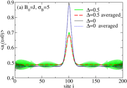
Figure 1: (Color online) Density profiles $\langle n_{i}(t=0)\rangle=M_{i}(t)+1/2$ in the initial state (time $t=0$), induced by (a) a Gaussian magnetic field Eq. (11) ($B_{0}=J,\sigma_{B}=5$); (b) a box-shaped magnetic field, Eq. (12) ($B_{0}=J$, $s_{B}=5$); and (c) application of $S^{+}_{L/2+1}$, all at half filling $n=0.5$. Thin solid lines in (a)-(c): $\Delta=0$; thick solid lines in (a): $\Delta=0.5$, thin and thick dashed lines in (a): averaged density $\langle\tilde{n}_{i}(t=0)\rangle$ for $\Delta=0$ and 0.5, respectively (see the text in Sec. IV for details on the averaging and Eq. (13)). Results at $\Delta=0$ are obtained with ED, all others with DMRG.

II.2 Methods

For the time-evolution of the noninteracting case ($\Delta=0$ in Eq. (2)), we use exact diagonalization which allows us to treat large systems. For all interacting cases, we employ the adaptive time-dependent DMRG methoddaley04 ; white04 ; vidal04 with a Krylov-space-based time-evolution schemepark86 ; hochbruck97 in the space of matrix product states.mcculloch07 The control parameters are the discarded weight $\delta\rho$ and the time-step $\delta t$. Our simulations are canonical ones as we work in subspaces with a fixed total $S^{z}$ or particle number, respectively. We have performed an extended error analysis by (i) comparing ED and tDMRG results in the noninteracting case and (ii) by performing several runs with different time-steps and discarded weights at representative parameters in the interacting case. Specifically, in case (i), we have analyzed the relative errors in the local magnetization

$$\delta M=\frac{1}{L}\sum_{i=1}^{L}|M_{i}^{DMRG}-M_{i}^{ED}|$$

and its variance (see below). It turns out that typically, a time step of $\delta t=0.125/J$ and a discarded weight of $\delta\rho=10^{-6}$ keeps the relative error $\delta M$ in $M$ below $10^{-4}$ for a chain of $L=200$ sites at half filling and for times $t\leq 100/J$.

III Ballistic vs diffusive transport

Within linear response theory, one often separates the dynamical conductivity $\sigma(\omega)$ into a delta-function $\delta(\omega)$ at zero frequency and a regular part at frequencies $\omega>0$,mahan ; zotos97

$$\sigma(\omega)=2\pi D\delta(\omega)+\sigma_{\mathrm{regular}}(\omega)\,.$$ (4)

These quantities derive from the Kubo formula that is based on evaluating current-current correlation functions.mahan We repeat that a finite Drude weight in a clean, one dimensional system at zero temperature defines an ideal conductor and thus ballistic behavior, while if $D=0$, one has an insulator.kohn64 ; scalapino93 The dependence of the Drude weight on the exchange anisotropy $\Delta$ in the case of the integrable $XXZ$ chain and at zero temperature is well-known:shastry90

$$D=\frac{\pi}{4}\frac{\sin\nu}{\nu(\pi-\nu)}\,,$$ (5)

where, in this equation, the anisotropy is parameterized through $\Delta=\cos(\nu)$. We thus have $D>0$ for $|\Delta|\leq 1$, featuring a discontinuous drop to zero at $\Delta=1$. Due to the excitation gap in the massive regime $\Delta>1$, we have a true insulator with $\sigma_{\mathrm{dc}}=0$ that can only transport magnetization once the gap has been exceeded by a sufficiently large external perturbation.

Similarly, the Drude weight vanishes in the massive phases of both the spin ladder and the frustrated chain, while in the massless regime of the latter model $D$ is finite at $T=0$.bonca94 ; furukawa08

Strictly speaking, on all systems with open boundary conditions, the Drude weight vanishes identically. Yet, it turns out that the corresponding weight is just shifted to small but finite frequencies,kuehner00 ; rigol08 and thus the system is expected to still exhibit ballistic and anomalous transport properties.

To justify and motivate our way of analyzing ballistic and diffusive transport, let us, for pedagogical reasons, consider a 1D system that obeys the diffusion equation:

$$\partial_{t}\rho(x,t)=\nabla\cdot(\mathcal{D}\nabla\rho(x,t))\,.$$ (6)

Here, $\rho(x,t)$ denotes, e.g., a particle density, and $\mathcal{D}$ the diffusion constant. The Green’s function associated with this equation is, in a $d$-dimensional setup, given by

$$G(x,\acute{x},t)=\frac{1}{(4\pi\mathcal{D}t)^{d/2}}\cdot e^{-\frac{(x-\acute{x})^{2}}{4\mathcal{D}t}}\,.$$ (7)

Therefore, we can calculate the expectation values

$$\langle x\rangle(t)=\acute{x}\ \mbox{and}\ \langle x^{2}\rangle=|\acute{x}|^{2}+2\,d\mathcal{D}t$$ (8)

and see that the variance $\sigma_{x}^{2}=\langle x^{2}\rangle-\acute{x}^{2}$ is linear in $t$ for normal diffusive transport. On the contrary, for ballistic dynamics, one expects the variance $\sigma_{x}^{2}$ to grow quadratically in time, as is well-known from elementary quantum mechanics for free particles.

Given a distribution of $M_{i}(t)=\langle n_{i}(t)\rangle-1/2$ at a time $t$, we find it most straightforward to compute the variance from the corresponding particle density distribution $\langle n_{i}(t)\rangle=M_{i}(t)+1/2$ as this is a positive quantity. We then compute the variance from

$$\sigma_{M}^{2}(t)=\frac{1}{(L/2)}\sum_{i=1}^{L}(i-\mu_{n})^{2}\cdot\langle n_{i}(t)\rangle\,.$$ (9)

where $\mu_{n}$ is the first moment of the normalized distribution $\langle n_{i}\rangle$. Note that we normalize $\langle n_{i}\rangle$ on the actual number of fermions rather than the system size.

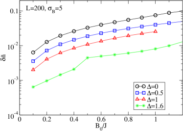
Figure 2: (Color online) Average deviation $\delta\tilde{n}$ from half filling [see Eq. (14)] in the initial state prepared by applying a Gaussian magnetic field [Eq. (11)] with $\sigma_{B}=5$ as a function of $B_{0}$ for $\Delta=0,0.5,1$ and $1.6$.

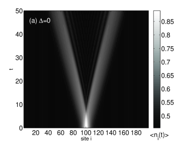
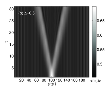
Figure 3: (a), (b) Time-evolution of the density (magnetization) profile $\langle n_{i}(t)\rangle=M_{i}(t)+1/2$ for a Gaussian initial state with $B_{0}=J$, $\sigma_{B}=5$ for (a): $\Delta=0$ (ED data) and (b): $\Delta=0.5$ (DMRG data, $L=200$ sites).

IV Preparation of initial states

We consider three different ways of preparing the initial state, which we now illustrate for the case of the $XXZ$ chain, Eq. (1), and at half filling $n=0.5$, i.e., at $S^{z}=0$. With the exception of Sec. V.2.2, our simulations are always performed in subspaces with these quantum numbers.

Technically, we add a term

$$H_{B}=-\sum_{i}B_{i}S_{i}^{z}$$ (10)

to the Hamiltonian. By choosing the $B_{i}$ appropriately, this realizes (i) a Gaussian magnetic field, (ii) a box-shape magnetic field, both applied during a ground-state DMRG run, and turned off at time $t=0$:

$$B_{i}(t=0) = B_{0}\,\mbox{exp}(-(i-i_{0})^{2}/2\sigma_{B}^{2})$$ (11)

$$B_{i}(t=0) = B_{0}\,\Theta\left(i-\frac{L-s_{B}}{2}\right)\Theta\left(i+\frac{L+s_{B}}{2}\right)\,.$$ (12)

$\Theta(i)$ is the Heaviside function. In Eq. (11), $\sigma_{B}$ is the variance of the external Gaussian field, $B_{0}$ its amplitude, and we set $i_{0}=L/2+0.5$, while in Eq. (12), $s_{B}$ denotes the width of a box in which a constant field $B_{0}$ is applied.

The third initial state (iii) is realized by finding the ground state of a system at filling $n=(L/2-1)/L$ and then applying a single spin flip $S^{+}_{i}$ on a site $i$. The time-evolution is then performed at half filling, as in cases (i) and (ii).

The typical shape of the induced density $\langle n_{i}(t=0)\rangle$, or equivalently, the magnetization profile is illustrated in Figs. 1(a)–(c) at $\Delta=0$ (all panels) and $\Delta=0.5$ (panel (a) only], for the three initial states (i)–(iii), respectively. Inherent to the fermionic nature of the model Eq. (2), we first observe Friedel oscillations with a $2k_{F}$ period, where $k_{F}=\pi/2$ is the Fermi momentum at half filling. Second, there are slower spatial oscillations, that are more evident in the case of $\Delta=0.5$ [Fig. 1(b)]. These oscillations’ characteristic wave-length depends, as we have checked, on $\sigma_{B}$ as well as the system size. As we shall see later, for the purpose of qualitatively analyzing the time-dependence of the variance, the presence of the long-ranged oscillations is irrelevant, as the dynamics stems from the cental peak dispersing, while away from the center, the oscillations contribute subdominantly to the time-dependence after turning off $H_{B}$. We will nevertheless sometimes find it illustrating and useful to work with a density

$$\langle\tilde{n}_{x}(t)\rangle=[\langle n_{2i-1}(t)\rangle+\langle n_{2i}(t)\rangle]/2\,$$ (13)

averaged over adjacent sites with $i=1,\dots,L/2$ and $x=2i-1/2$. To recover the variance of the non-averaged density, we multiply $\tilde{\sigma}_{M}^{2}$ by a factor of $2$. The averaged density $\langle\tilde{n}_{i}(t=0)\rangle$ is plotted with dashed lines in Fig. 1(a) for $\Delta=0$ and 0.5, and we see that this averaging results in quite smooth curves.

For $\langle\tilde{n}_{i}(t=0)\rangle$ and a Gaussian external $B_{i}$, we can now further address the question whether the induced density profile follows a Gaussian as well. We find that this is the case at small $\Delta$, in good approximation. In the massive phase $\Delta>1$, deviations of $\langle\tilde{n}_{i}(t=0)\rangle$ from a Gaussian profile are substantial. We will nevertheless refer to initial states prepared with Eq.(11) as Gaussian initial states throughout.

As we go from $\Delta=0$ into the massive regime $\Delta>1$, a gap opens, and qualitatively, despite the field $B_{i}$ being inhomogeneous, we expect the existence of the gap to affect the average deviation from half filling at a given set of $(B_{0},\sigma_{B})$. To illustrate this point, we display this average deviation $\delta\tilde{n}$, defined as

$$\delta\tilde{n}=\sqrt{\sum_{i}(\langle\tilde{n}_{i}\rangle-1/2)^{2}/N}\,,$$ (14)

in Fig. (2) ($\Delta=0,0.5,1,1.6$). For $\Delta=1.6$, we observe a steep increase in $\delta\tilde{n}$ at $B_{0}/J\approx 0.4$, and we will use $B_{0}/J>0.45$ for the time-evolution, as below this value, little dynamics in the time-evolution is seen. Note that Fig. 2 has a logarithmic scale on the $\delta\tilde{n}$ axis, and below $B_{0}/J\approx 0.4$, $\delta\tilde{n}\propto{\mbox{exp}}(c/B_{0})$ in the case of $\Delta=1.6$. We find $c=0.4J$ and this roughly coincides with twice the spin gap for this value of $\Delta$.cloizeaux66

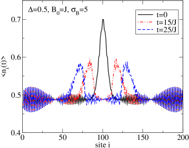
Figure 4: (Color online) Time-evolution of the density $\langle n_{i}(t)\rangle$ (or magnetization profile $M_{i}(t)=\langle n_{i}(t)\rangle-1/2$) for a Gaussian initial state with $B_{0}=J$, $\sigma_{B}=5$ at $\Delta=0.5$ (DMRG data, $L=200$ sites): Snap-shots from Fig. 3 at times $t\,J=0,15,25$.

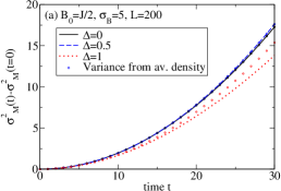
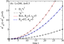
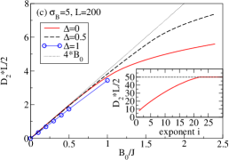
Figure 5: (Color online) (a) Time-dependence of the variance $\sigma_{M}^{2}(t)-\sigma_{M}^{2}(t=0)$ for $\Delta=0$ (solid lines) and $\Delta=0.5$ (dashed lines), both at $B_{0}=J/2$ and $\sigma_{B}=5$. Circles denote the variance $\tilde{\sigma}_{M}^{2}(t)-\tilde{\sigma}_{M}^{2}(t=0)$ of the averaged density $\langle\tilde{n}_{i}(t)\rangle$, Eq. (13). (b) Time-dependence of the variance $\sigma_{M}^{2}(t)-\sigma_{M}^{2}(t=0)$ for the evolution from a box-like initial state (solid line), after the application of $S^{+}_{L/2}$ (dot-dashed line), and from a Gaussian-state (dashed line) (all at $\Delta=0.5$). The squares denote the perfect fit of all sets to $\sigma_{M}^{2}(t)-\sigma_{M}^{2}(t=0)=D_{2}t^{2}$. (c) $B_{0}$-dependence of the coefficient $D_{2}$ of the time-dependent variance for $\Delta=0$ (solid lines), $\Delta=0.5$ (dashed lines), and $\Delta=1$ (circles) at a fixed $\sigma_{B}=5$ and $L=200$. The dotted lines display $D_{2}\,L/2=4B_{0}J$. Inset: $D_{2}(B_{0})$ in the limit of large $B_{0}=10^{i}J$ for $\Delta=0$. The thin dashed line is the result for the expansion from a Fock state of width $L/2$ with $\langle n_{i}\rangle=1$ at the center of the chain.

V The $XXZ$ chain

After detailing the way of preparing initial states, we now come to the analysis of $M_{i}(t)=\langle n_{i}(t)\rangle-1/2$, focusing on the variance $\sigma^{2}_{M}(t)$. In this section, we will first discuss $\sigma_{M}^{2}(t)$ in the massless regime in Sec. V.1, and show that we clearly see ballistic behavior with $\sigma_{M}^{2}(t)=\mbox{const}+D_{2}t^{2}$, independently of the initial state. We will then analyze the dependence of the coefficient $D_{2}$ on $B_{0}$, scanning the full range of perturbations from a linear one with $D_{2}\propto B_{0}$ to the largest perturbations possible. These regimes are distinct by a different finite-size scaling behavior, to be discussed below. As we illustrate in the case of a Gaussian magnetic field Eq. (11), ballistic dynamics is found for $\Delta\leq 1$. This holds independently of the actual choice of $(B_{0},\sigma_{B})$ and thus also far from equilibrium, except for the most extreme initial states considered here (see the discussion in Sec. V.1.2 below).

We then, in Sec. V.2, discuss the transition from ballistic to diffusive behavior which is expected to occur at $\Delta=1$. Our data are consistent with this picture, as we find strong evidence for diffusive transport for $\Delta\gtrsim 1.5$. We will present results for several $B_{0}$ at $\Delta=1.5$ to substantiate that the observation of diffusive transport is independent of the initial state.

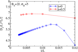
Figure 6: (Color online) Finite-size scaling of $D_{2}$ for $\Delta=0$ and 0.5 in the large $B_{0}$ regime ($B_{0}=2J$, $\sigma_{B}=5$).

V.1 $XXZ$ chain: Massless regime

V.1.1 Time-dependence of the variance

We now turn to the analysis of $M_{i}(t)=\langle n_{i}(t)\rangle-1/2$ in the massless regime. Figures 3(a) and (b) show $\langle n_{i}(t)\rangle=M_{i}(t)+1/2$ for $\Delta=0$ and $\Delta=0.5$, respectively. The initial density profile first melts and then, at times $t\,J\approx 5$, splits into two packets that travel into opposite directions.kollath05b Figure 4 shows snapshots of $\langle n_{i}(t)\rangle$ at times $t\,J=0,15,25$ for $\Delta=0.5$. It is noteworthy that, while substantial oscillations are present far away from the central peak, these oscillations are frozen in and do not contribute to the increase in $\sigma_{M}^{2}$ since, far away from the center of the chain, $H\approx H+H_{B}$.

The variance $\sigma_{M}^{2}(t)-\sigma^{2}_{M}(t=0)$, plotted vs. time, is displayed in Fig. 5(a), for $\Delta=0$ (solid line), $\Delta=0.5$ (dashed line), and $\Delta=1$ (dotted line) for the evolution from an initial state of the type (i), enforced by a Gaussian magnetic field with $B_{0}=J/2$ and $\sigma_{B}=5$. The circles represent the time-evolution of $\tilde{\sigma}^{2}_{M}(t)-\tilde{\sigma}^{2}_{M}(t=0)$ computed from the averaged density $\langle\tilde{n}(t)\rangle$ (see Sec. IV) for $\Delta=0,0.5,1$. For $\Delta=0$ and $0.5$, the averaged results very well coincide with $\sigma^{2}_{M}(t)$. For the purpose of characterizing ballistic or diffusive behavior, it therefore does not matter whether the pure fermionic density $\langle n_{i}(t)\rangle$ or the averaged quantity $\langle\tilde{n}_{i}(t)\rangle$ is used. In what follows, we will present results extracted from the former, unless stated otherwise. We mention, though, that the quantitative difference in the variance extracted from the averaged as compared to the bare density becomes more pronounced the larger $\Delta$ and the smaller $B_{0}$ is. This becomes evident in the case of $\Delta=1$, included in Fig. 5(a).

The key observation from Figs. 5(a) and (b) is the quadratic increase of the variance with time observed for $\Delta=0,0.5$ and 1, which confirms the expected ballistic behavior in the critical regime. For the isotropic chain ($\Delta=1$), we find that the best fit of a power-law to $\sigma^{2}_{M}(t)-\sigma^{2}_{M}(t=0)$ yields $\sigma^{2}_{M}(t)-\sigma^{2}_{M}(t=0)\propto t^{1.98}$, which is thus slightly below the behavior expected for ballistic transport. However, a deviation of just one percent from the expected exponent of 2 is very much within the accuracy of our numerical calculations.

Moreover, this behavior, as we show in Fig. 5(b) for the example of $\Delta=0.5$, is independent of the shape of the initial state: all three types of states studied here - Gaussian field, box shape, and application of $S_{i}^{+}$ - result in ballistic dynamics at half filling.

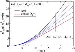
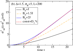
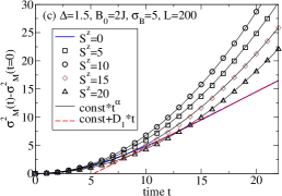
Figure 7: (Color online) (a) Transition from ballistic to diffusive transport: $\sigma^{2}_{M}(t)-\sigma^{2}_{M}(t=0)$ for $\Delta=1$ (thick solid line) $\Delta=1.2,1.3,1.4,1.5$ (thin solid lines). The parameters are $B_{0}=2J$, $\sigma_{B}=5$, $L=200$. The thick dashed line shows the asymptotic behavior for $\Delta=1.5$, i.e., $\sigma^{2}_{M}(t)=\mbox{const}+D_{1}t$. (b) Variance for $\Delta=1.5$ and several $B_{0}/J=1,1.5,2$ ($L=200$, $\sigma_{B}=5$). (c) Variance for $\Delta=1.5$ at $S^{z}=0,5,10,15,20$ (see the legend) and $B_{0}=2J$, $\sigma_{B}=5$: ballistic transport is restored away from half-filling.

V.1.2 From small to large perturbations

So far, we have worked at a fixed pair of $B_{0}$ and $\sigma_{B}$. We will now explore the dependence of the dynamics on how far the initial state is perturbed away from the actual ground state. This deviation is measured through the average deviation $\delta\tilde{n}$ from half filling (compare Fig. 2). For that purpose, we fix $\sigma_{B}=5$, and perform a set of simulations at different $B_{0}$, at $\Delta=0,0.5$ and 1. Independently of $B_{0}$, we always find a quadratic increase of $\sigma_{M}^{2}(t)$ with time, i.e., $\sigma_{M}^{2}(t)=\mbox{const}+D_{2}(B_{0})t^{2}$. As a main result, we therefore conclude that the qualitative behavior of the dynamics is independent of the external perturbation, it is always ballistic in the massless regime.

On a more quantitative level, it is instructive to plot $D_{2}$ vs $B_{0}$, shown in Fig. 5(c) for $\Delta=0$ and 0.5, as it allows us to distinguish two regimes: first, the linear regime, in which $D_{2}$ is linear in $B_{0}$ with $D_{2}\,L/2\not=f(L)$ at a fixed $B_{0}$. For $\Delta=0$ and 0.5, the linear regime extends up to $B_{0}/J\approx 0.5$. Second, at larger $B_{0}$ effects of both the band curvature and the finite band-width start to play a role, with significant finite-size effects, as illustrated in Fig. 6 for $B_{0}=2J$. In the case of $\Delta=0$ and $B_{0}=2J$, we are able to access system sizes of $L\approx 10^{5}$, and at large $L$, the scaling is of the form $D_{2}\,L/2\propto 1/L$, allowing for an extrapolation to $L\to\infty$. In the interacting case, the accessible system sizes are too small to establish such scaling and we thus have not attempted any extrapolation in the case of $\Delta=0.5$.

Let us next discuss the limiting cases of first, the linear regime, i.e., $D_{2}\propto B_{0}$, and second, the limit of $B_{0}\to\infty$. Starting with the former, the linear regime, $D_{2}\,L/2=\gamma B_{0}$, we find that the prefactor is $\gamma\approx 4J$ for values of $\Delta\lesssim 0.5$. At large $\Delta$, this reduces to $\gamma\approx 3.4J$ as the results for $\Delta=1$ displayed in Fig. 5(c) show (circles). The interpretation of $D_{2}$ being linear in $B_{0}$ for $\Delta\leq 1$ is based on the observation that the area $A_{\mathrm{peak}}(B_{0})$ under the initial Gaussian-like magnetization profile increases linearly in $B_{0}$, which we can strictly confirm in the $\Delta=0$ case and chains with up to $L=1000$ sites. This analysis requires an estimate of the background density, which can the best be done in the $\Delta=0$ case, but suffers from finite-size effects at a nonzero $\Delta$. In the $\Delta=0$ case, we find that $\gamma B_{0}/A_{\mathrm{peak}}(B_{0})=4J^{2}$ and for $\Delta=0.5$, $\gamma B_{0}/A_{\mathrm{peak}}(B_{0})\approx 1.7J^{2}$. We may therefore conclude that in the linear regime, $\gamma\,B_{0}=A_{\mathrm{peak}}(B_{0})\,v_{g}^{2}(\Delta)$, where $v_{g}(\Delta)$ is the group velocity (see, e.g., Ref. cabra-review, ):

$$v_{g}(\Delta)=\frac{\pi}{2}\frac{\sin(\nu)}{\nu}$$ (15)

with $\Delta=\cos(\nu)$. From our numerical data for $L=200$ sites and at $\Delta>0.5$, we obtain $D_{2}\,L/(2A_{\mathrm{peak}})>v_{g}^{2}(\Delta)$ due to finite-size effects, but qualitatively, $D_{2}\,L/(2A_{\mathrm{peak}})$ increases with $\Delta$ at a fixed $B_{0}$ in the linear regime as expected from Eq (15) for the behavior of the velocity $v_{g}^{2}$. At sufficiently large $B_{0}$, we expect the band-curvature to play a role as well which we are able to verify in the case of $\Delta=0$. $D_{2}\,L/(2A_{\mathrm{peak}})$ then decreases below $v_{g}^{2}(\Delta=0)$ as $B_{0}$ increases.

As for the limit of large $B_{0}\gg J$, note that since $M_{i}\leq 1/2$ and since we work at fixed half filling of the full system, the most extreme initial state that, on a fixed system size $L$, $B_{0}\to\infty$ drives the system into is a Fock state $|f\rangle$ with $\langle n_{i}(t=0)\rangle=1$ for $L/4<i<3L/4$ and zero otherwise. We thus follow the evolution from such a state as well as the evolution from states with very large $B_{0}\sim 10^{i}J$ ($i=1,\dots,30$). The inset in Fig. 5(c) shows that as $B_{0}$ increases, $D_{2}(B_{0})$ indeed approaches the value found for the limiting state $|f\rangle$ for $B_{0}>10^{22}J$ in the example of $\Delta=0$. In that limit, $D_{2}=1/2J^{2}$.

While for the parameters of the main panel of Fig. 5(c), i.e., $\Delta=0,0.5,1$ and $B_{0}/J\leq 2.4$, the variance always follows a power law with exponent two, curiously, this is not the case for the aforementioned Fock states encountered in the $B_{0}\to\infty$ limit and $\Delta=0.5,1$. There, we find exponents that are consistently below two for $\Delta>0$ and $L=40,80,200$. This behavior was also observed in Ref. gobert05, for the evolution from similar Fock states. A full analysis of the evolution from Fock states will be presented elsewhere.

We mention that the time-dependent evolution from Fock states or, more generally, the evolution of particles originally trapped in a confined region into an empty lattice, has been intensely studied with numerical methods in Refs. rigol04, ; rigol05b, ; rodriguez06, ; hm08a, , for the cases of hardcore bosons rigol04 ; rigol05b , soft-core bosons,rodriguez06 and the interacting two-component Fermi gas.hm08a These studies have a fundamental interest in out-of-equilibrium phenomena, with a perspective onto experiments with ultra-cold atoms in optical lattices. Among these we mention the experimental efforts directed at detecting Anderson localization in cold atom gases, precisely by utilizing such expansion set-ups.clement05 ; fort05

Finally, while all results discussed here were obtained from chains with $L=200$, we stress that we have carefully studied the finite-size scaling of $D_{2}$(see Figs. 5(c) and6). By plotting $D_{2}\,L/2$ in Fig. 5(c), we account for a trivial size-dependence, and curves obtained from different $L$ but the same $\Delta$ indeed collapse onto a single one in the linear regime. At larger $B_{0}$, $D_{2}$ tends to decrease with system size $L$ as less particles per $B_{0}$ can be accumulated in the initial Gaussian peak, due to $S_{i}^{z}\leq 1/2$ (see Fig. 6).

V.2 $XXZ$ chain: Massive phase

V.2.1 Transition from ballistic to diffusive behavior

Linear-response theory predicts a sharp transition from ballistic spin transport, characterized by a finite Drude weight $D$, to diffusive spin transport at $\Delta=1$.shastry90 We have carried out several simulations with different $\Delta=1,1.2,1.3,1.4,1.5$ at fixed parameters $B_{0}=2J$ and $\sigma_{B}=5$ to check whether an analysis of the variance captures this transition. As the data for $\sigma_{M}^{2}(t)$ displayed in Fig. 7(a) show, we clearly find a linear increase of $\sigma_{M}^{2}(t)$ at large times in the case of $\Delta=1.5$, which, in the sense of Sec. III, we interpret as evidence for diffusive transport. At smaller $1<\Delta\lesssim 1.4$, our data do not allow for this conclusion, yet at least we can state that the data for $\Delta=1.3$ and $1.4$ do not follow a power-law, indicative of non-ballistic transport. Also note that there is no contradiction with Eq. (5) as it is is well-known that finite-size effects in the vicinity of $\Delta=1$ are severe and come along with a logarithmically slow convergence with system size of quantities such as the Drude weight or the spin stiffness.laflorencie01 ; hm03 We suspect that larger system sizes, hence access to longer simulation times, are necessary to fully capture the sharp transition from ballistic to diffusive behavior at $\Delta=1$. We stress that with $B_{0}=2J$, we work with highly perturbed initial states, and thus the observation of diffusive transport for $\Delta\geq 1.5$ is a nontrivial one, going beyond the case studied in Ref. zotos97, . Our results for $\Delta\geq 1.5$ thus establish an example of diffusive dynamics with $\sigma_{M}^{2}(t)=\mbox{const}+D_{1}\,t$ in this model for the out-of-equilibrium situation. Note that a recent tDMRG work on transport in spin chains incorporating baths has reported similar results, derived from current and spin profiles in the steady state.prosen09

It is noteworthy that at short times, obviously, the dynamics is always ballistic, independently of $\Delta$, as can be seen in Fig. 7(a). Even the value of $\sigma_{M}^{2}(t)$ is roughly the same for all $\Delta$ at short times. In the long time limit, which is the relevant one to characterize the system as diffusive or ballistic, we find that $\sigma_{M}^{2}(t)$ systematically decreases with increasing $\Delta$. The reason is that, in the $\Delta/J\to\infty$ limit, no dynamics is possible at all.

We have further studied the dependence on $B_{0}$ at $\Delta=1.5$. In Sec. IV we hinted at the fact that at $\Delta>1$, a reasonably large $B_{0}$ is necessary to observe a significant change in the magnetization profile over the time scales simulated. We attribute this to the existence of a spin gap in the antiferromagnetic phase $\Delta>1$ and focus on $B_{0}\gtrsim J$. Our results of several runs at $\Delta=1.5$, scanning the $B_{0}$ dependence, are displayed in Fig. 7(b). We find that the variance increases with $B_{0}$, which we mainly attribute to more particles accumulated in the central peak. Furthermore, the figure suggests that the time-scale at which diffusive behavior sets in depends on $B_{0}$ such that for larger $B_{0}$, we are able to observe a linear increase of $\sigma_{M}^{2}(t)$ earlier in time.

V.2.2 Restoring ballistic transport

While so far we have restricted ourselves to the case of half filling, we now address the magnetization dynamics at incommensurate filling. The initial states are now created by applying the external fields in subspaces that already have a finite magnetization., i.e. $S^{z}\not=0$. Results for the variance at $\Delta=1.5$ are displayed in Fig. 7(c). The $z$-component of the total spin is $S^{z}=0,5,10,15,20$. We find that any nonzero $S^{z}$ is sufficient to render the dynamics ballistic again, on the time scales accessible to our simulations. According to our data, the variance follows $\sigma_{M}^{2}(t)-\sigma_{M}^{2}(t=0)\propto t^{\alpha}$, with $\alpha\approx 2.05\pm 0.02$. This observation is in agreement with the infinite-temperature behavior of the Drude weight,zotos97 ; hm05 which in the $XXZ$ chain is finite at any $\Delta$ away from half filling. Note that $\Delta>1$ and $S^{z}>0$ but below saturation is in the easy-plane phase of the $XXZ$ chain, with gapless excitations.review-frust Note that the prefactor in $\sigma_{M}^{2}(t)-\sigma_{M}^{2}(t=0)=D_{2}(S^{z})t^{\alpha}$ depends on $S^{z}$ in a non-monotonous way: it is the largest at around $S^{z}=10$ and then decreases as saturation is reached.

VI Nonintegrable models

We finally move on to the discussion of the dynamics in two nonintegrable models, the two-leg ladder and the frustrated chain, both limiting cases of Eq. (3). Numerical studies of the high-temperature limit, based on the Kubo formula, conclude that spin and thermal transport in the massive phases of these models (see Sec. II) are normal, with a vanishing Drude weight.hm03 ; hm04 ; hm07a ; zotos04 The conclusions on the massless phase of the frustrated chain are not unambiguous,hm03 ; jung06 ; hm07a ; jung07a and it has been pointed out that the energy-current operator, to first order in the next-nearest-neighbor interaction $\alpha J$, is conserved.jung06

Figure 8: Two-leg spin ladder with $J_{\parallel}=J_{\perp}$ [$\alpha=1$, $\delta=1$ in Eq. (3)]: Contour plot of $\langle n_{i}(t)\rangle=M_{i}(t)+1/2$. In the initial state, a Gaussian external field $B_{i}$ with $B_{0}=J$ and $\sigma_{B}=5$ is applied [see Eq. (11)]. DMRG data, $L=200$ sites.

One scenario is that the high-temperature Drude weight vanishes,hm03 ; hm04 while it is still possible to find anomalous transport properties in the low-temperature regime, e.g., in the form of a peculiar low-frequency behavior of $\sigma_{\mathrm{regular}}(\omega)$. Exact diagonalization results show that the Drude weight is finite at zero temperature in the massless phase of the frustrated chain.bonca94 ; furukawa08

We here use the approach outlined in the previous sections to show that the zero-temperature dynamics of two-leg ladders and frustrated chains with a spin gap is of diffusive nature. To this end, we prepare initial states with Gaussian magnetic fields Eq. (11). We emphasize that, in the case of the spin ladder, both sites on a rung experience the same field. In these two cases, and similar to the discussion of initial states for $\Delta>1$ in the $XXZ$ chain (compare Fig. 2 in Sec. IV), the amplitude of the Gaussian field, $B_{0}$, needs to be large enough to induce a substantial perturbation in the magnetization $M_{i}$ that will actually propagate through the system. We thus here probe the magnetization dynamics and transport at large external perturbations.

Starting with the example of a spin ladder with $J_{\perp}=J_{\parallel}$, we display the magnetization profile $M_{i}(t)=\langle n_{i}(t)\rangle-1/2$ in Fig. 8 as a contour plot. The time-dependence of the corresponding variance is shown in Fig. 9(a) [solid line, squares], and we find a linear increase in $\sigma_{M}^{2}(t)$ for times $t\gtrsim 17/J$, clearly establishing the notion of diffusive dynamics in the ladder system.

A more involved picture emerges in the case of the frustrated chain. For this model we present results for $\alpha=0.2$ (circles) and $\alpha=0.4$ (stars) in Fig. 9(b). While on the time scales simulated, the variance for the $\alpha=0.2$ curve perfectly follows the form $\sigma_{M}^{2}(t)=\mbox{const}+D_{2}t^{2}$ (a least-square fit to this function is displayed by a thin solid line), in the case of $\alpha=0.4$, we observe that the data do not follow a power law $\sigma_{M}^{2}(t)=\mbox{const}+D_{\alpha}t^{\alpha}$, which supports the notion of a time-dependent crossover from ballistic to diffusive dynamics. In fact, the numerical results yield a variance that clearly increases linearly in time for $t\gtrsim 30/J$. Note that the transition from the massless to the massive phase in this model is of the Beresinski-Kosterlitz-Thouless type,haldane82 ; okamoto92 ; white96 with an exponentially growing correlations lengths as the critical point $\alpha_{\mathrm{crit}}$ is approached from $\alpha>\alpha_{\mathrm{crit}}$. This renders it very difficult to see a sharp transition in the transport behavior using exact diagonalization or DMRG as $\alpha_{\mathrm{crit}}$ is crossed.

We mention, though, that for other values of $\alpha>\alpha_{\mathrm{crit}}\approx 0.241$ (results not shown here), on similar time-scales, no diffusive behavior is seen. Moreover, the time-scale at which diffusive dynamics emerges seems to strongly depend on $B_{0}$, i.e., on how far the initial state is perturbed over the actual ground state. The qualitative trend is that the larger $B_{0}$, the faster diffusive transport is established. Unfortunately, the larger $B_{0}$, the worse is the entanglement growth which renders tDMRG simulations more difficult (see, e.g., Ref. dechiara06, ).

Keeping in mind these remarks, we are in a position to conjecture that in general, in massive phases of one-dimensional spin models, spin transport is diffusive. Combined with the existing results for the high-temperature limit,hm03 ; hm07a ; zotos04 our work suggests that this observation applies independently of temperature.

Note that a recent exact diagonalization studysantos08 has promoted a different behavior, namely evidence for ballistic spin transport at zero temperature in the frustrated spin chain at $\alpha=1$. This conclusion is based on the presence of certain oscillations (dubbed a bouncing behavior)santos08 ; steinigeweg06 in $M_{i}(t)$ in the evolution from an initial state with all spins pointing up(down) in the left(right) part of an open system (compare Refs. antal99, ; gobert05, ). We believe that our analysis of the variance is more quantitative, which may imply that the oscillations in $M_{i}(t)$ reported on in Ref. santos08, are possibly of a different origin. A recent study of quantum quenches in the $XXZ$ chain proposes that oscillations seen in the order parameter are related to the quantum phase transition at $\Delta=1$ (Ref. barmettler09, , see also Ref. barthel08a, ).

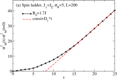
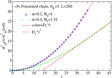
Figure 9: (Color online) Time dependence of the variance $\sigma^{2}_{M}(t)-\sigma^{2}_{M}(t=0)$. (a) Spin ladder, solid line with squares, compiled from the data of Fig. 8, $B_{0}=1.7J$. (b) Frustrated chain with $\alpha=0.2$ (circles, $B_{0}=J$) and a frustrated chain with $\alpha=0.4$ (stars, $B_{0}=1.5J$). In all cases, $\sigma_{B}=5$. The dashed lines in (a) and (b) are a fit of const$+D_{1}\,t$ to the variance of the spin-ladder and the frustrated chain with $\alpha=0.4$ at long times, while the thin, solid line in (b) is a least-square fit of $D_{2}\,t^{2}$ to the result for the frustrated chain with $\alpha=0.2$. DMRG data, $L=200$ sites.

VII Summary and Discussion

In this work we studied the nonequilibrium magnetization dynamics in one-dimensional spin models at zero temperature using the adaptive time-dependent DMRG method on system sizes as large as $L=200$ sites. We considered several models: the integrable spin-1/2 $XXZ$ chain, the frustrated chain, and the two-leg spin ladder. Based on the analysis of the time-dependence of the spatial variance of the magnetization during the time evolution starting from initial states with an inhomogeneous magnetization profile, we conclude that in the critical regime of the $XXZ$ chain, the magnetization dynamics is ballistic. In contrast to that, in the massive regime, our results indicate diffusive transport at half filling, while ballistic transport is restored away from half filling. A major aspect of our work is that we scanned the entire regime going from small to very strong perturbations over the ground state. This substantially extends previous studies of linear-response functions as we clearly enter into a regime with the system driven out of equilibrium. In the case of the massless regime of the $XXZ$ chain, ballistic transport is seen for substantially perturbed initial state, while for the most extreme initial states, i.e., pure Fock states, we still find a power-law for the time-dependence of the variance, but, on the times scales simulated, with an exponent below two.gobert05

As for the nonintegrable models, the frustrated chain and the ladder, the numerical data clearly support the notion of diffusive dynamics in the ladder system. In the case of the frustrated chain, our data are consistent with a transition from ballistic to diffusive behavior as the quantum critical point $\alpha_{\mathrm{crit}}\approx 0.241$ is crossed. In the limit of small perturbations, this result confirms with the general picture that massless phases support ballistic, and massive ones diffusive dynamics, at zero temperature and irrespective of integrability.scalapino92 Overall, a difference between the low- and high-temperature behavior is then evident: numerical results for the high-temperature limithm07a consistently support the notion of vanishing Drude weights in nonintegrable models, and thus normal transport behavior, irrespective of what the ground state phases are. Conversely, exact diagonalization studies find a finite Drude weight in the gapless phase of the frustrated spin-1/2 chain at zero temperature.bonca94 ; vieira01 ; furukawa08 In the low, or more extremely, zero temperature case, effective low-energy theories are expected to give a valid description, which typically predict diverging transport coefficients of clean spin systems (see, e.g., Ref. saito03, ). As for the heat transport measurements on spin chain and ladders experiments (see Refs. sologubenko07a, ; hess07a, for a survey), a dominant magnetic contribution is usually evident in the high-temperature regime, where the validity of effective low-energy theories for the description of transport is not obvious.

Finally, the approach of distinguishing ballistic from diffusive transport by analyzing the spatial variance of a density like quantity could be instrumental in characterizing ultracold atomic gases in optical lattices as well. There, one typically realizes the expansion of particles into an empty lattice, and experimentally it is possible to measure the expanding cloud’s radius. It would thus be very interesting to identify conditions for ballistic as compared to diffusive dynamics for model systems typically encountered in ultracold atomic gases such as the Bose-Hubbard model or a two-component Fermi gas in an optical lattice.

- (1) X. Zotos and P. Prelovšek, in: Strong Interactions in Low Dimensions, chapter 11, Physics and Chemistry of Materials with Low-Dimensional Structures, Kluwer Academic Publishers (Dordrecht), 2004.
- (2) F. Heidrich-Meisner, A. Honecker, and W. Brenig, Eur. J. Phys. Special Topics 151, 135 (2007).
- (3) W. Kohn, Phys. Rev. 133, A171 (1964).
- (4) D. J. Scalapino, S. R. White, and S. Zhang, Phys. Rev. Lett. 68, 2830 (1992).
- (5) X. Zotos, J. Phys. Soc. Jpn. Suppl. 74, 173 (2005).
- (6) B. N. Narozhny, A. J. Millis, and N. Andrei, Phys. Rev. B 58, R2921 (1998).
- (7) K. Fabricius and B. M. McCoy, Phys. Rev. B 57, 8340 (1998).
- (8) X. Zotos, Phys. Rev. Lett. 82, 1764 (1999).
- (9) J. V. Alvarez and C. Gros, Phys. Rev. Lett. 88, 077203 (2002).
- (10) F. Heidrich-Meisner, A. Honecker, D. C. Cabra, and W. Brenig, Phys. Rev. B 68, 134436 (2003).
- (11) D. A. Rabson, B. N. Narozhny, and A. J. Millis, Phys. Rev. B 69, 054403 (2004).
- (12) J. Benz, T. Fukui, A. Klümper, and C. Scheeren, J. Phys. Soc. Jpn. Suppl. 74, 181 (2005).
- (13) D. Heidarian and S. Sorella, Phys. Rev. B 75, 241104(R) (2007).
- (14) S. Fujimoto and N. Kawakami, Phys. Rev. Lett. 90, 197202 (2003).
- (15) H. Castella, X. Zotos, and P. Prelovšek, Phys. Rev. Lett. 74, 972 (1995).
- (16) A. Rosch and N. Andrei, Phys. Rev. Lett. 85, 1092 (2000).
- (17) X. Zotos and P. Prelovšek, Phys. Rev. B 53, 983 (1996).
- (18) S. Mukerjee, V. Oganesyan, and D. Huse, Phys. Rev. B 73, 035113 (2006).
- (19) S. Mukerjee and B. S. Shastry, Phys. Rev. B 77, 245131 (2008).
- (20) F. Heidrich-Meisner, A. Honecker, D. C. Cabra, and W. Brenig, Phys. Rev. B 66, 140406(R) (2002).
- (21) F. Heidrich-Meisner, A. Honecker, D. C. Cabra, and W. Brenig, Phys. Rev. Lett. 92, 069703 (2004).
- (22) X. Zotos, Phys. Rev. Lett. 92, 067202 (2004).
- (23) P. Jung, R. W. Helmes, and A. Rosch, Phys. Rev. Lett. 96, 067202 (2006).
- (24) P. Jung and A. Rosch, Phys. Rev. B 76, 245108 (2007).
- (25) P. Prelovšek, S. ElShawish, X. Zotos, and M.. Long, Phys. Rev. B 70, 205129 (2004).
- (26) G. Benenti, G. Casati, T. Prosen, and D. Rossini, Europhys. Lett. 85, 37001 (2009).
- (27) T. Antal, Z. Rácz, A. Rákos, and G. M. Schütz, Phys. Rev. E 59, 4912 (1999).
- (28) G. O. Berim, S. I. Berim, and G. G. Cabrera, Phys. Rev. B 66, 094401 (2002).
- (29) Y. Ogata, Phys. Rev. E 66, 066123 (2002).
- (30) V. Hunyadi, Z. Rácz, and L. Sasvari, Phys. Rev. E 69, 066103 (2004).
- (31) A. V. Sologubenko, T. Lorenz, H. R. Ott, and A. Freimuth, J. Low Temp. Phys. 147, 387 (2007).
- (32) C. Hess, Eur. Phys. J. Spec. Topics 151, 73 (2007).
- (33) A. V. Sologubenko, K. Gianno, H. R. Ott, U. Ammerahl, and A. Revcolevschi, Phys. Rev. Lett. 84, 2714 (2000).
- (34) C. Hess, C. Baumann, U. Ammerahl, B. Büchner, F. Heidrich-Meisner, W. Brenig, and A. Revcolevschi, Phys. Rev. B 64, 184305 (2001).
- (35) M. Otter, V. Krasnikov, D. Fishman, M. Pshenichnikov, R. Saint-Martin, A. Revcolevschi, and P. van Loodsrecht, J. Mag. Mag. Mat. 321, 796 (2009).
- (36) M. Takigawa, N. Motoyama, H. Eisaki, and S. Uchida, Phys. Rev. Lett. 76, 4612 (1996).
- (37) K.R. Thurber, A.W. Hunt, T. Imai, and F.C. Chou, Phys. Rev. Lett. 87, 247202 (2001).
- (38) J. Sirker, Phys. Rev. B 73, 224424 (2006).
- (39) F. L. Pratt, S. J. Blundell, T. Lancaster, C. Baines, and S. Takagi, Phys. Rev. Lett. 96, 247203 (2006).
- (40) C. Fort, L. Fallani, V. Guarrera, J. E. Lye, M. Modugno, D. S. Wiersma, and M. Inguscio, Phys. Rev. Lett. 95, 170410 (2005).
- (41) D. Clément, A. F. Varón, M. Hugbart, J. A. Retter, P. Bouyer, L. Sanchez-Palencia, D. M. Gangardt, G. V. Shlyapnikov, and A. Aspect, Phys. Rev. Lett. 95, 170409 (2005).
- (42) S. Trotzky, P. Cheinet, S. Fölling, M. Feld, U. Schnorrberger, A. M. Rey, A. Polkovnikov, E. A. Demler, M. D. Lukin, and I. Bloch, Science 319, 295 (2008).
- (43) T. Barthel, C. Kasztelan, I. P. McCulloch, and U. Schollwöck, Phys. Rev. A 79, 053627 (2009).
- (44) S. Grossjohann and W. Brenig, Phys. Rev. B 79, 094409 (2009).
- (45) S. R. White, Phys. Rev. Lett. 69, 2863 (1992).
- (46) S. R. White, Phys. Rev. B 48, 10345 (1993).
- (47) U. Schollwöck, Rev. Mod. Phys. 77, 259 (2005).
- (48) A. Daley, C. Kollath, U. Schollwöck, and G. Vidal, J. Stat. Mech.: Theory Exp. , P04005 (2004).
- (49) S. R. White and A. E. Feiguin, Phys. Rev. Lett. 93, 076401 (2004).
- (50) G. Vidal, Phys. Rev. Lett. 93, 040502 (2004).
- (51) K. Saito, Europhys. Lett. 61, 34 (2003).
- (52) R. Steinigeweg, J. Gemmer, and M. Michel, Europhys. Lett. 75, 406 (2006).
- (53) C. Mejia-Monasterio and H. Wichterich, Eur. Phys. J. Spec. Topics 151, 113 (2007).
- (54) M. Michel, O. Hess, H. Wichterich, and J. Gemmer, Phys. Rev. B 77, 104303 (2008).
- (55) T. Prosen and M. Znidaric, J. Stat. Mech: Theor. Exp. , P02035 (2009).
- (56) T. D. Kühner, S. R. White, and H. Monien, Phys. Rev. B 61, 12474 (2000).
- (57) D. Gobert, C. Kollath, U. Schollwöck, and G. Schütz, Phys. Rev. E 71, 036102 (2005).
- (58) B.S. Shastry and B. Sutherland, Phys. Rev. Lett. 65, 243 (1990).
- (59) X. Zotos, F. Naef, and P. Prelovšek, Phys. Rev. B 55, 11029 (1997).
- (60) F. Heidrich-Meisner, A. Honecker, and W. Brenig, Phys. Rev. B 71, 184415 (2005).
- (61) K. Louis and C. Gros, Phys. Rev. B 67, 224410 (2003).
- (62) K. Sakai and A. Klümper, J. Phys. Soc. Jpn. Suppl. 74, 196 (2005).
- (63) C. Kollath, U. Schollwöck, J. von Delft, and W. Zwerger, Phys. Rev. A 71, 053606 (2005).
- (64) P. Schmitteckert, Phys. Rev. B. 70, 121302(R) (2004).
- (65) G. D. Mahan, Many-Particle Physics, Plenum Press, New York, 1990.
- (66) H.-J. Mikeska and A. K. Kolezhuk, Lect. Notes Phys. 645, 1 (2004).
- (67) A. Klümper, Lect. Notes Phys. 645, 349 (2004).
- (68) E. Dagotto, Rep. Prog. Phys. 62, 1525 (1999).
- (69) E. Dagotto and T. M. Rice, Science 271, 618 (1996).
- (70) T. Park and J. Light, J. Chem. Phys 85, 5870 (1986).
- (71) M. Hochbruck and C. Lubich, SIAM J. Numer. Anal. 34, 1911 (1997).
- (72) I. P. McCulloch, J. Stat. Mech.: Theory Exp. , P10014 (2007).
- (73) D. J. Scalapino, S. R. White, and S. C. Zhang, Phys. Rev. B 47, 7995 (1993).
- (74) J. Bonča, J. P. Rodriguez, J. Ferrer, and K. S. Bedell, Phys. Rev. B 50, 3415 (1994).
- (75) S. Furukawa, M. Sato, Y. Saiga, and S. Onoda, J. Phys. Soc. Jpn. 77, 123712 (2008).
- (76) M. Rigol and B. S. Shastry, Phys. Rev. B 77, 161101(R) (2008).
- (77) J. des Cloizeaux and M. Gaudin, J. Math. Phys. 7, 1384 (1966).
- (78) D. C. Cabra and P. Pujol, Lect. Notes Phys. 645, 253 (2004).
- (79) M. Rigol and A. Muramatsu, Phys. Rev. Lett. 93, 230404 (2004).
- (80) M. Rigol and A. Muramatsu, Phys. Rev. Lett. 94, 240403 (2005).
- (81) K. Rodriguez, S. Manmana, M. Rigol, R. Noack, and A. Muramatsu, New J. Phys. 8, 169 (2006).
- (82) F. Heidrich-Meisner, M. Rigol, A. Muramatsu, A. E. Feiguin, and E. Dagotto, Phys. Rev. A 78, 013620 (2008).
- (83) N. Laflorencie, S. Capponi, and E. S. Sørensen, Eur. Phys. J B 24, 77 (2001).
- (84) F. D. M. Haldane, Phys. Rev. B 25, 4925 (1982).
- (85) K. Okamoto and N. Nomura, Phys. Lett. 169A, 433 (1992).
- (86) S. R. White and I. Affleck, Phys. Rev. B 54, 9862 (1996).
- (87) G. D. Chiara, S. Montangero, P. Calabrese, and R. Fazio, J. Stat. Mech.: Theory Exp. , P03001 (2006).
- (88) L. F. Santos, Phys. Rev. E 78, 031125 (2008).
- (89) P. Barmettler, M. Punk, V. Gritsev, E. Demler, and E. Altman, Phys. Rev. Lett. 102, 130603 (2009).
- (90) V. R. Vieira, N. Guihéry, J. P. Rodriguez, and P. D. Sacramento, Phys. Rev. B 63, 224417 (2001).
- (91) K. Saito, Phys. Rev. B 67, 064410 (2003).