The Connection between a Lyman Limit System, a very strong O VI Absorber, and Galaxies at $z\sim 0.203$

Abstract

With a column density $\log N($O VI$)=14.95\pm 0.05$, the O VI absorber at $z_{\rm abs}\simeq 0.2028$ observed toward the QSO PKS 0312–77 ($z_{\rm em}=0.223$) is the strongest yet detected at $z<0.5$. At nearly identical redshift ($z_{\rm abs}\simeq 0.2026$), we also identify a Lyman limit system (LLS, $\log N($H I$)=18.22\,^{+0.19}_{-0.25}$). Combining FUV and NUV spectra of PKS 0312–77 with optical observations of galaxies in the surrounding field ($15\arcmin\times 32\arcmin$), we present an analysis of these absorbers and their connection to galaxies. The observed O I/H I ratio and photoionization modelling of other low ions indicate the metallicity of the LLS is $[{\rm Z/H}]_{\rm LLS}\simeq-0.6$ and that the LLS is nearly 100% photoionized. In contrast, the O VI-bearing gas is collisionally ionized at $T\sim(3$–$10)\times 10^{5}$ K as derived from the high-ion ratios and profile broadenings. Our galaxy survey reveals 13 ($0.3\lesssim L/L_{*}\lesssim 1.6$) galaxies at $\rho<2h^{-1}_{70}$ Mpc and $|\delta v|\lesssim 1100$ ${\rm km\,s}^{-1}$ from the LLS. A probable origin for the LLS is debris from a galaxy merger, which led to a $0.7L_{*}$ galaxy ($[{\rm Z/H}]_{\rm gal}\simeq+0.15$) at $\rho\simeq 38h^{-1}_{70}$ kpc. Outflow from this galaxy may also be responsible for the supersolar ($[{\rm Z/H}]_{\rm abs}\simeq+0.15$), fully ionized absorber at $z_{\rm abs}\simeq 0.2018$ ($-190$ ${\rm km\,s}^{-1}$ from the LLS). The hot O VI absorber likely probes coronal gas about the $0.7L_{*}$ galaxy and/or ($\sim$0.1 keV) intragroup gas of a spiral-rich system. The association of other strong O VI absorbers with LLS suggests they trace galactic and not intergalactic structures.

1. Introduction

Connecting the QSO absorbers with their environments is crucial for using the absorbers to study the properties and evolution of galaxies, the intergalactic medium (IGM), and the galaxy-IGM interface. The taxonomy of QSO absorbers is usually made according to their H I column densities ($N($H I$)$): the Ly$\alpha$ forest (Rauch, 1998) with $\log N($H I$)<16$, the Lyman limit systems that are optically thick at the Lyman limit (LLS; Tytler, 1982) with $16\leq\log N($H I$)<20.3$, and the damped Ly$\alpha$ absorbers (DLAs; Wolfe et al., 2005) with $\log N($H I$)\geq 20.3$. Given their placement in the H I column density hierarchy, the LLS likely represent the interface between the tenuous, highly ionized Ly$\alpha$ forest and the dense, neutral DLAs.

Many observational studies have been undertaken to connect these absorbers to physical objects, such as galaxies, galaxy halos, intergalactic voids. At $z\lesssim 1$, analyses of the absorber-galaxy relationship show that QSO absorbers are not distributed randomly with respect to galaxies, even for absorbers with the lowest H I column densities detected so far (e.g., Lanzetta et al., 1995; Tripp et al., 1998; Impey et al., 1999; Chen et al., 2001; Bowen et al., 2002; Penton et al., 2002; Stocke et al., 2006; Wakker & Savage, 2008). Strong Mg II absorbers are found within the extended halos (impact parameter $\rho<100$ kpc) of individual galaxies (e.g., Bergeron & Boissé, 1991; Steidel, 1993), while the DLA are generally associated with the main bodies of galaxies (e.g., Chen & Lanzetta, 2003; Rao et al., 2003; Wolfe et al., 2005). Although strong Mg II absorbers are believed to be tracers of LLS, there is a large scatter between $W_{\lambda}($Mg II$)$ and $N($H I$)$, not allowing a direct connection between these two quantities (Churchill et al., 2005; Ménard & Chelouche, 2008), but see also Bouché (2008). Furthermore the origin, metallicity, and physical properties of the Mg II-bearing gas is largely unknown because of the limited information available (e.g., metallicity, ionization and physical conditions). This requires high spectral resolution UV space-based observations at $z\lesssim 1$ where several H I Lyman series lines and metal lines in various ionization stages combined with galaxy redshift surveys and imaging can be acquired.

Currently, there are only three reported LLS where detailed information about their metallicity, ionization, and galaxy environment is available. Those are at $z=0.08092$ toward PHL 1811 (Jenkins et al., 2003, 2005), $z=0.16710$ toward PKS 0405–123 (Chen & Prochaska, 2000; Prochaska et al., 2004, 2006; Williger et al., 2006), and $z=0.09847$ toward PKS 1302–102 (Cooksey et al., 2008). These studies suggest that LLS can be either metal-rich ($Z$$\sim$$0.5$–$1Z_{\odot}$) or metal poor ($Z\lesssim 0.02Z_{\odot}$) and are generally associated with the extended reaches ($\sim 30$–100 kpc) of individual galaxies. Combined with previous studies, these conclusions demonstrate that LLS are crucial for understanding the interaction between galaxies and their environments, an important ingredient in any cosmological simulations (e.g., Bertone et al., 2007; Oppenheimer & Davé, 2008a).

In this paper, we present another detailed study of the relationship between a LLS observed at $z=0.20258$ toward the QSO PKS 0312–77 ($z_{\rm em}=0.2230$) and galaxies. This QSO was originally observed in the UV using the high-resolution mode of Space Telescope Imaging Spectrograph (E140M, E230M) onboard of the Hubble Space Telescope (HST) to study the Magellanic Bridge (see Lehner et al., 2008), a region of gas linking the Small and Large Magellanic Clouds (SMC, LMC). The STIS spectrum revealed very strong Ly $\alpha$ and Ly $\beta$ absorption lines, suggesting the presence of a LLS. This was subsequently confirmed by Far Ultraviolet Spectroscopic Explorer (FUSE) observations where the expected flux decrement at the Lyman limit at $z\approx 0.203$ is detected. We show that the H I column density (that often lacks in low resolution surveys of Lyman thick absorbers) can be determined owing to the high spectral resolution of these spectrographs. Determining $N($H I$)$ is crucial as it allows us to determine the metallicity and ionization conditions of the LLS.

At a similar redshift, this sightline also reveals the strongest O VI absorber discovered to date, with $\log N($O VI$)=14.95\pm 0.05$ (see §3.3). Strong O VI absorbers are rare and are unlikely to be related to the warm-hot intergalactic medium (WHIM, Cen & Ostriker, 1999; Davé et al., 1999), where a large fraction of the baryons could reside at $z<0.5$. Oppenheimer & Davé (2008b) argued that strong O VI collisionally ionized absorbers are related to the recycling of gas between the IGM and galaxies. Their conclusions are based on Gadget-2 cosmological simulations that included a variety of wind models and input physics variations. The strong O VI absorbers may therefore be higher redshift counterparts of O VI absorption that probes the extended halos of galaxies, such as in our Galaxy (Savage et al., 2003) and the LMC (Howk et al., 2002b; Lehner & Howk, 2007). The strong O VI  absorbers may also probe cooling gas from intragroup medium revealed by soft X-rays observations or even possibly relatively cool (0.1–0.3 keV) intragroup gas (Mulchaey et al., 1996). Recent surveys at low $z$ show indeed that, as for the H I and low-ion absorbers, O VI absorbers are not usually found in intergalactic voids but within $\lesssim 600$–800 kpc of galaxies (Stocke et al., 2006; Wakker & Savage, 2008). These works, however did not address explicitly the origin(s) of very strong ($\log N>14.5$) O VI absorbers. Hence this sightline provides the unique opportunity to study simultaneously the interaction of galaxies with their surroundings using very different tracers of gas-phases and energies and to test recent cosmological simulations.

The organization of this paper is as follows. After describing the observations and data reduction of the PKS 0312–77 UV spectrum in §2, we present our analysis to estimate the redshifts, equivalent-widths ($W_{\lambda}$), and column densities ($N$), of the absorbers in §3. In §4 we determine the physical properties and abundances of the metal-line absorbers observed at $z\approx 0.203$, while in §5 we present our galaxies survey and discuss the relationship between the absorbers and galaxies. In §6 we briefly discuss that current observations of the galaxy-IGM absorbers show compelling evidence that the LLS and strong O VI absorbers trace the galaxy-intergalactic interface, i.e. the galactic environments on physical scale of tens to hundreds of kpc around galaxies. A summary of the main results is presented in §7. For the reader’s information, all distances in this paper are physical separations derived from the angular diameter spaces, assuming a $\Lambda$CDM cosmology with $\Omega_{m}=0.3$, $\Lambda=0.7$, and $H_{0}=70$ ${\rm km\,s}^{-1}$ Mpc^-1 (we use the notation $h_{70}=H_{0}/70\,{\rm km\,s^{-1}\,Mpc^{-1}}$).

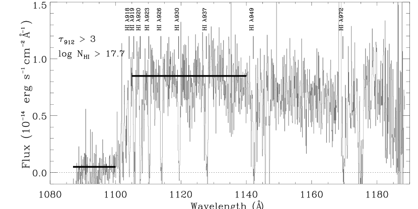
Figure 1.— Lyman limit at $z=0.20258$ observed in the FUSE spectrum. The H I lines used in our profile fitting are indicated (the Ly$\gamma$ line is shown but not used because it is contaminated by an airglow emission line). Other absorption lines are either interstellar or other intervening IGM features. From the flux decrement, we can place a limit on the H I optical depth at the Lyman limit and hence on the H I column density (the flux levels to estimate the the optical depth at the Lyman limit are shown with horizontal thick solid lines). For display purposes, the data are binned to the FUSE resolution, i.e. 1 pixel is about 20 ${\rm km\,s}^{-1}$.

2. UV Spectroscopic Observations

In this work, we present UV observations of the $z\approx 0.203$ absorber detected in the spectra of the QSO PKS 0312–77. The far to near UV spectra of PKS 0312–77 were obtained with FUSE (1080–1190 Å, $R\approx 15,000$; program F108 and E848 – PI: Lehner and Sembach, respectively) and HST/STIS 140M (1170–1730 Å, $R\approx 44,000$) and E230M (2130–2980 Å, $R\approx 30,000$) (program 8651, PI: Kobulnicky). The total exposure times are 37.9 ks for the E140M grating, 6.1 ks for the E230M grating, and 55.5 ks for FUSE (for LiF 2A+LiF 1B segments). The entrance slit for STIS was set to $0\farcs 2\times 0\farcs 2$, while the $30\arcsec\times 30\arcsec$ square (LWRS) aperture was used for FUSE. Typical signal-to-noise (S/N) ratios are about 4–7 per resolution elements (about 7 ${\rm km\,s}^{-1}$ for E140M, 10 ${\rm km\,s}^{-1}$ for E230M, and 20 ${\rm km\,s}^{-1}$ for FUSE). Unfortunately, only about 20% of the requested time was obtained for the FUSE program F018 before the failure of the telescope. Yet as illustrated in Figs. 1 and 2 the FUSE data are particularly useful for identifying the flux decrement at the Lyman limit at $z=0.20258$ and the Lyman series lines, which allow a secure determination of the H I column in the $z\approx 0.203$ absorber (see below). The full STIS spectrum is shown in T. Miwava et al. (in prep.), but see Fig. 3 for the normalized profiles of selected species (see below). In the E140M spectrum, the S/N ratio can increase up to about 15 in the QSO emission lines (e.g., near the N V doublet at $z=0.20258$, S/N $\simeq$15). On the other hand, at $\lambda\lesssim 1185$ Å and $\lambda\gtrsim 1650$ Å, the S/N ratio in the E140M spectrum is very low (S/N $\lesssim 2$–3).

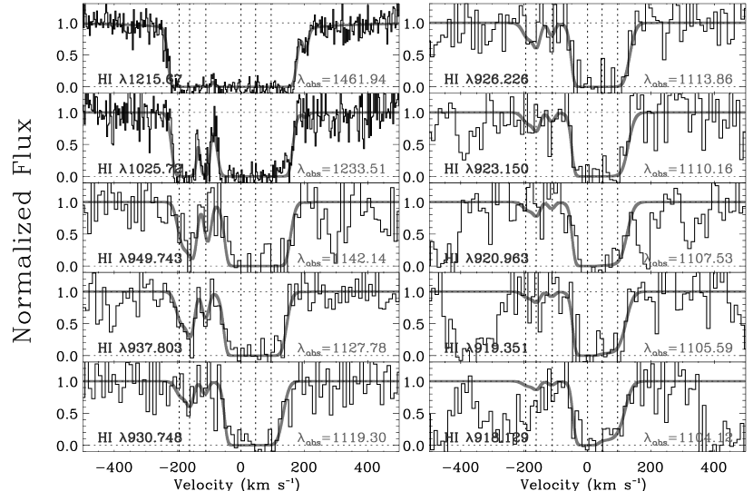
Figure 2.— Normalized H I profiles relative to $z=0.20258$. The solid line shows our fit to the data. The vertical dotted lines show the velocity centroids of the various components that were used as input in the profile fitting (see Table 1).

The STIS data were reduced using the STIS ID Team version of calstis at the Goddard Space Flight Center. The procedure for reduction of the STIS E140M data is fully described in Tripp et al. (2008) and includes the two-dimensional echelle scattered light correction (Valenti et al., 2002) and the algorithm for automatic repair of hot pixels (Lindler, 2003). The FUSE data were calibrated using the calfuse version (v3.2, Dixon et al., 2007). In order to achieve the optimum signal-to-noise, LiF 2A and LiF 1B segments were coadded. We note that the continuum of the QSO is not well behaved on large wavelength scales, but its “bumpiness” is unlikely due to the “worm” effect (see Dixon et al., 2007) since the fluxes in LiF 1B and LiF 2A match each other quite well (a similar behavior is also at longer wavelengths in the STIS bandpass). The fluxes in the individual exposures are too low to resolve the interstellar lines, so the separate exposures were simply co-added. Inspection of the resulting spectrum and comparison with common interstellar lines in the STIS spectrum indicates a posteriori no large shifts were necessary. The oversampled FUSE spectra were binned to a bin size of 0.04 Å, providing about two samples per $\sim$20 ${\rm km\,s}^{-1}$ resolution element.

The profiles were normalized using Legendre polynomials within $\pm$500–2000 ${\rm km\,s}^{-1}$ of each absorption line of interest. The continua are simple enough that the orders of the polynomial used to fit them were low ($\leq 4$).

3. Absorbers Analysis

To derive the column densities and measure the redshifts, we used the atomic parameters compiled by Morton (2003).

3.1. Kinematics Overview

The normalized profiles of the H I and other species are shown in Figs. 2 and 3 against the restframe velocity at $z=0.20258$ (see below for this choice). The profiles are complex with several components. From the H I profiles (Ly$\beta$ and Ly$\delta$; Ly$\gamma$ is very noisy in STIS and is not used here, while in FUSE Ly$\gamma$ is contaminated, see Fig. 1), we can decipher at least 5 blended components at about $-200$, $-160$, $-110$, $+50$, and $+205$ ${\rm km\,s}^{-1}$. In the $+50$ ${\rm km\,s}^{-1}$ component, there is some evidence for at least another component near $0$ ${\rm km\,s}^{-1}$, but the absorption is too strong to be conclusive.

The combination of weak and strong metal lines allows us to better explore the component structures. The Fe II $\lambda$1144 and Fe III $\lambda$1122 profiles show that the main absorption occurs at 0 ${\rm km\,s}^{-1}$. This component is also observed in the profiles of C II, N II, Si II, S II, and O I. The latter is quite weak (see §3.3), but is nevertheless detected at 3$\sigma$. As O I is one of the best tracers of neutral hydrogen, the positive detection of O I $\lambda$1302 at $z=0.20258$ (in agreement with the strong absorption in other species) sets the zero velocity point of the LLS. Examining the stronger lines (Si II, Si III, C II, N II) shows other components at $-195$, $-162$, $-111$, $+46$, and $+95$ ${\rm km\,s}^{-1}$. Except for the latter, these components are also discerned in the H I profiles, implying that the H I- and metal-line components follow each other extremely well.

3.2. H I Column Densities

The H I Lyman series lines are detected from Ly$\alpha$ down to the Lyman Limit (see Figs. 1 and 2). From the flux decrement observed at the Lyman limit, we find the optical depth $\tau_{LL}>3$ and via $\tau_{LL}=\sigma_{LL}N($H I$)$ (where $\sigma_{LL}=6.3\times 10^{-18}$ cm^-2 is the photoionization cross-section for hydrogen; Spitzer 1978 and Osterbrock 1989), we can place a firm lower limit on the H I column density (Fig. 1): $\log N($H I$)>17.7$. In Fig. 1, the thick solid shows the adopted flux levels blueward and redward of the break. As the continuum is not a straight line, we note that a change in the flux level redward of the break of $\pm 0.1\times 10^{-14}$ erg s^-1 cm^-2 Å^-1 would change the limit on the column density by only about $\pm 0.1$ dex. We estimate the flux blueward of the break to be $<0.04\times 10^{-14}$ erg s^-1 cm^-2 Å^-1.

The total equivalent width of Ly $\alpha$ is $1768\pm 35$ mÅ, which would imply that $\log N($H I$)\approx 18.8$ if it is on the square root part of the curve of growth. It is an upper limit because there is no evidence of damping wings in the Ly$\alpha$ profile (see also below). However, as we argue above, the Lyman limit system is confined to $>-80$ ${\rm km\,s}^{-1}$. Based on the weaker Lyman series lines (see Table 2), we integrate the Ly $\alpha$ absorption from $-80$ to $+140$ ${\rm km\,s}^{-1}$to find $W_{\lambda}\simeq 950$ mÅ, implying $\log N($H I$)<18.3$.

From these limits, the H I column density is $17.7<\log N($H I$)<18.3$. In order to refine the H I column density, we also fitted the absorption Lyman series lines with the Voigt component software of Fitzpatrick & Spitzer (1997). In the FUSE band, we assume a Gaussian instrumental spread function with a ${\rm FWHM_{inst}}=20$ ${\rm km\,s}^{-1}$, while in the STIS band, the STIS instrumental spread function was adopted (Proffitt et al., 2002). Note that our final fit does not use the Ly$\gamma$ line, but including this line would not have changed our results because it is so noisy (see Fig. 23 in Thom & Chen, 2008). For our adopted fit, we use the velocity-centroids of the components to those derived from the low ions as initial conditions (see §3.1 and column 2 in Table 1) but those are allowed to vary during the fitting procedure. The Doppler parameter $b$ and column density $N$ in each component are also allowed to vary freely. The results are summarized in Table 1 and the fits are shown in Fig. 2. The reduced-$\chi^{2}$ for the resulting fit is 1.23. For the Lyman limit system at $z\equiv 0.20258$, we find $\log N($H I$)=18.15\pm 0.25$, in agreement with the upper and lower limits derived above. The velocities of the H I derived from the fit are also in good agreement within $1\sigma$ from the velocities derived from the low ions (see columns 2 and 3 in Table 1).

Table 1Kinematics and Results from the H I Profiles Fit

$z$	$v$	$v_{\rm fit}$	$b$	$\log N$
	(${\rm km\,s}^{-1}$)	(${\rm km\,s}^{-1}$)	(${\rm km\,s}^{-1}$)
(1)	(2)	(3)	(4)	(5)
0.201798	$-195$	$-187\pm 11$	$21\pm 6$	$15.15\pm 0.33$
0.201930	$-162$	$-160\pm 7$	$12\pm 8$	$15.20\pm 0.31$
0.202135	$-111$	$-113\pm 1$	$11\pm 2$	$14.87\pm 0.16$
0.202580	$0$	$-1\pm 10$	$20\pm 8$	$18.15\pm 0.25$
0.202765	$+46$	$26\pm 11$	$43\pm 10$	$16.87\pm 0.56$
0.202961	$+95$	$85\pm 13$	$34\pm 5$	$16.62\pm 0.33$
0.203398	$+204$	$203\pm 3$	$10:$	$12.87\pm 0.16$

Note. — Column (1): Redshifts determined from the low metal ions.

Column (2): Velocities of the components determined from the low metal ions; $z=0.202580$ sets the zero-velocity.

Column (3): Velocities determined from the fit to H I line profiles.

Column (4): Doppler parameter determined from the fit to H I line profiles. A colon indicates that the value is uncertain (i.e. the error is of the order of the estimated value).

Column (5): Logarithmic of the column density (in cm^-2) determined from the fit to H I line profiles.

As the kinematics are complex and in particular the blending of the LLS with other H I absorbers at higher absolute velocities could hide the presence of damping wings, we also tested the robusteness of the fit by forcing the value of $N($H I$)$ at $z=0.20258$ to be 18.5 dex and letting the $b$ in this component and $b,N$ in the other components to vary freely. For this value, the damping wings start to appear at positive velocities, confirming that the H I column cannot be much greater than $10^{18.4}$ cm^-2.

As the FUSE instrumental resolution remains somewhat uncertain, we also investigated the results from the profile fitting using a Gaussian instrumental spread function with ${\rm FWHM_{inst}}=15$ and 25 ${\rm km\,s}^{-1}$, i.e. allowing for an error $\pm 5$ ${\rm km\,s}^{-1}$ in FWHM_inst. For all the components with $v\geq-120$ ${\rm km\,s}^{-1}$, an excellent agreement was found for $v,b,N$. Only in the components at $-195$ and $-162$ ${\rm km\,s}^{-1}$, we noticed a change in the column density with the most negative component being the strongest when ${\rm FWHM_{inst}}=25$ ${\rm km\,s}^{-1}$. However, the total column density in these two components was conserved. In view of the uncertainty, in the remaining of the text, we will only consider the total column density, $\log N($H I$)=15.49\pm 0.24$, of these components that we define as the absorber at $z\approx 0.2018$.

Finally we also also used a curve-of-growth (COG) method to test our results for the LLS and the absorber at $z\approx 0.2018$. As these H I absorbers are strong, using different analysis methods to determine $N($H I$)$ is valuable since comparisons of the results provide insights about systematic error measurements. The COG method used the minimization and $\chi^{2}$ error derivation approach outlined by Savage et al. (1990). The program solves for $\log N$ and $b$ independently in estimating the errors. In Table 2, we summarize our equivalent widths for these two absorbers. As the various components are strongly blended together, for the LLS, we did not use Ly$\alpha$. For the absorbers at $z=0.201798$ and $0.201930$, we combined these two absorbers (defined as the absorber at $z\approx 0.2018$). The results of the COG are for the LLS, $\log N($H I$)=18.28\,^{+0.02}_{-0.33}$ ($b=35\pm 2$ ${\rm km\,s}^{-1}$), and for the absorber at $z\approx 0.2018$, $\log N($H I$)=15.59\pm 0.16$ ($b=20\pm 1$ ${\rm km\,s}^{-1}$). These values are quite consistent with those obtained from the profile fit. For our adopted H I column densities, we take the mean between these two methods: $\log N($H I$)=18.22\,^{+0.19}_{-0.25}$ for the LLS and $\log N($H I$)=15.55\,^{+0.19}_{-0.24}$ for the absorber at $z\approx 0.2018$.

Table 2Equivalent Widths of the H I transitions used in the COG

$\lambda_{\rm rest}$	$\log(f\lambda)$	$W_{\rm rest}$
	(${\rm km\,s}^{-1}$)	(mÅ)
$z=0.20258$ – $[-80,+140]^{a}$ ${\rm km\,s}^{-1}$
1025.7222	1.909	$740\pm 37$
949.7430	1.122	$605\pm 69$
937.8034	0.864	$570\pm 61$
930.7482	0.476	$550\pm 56$
926.2256	0.470	$536\pm 56$
923.1503	0.311	$515\pm 59$
920.9630	0.170	$531\pm 62$
919.3513	0.043	$506\pm 61$
918.1293	$-0.072$	$467\pm 70$
$z\approx 0.2018$ – $[-235,-140]^{a}$ ${\rm km\,s}^{-1}$
1215.6700	2.704	$381\pm 19$
1025.7222	1.909	$266\pm 19$
949.7430	1.122	$137\pm 39$
937.8034	0.864	$140\pm 30$
930.7482	0.476	$54\pm 32$

Note. — $a:$ Velocity interval over which the equivalent widths were estimated. These intervals were defined using the uncontaminated weak H I transitions.

Previous surveys of the low redshift IGM have considered this line of sight and this absorber, although none has considered the key information from the FUSE observations. Thom & Chen (2008) fitted the H I column densities but only using Ly $\alpha$, Ly $\beta$, and Ly $\gamma$, resulting in a more uncertain fit (note that there is a velocity shift between our results and theirs because they adopted for the zero velocity point from the centroids of the O VI), but in overall agreement with our results for the LLS ($\log N($H I$)\sim 18.4$). Danforth & Shull (2008) attempted to use the COG method with Ly $\alpha$ and Ly $\beta$ equivalent widths and found $\log N($H I$)=15.14\,^{+0.21}_{-0.12}$ for the LLS, in contradiction with our results and the lower limit derived from the strong break at the Lyman limit. Finally, Tripp et al. (2008) only estimated a lower limit on the column density of the LLS that is not really constraining ($\log N($H I$)>14.72$). For the absorber at $z\approx 0.2028$, $N($H I$)$ values derived by these groups are systematically smaller by about 0.5 dex than our adopted value although our results overlap within about 1$\sigma$. The main difference is again that these groups did not use the weaker H I lines available in FUSE. We note that the apparent optical depth method (see §3.3) on the weaker $>3\sigma$ line (H I $\lambda$937) yields $\log N_{a}=15.43^{+0.13}_{-0.18}$, in agreement within 1$\sigma$ with our adopted value.

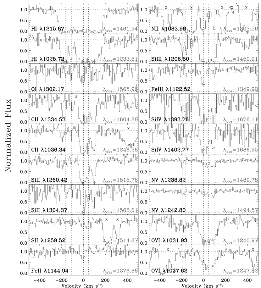
Figure 3.— Normalized profiles relative to $z=0.20258$ (ordered approximately by ionization potential). The vertical dotted lines show the velocity centroids of the various components. The absorber at $z\approx 0.2018$ is between $-220$ and $-150$ ${\rm km\,s}^{-1}$ in this representation, while the main absorption of LLS is between $-40$ and $+30$ ${\rm km\,s}^{-1}$, but with additional components up to $+130$ ${\rm km\,s}^{-1}$. The “x” shows part of the spectrum that is contaminated by other absorbing features.

3.3. Metal Lines

To estimate the column densities and the Doppler parameters of the atomic and ionic metal lines, we used the apparent optical depth (AOD, see Savage & Sembach, 1991). In this method, the absorption profiles are converted into apparent optical depth (AOD) per unit velocity, $\tau_{a}(v)=\ln[I_{\rm c}/I_{\rm obs}(v)]$, where $I_{\rm obs}$, $I_{\rm c}$ are the intensity with and without the absorption, respectively. The AOD, $\tau_{a}(v)$, is related to the apparent column density per unit velocity, $N_{a}(v)$, through the relation $N_{a}(v)=3.768\times 10^{14}\tau_{a}(v)/(f\lambda(\mbox{\AA})$) ${\rm cm}^{-2}\,({\rm km\,s^{-1}})^{-1}$. The total column density is obtained by integrating the profile, $N=\int_{v_{1}}^{v_{2}}N_{a}(v)dv$. For species that are not detected, we quote a 3$\sigma$ limit following the method described in Lehner et al. (2008).

Integration ranges for the equivalent widths and apparent column densities are listed in column 2 of Tables 3 and 4. Table 3 summarizes the total column densities and equivalent widths of both absorbers at $z=0.201798$ ($-195$ ${\rm km\,s}^{-1}$) and 0.201930 ($-162$ ${\rm km\,s}^{-1}$). We use this approach because, except for Si III, the spectra are too noisy to reveal both absorbers. Table 4 summarizes the results for the absorber directly associated to the LLS ($[v_{1},v_{2}]=[-40,+30]$ ${\rm km\,s}^{-1}$) or the absorbers associated to the LLS plus the absorption at higher positive velocities ($[v_{1},v_{2}]\approx[-50,+130]$ ${\rm km\,s}^{-1}$). The reason for the latter interval is because O VI and N V cannot be separated into different components, and strong saturated lines (e.g. Si III) do not show any structures in their profiles. As weaker transitions are only observed in the $[-30,+30]$ ${\rm km\,s}^{-1}$ interval, the column density in the LLS (0 ${\rm km\,s}^{-1}$) component dominates the total column density over $[-50,+130]$ ${\rm km\,s}^{-1}$ for the neutral, singly and doubly ionized species.

Table 3Measurements of the Metals at $z\approx 0.2018$ ($v\approx-190$ ${\rm km\,s}^{-1}$)

Species	$[v_{1},v_{2}]$	$W_{\rm rest}$	$\log N$
	(${\rm km\,s}^{-1}$)	(mÅ)
C II $\lambda$1334	$[-220,-165]$	$46\pm 23$	$13.7\,^{+0.1}_{-0.2}$
C II $\lambda$1036	$[-220,-165]$	$41\pm 9$	$13.68\pm 0.10$
C III $\lambda$977	$[-220,-150]$	$148\pm 42$	$>13.45$
N V $\lambda$1238	$[-210,-150]$	$29\pm 6$	$13.21\pm 0.08$
N V $\lambda$1242	$[-210,-150]$	$18\pm 5$	$13.27\,^{+0.11}_{-0.15}$
O VI $\lambda$1031	$[-210,-150]$	$59\pm 11$	$13.81\pm 0.09$
O VI $\lambda$1037	$[-210,-150]$	$27\pm 11$	$13.7\,^{+0.1}_{-0.2}$
Si II $\lambda$1260	$[-230,-170]$	$58\pm 12$	$12.61\pm 0.10$
Si II $\lambda$1193	$[-220,-160]$	$25\pm 10$	$12.6\pm 0.2$
Si III $\lambda$1206	$[-220,-145]$	$48\pm 13$	$>13.00$
Si IV $\lambda$1393	$[-225,-145]$	$178\pm 50$	$13.56\,^{+0.19}_{-0.34}$
Si IV $\lambda$1402	$[-225,-145]$	$105\pm 35$	$13.54\,^{+0.13}_{-0.20}$
Al III $\lambda$1854	$[-220,-150]$	$<189$	$<13.05$

Note. — Column density measurements were realized using the apparent optical depth by integrating the profiles over the velocity interval $[v_{1},v_{2}]$ (velocities are relative to $z=0.202580$). The column density of a feature detected in the 2–3$\sigma$ range is given only with one relevant digit. “$<$” indicates a 3$\sigma$ upper limit that was estimated over the velocity range observed in the absorption of other species. “$>$” indicates a lower limit.

Table 4Measurements of the Metals near $z\approx 0.2026$

Species	$[v_{1},v_{2}]$	$W_{\rm rest}$	$\log N$
	(${\rm km\,s}^{-1}$)	(mÅ)
C II $\lambda$1036	$[-40,+30]$	$229\pm 20$	$>14.31$
C II* $\lambda$1037	$[-40,+30]$	$<36$	$<13.51$
N I $\lambda$1199	$[-40,+30]$	$<39$	$<13.36$
N II $\lambda$1083	$[-40,+30]$	$193\pm 12$	$>14.26$
O I $\lambda$1302	$[-40,+30]$	$70\pm 23$	$14.17\,^{+0.14}_{-0.22}$
Si II $\lambda$1304	$[-40,+30]$	$182\pm 46$	$>14.12$
Al III $\lambda$1854	$[-40,+30]$	$<31$	$<13.15$
S II $\lambda$1259	$[-40,+30]^{a}$	$41\pm 11$	$\cdots$
S II $\lambda$1253	$[-40,+30]$	$22\pm 9$	$14.1\,^{+0.2}_{-0.3}$
S III $\lambda$1190	$[-40,+26]^{b}$	$84\pm 12$	$14.58\pm\,^{0.10}_{0.06}$
Fe II $\lambda$1144	$[-40,+30]$	$51\pm 14$	$13.83\pm 0.11$
Fe II $\lambda$1121	$[-40,+30]$	$25\pm 11$	$13.9\,^{+0.2}_{-0.3}$
Fe II $\lambda$1096	$[-40,+30]$	$26\pm 10$	$14.0\,^{+0.1}_{-0.2}$
Fe III $\lambda$1122	$[-40,+30]$	$110\pm 12$	$14.46\pm 0.07$
C II $\lambda$1334	$[-50,+130]$	$712\pm 50$	$>14.60$
C II $\lambda$1036	$[-50,+130]$	$444\pm 20$	$>14.65$
C III $\lambda$977	$[-50,+130]^{c}$	$592\pm 77$	$>13.48$
N II $\lambda$1083	$[-40,+130]$	$334\pm 16$	$>14.50$
N V $\lambda$1238	$[-50,+130]$	$136\pm 11$	$13.85\pm 0.05$
N V $\lambda$1242	$[-50,+130]$	$69\pm 12$	$13.88\pm 0.08$
O VI $\lambda$1031	$[-70,+150]$	$493\pm 40$	$14.93\pm 0.10$
O VI $\lambda$1037	$[-70,+150]$	$340\pm 35$	$14.95\pm 0.05$
Si II $\lambda$1304	$[-50,+130]$	$337\pm 76$	$>14.45$
Si III $\lambda$1206	$[-62,+130]$	$646\pm 18$	$>13.55$
Si IV $\lambda$1393	$[-50,+130]$	$588\pm 72$	$>14.12$
Si IV $\lambda$1402	$[-50,+130]$	$501\pm 67$	$>14.38$
S VI $\lambda$933	$[-50,+130]$	$116\pm 53$	$13.7\,^{+0.2}_{-0.3}$
S VI $\lambda$944	$[-50,+130]$	$<188$	$<14.04$
Fe III $\lambda$1122	$[-50,+130]$	$144\pm 18$	$14.55\pm 0.07$

Note. — Column density measurements were realized using the apparent optical depth by integrating the profiles over the velocity interval $[v_{1},v_{2}]$. The column density of a feature detected in the 2–3$\sigma$ range is given only with one relevant digit. When a feature is not detected at the 2$\sigma$ level (indicated by “$<$”), we quote a 3$\sigma$ upper limit that was estimated over the velocity range observed in the absorption of other species. The “$>$” sign indicates a lower limit.

$a:$ S II $\lambda$1259 at 0 ${\rm km\,s}^{-1}$ is contaminated by Si II $\lambda$1260 at $-200$ ${\rm km\,s}^{-1}$ relative to $z=0.20258$. $b:$ S III $\lambda$1190 is partially contaminated by Si II $\lambda$1190, which explains the smaller positive velocites. The larger positive error on $N$ takes this into account. $c:$ C III may be partially contaminated as its absorption is observed well beyond $+130$ ${\rm km\,s}^{-1}$.

Absorber at $z\approx 0.2026$ ($[-50,+130]$ ${\rm km\,s}^{-1}$): Several absorption lines (Si IV, Si III, Si II, C III, C II, N II) are saturated as evidenced by the core of the lines reaching zero-fluxes, and therefore the column densities are quoted as lower limits. We note that Danforth & Shull (2008) estimated column densities for Si IV, Si III, and C III, but we believe there is too little information to be able to derive reliable column densities for these saturated absorption profiles. The total apparent column densities of each O VI doublet lines are in agreement. Hence despite the absorption being extremely strong, these lines are essentially resolved. The agreement also shows that the O VI doublet lines are not contaminated by unrelated lines. The resulting weighted mean is $\log N($O VI$)=14.95\pm 0.05$, in agreement within 1$\sigma$ with previous estimates from Tripp et al. (2008); Thom & Chen (2008). Results from Danforth & Shull (2008) are $\sim$2$\sigma$ lower than other results, but our equivalent widths are in agreement within 1$\sigma$. Saturation is also unlikely to play a role for O I, N V, S II, S III, S VI, and Fe II. O I, S III, and S VI absorption is extremely weak. We can only integrate the S III profile to $v=+26$ ${\rm km\,s}^{-1}$ because it is blended with Si II $\lambda$1190. Using Si II $\lambda$$\lambda$1193, 1260, we note that Si II $\lambda$1190 cannot contaminate S III at smaller velocities as no absorption is observed in the stronger Si II lines at these velocities. The O I $\lambda 1302$ is a 3$\sigma$ detection and the relatively good alignment with other lines gives us some confidence that the line is not contaminated by some weak Ly $\alpha$ forest line. Unfortunately, O I $\lambda$1039 is lost in a very a strong absorption line. S II $\lambda$1253 is barely a 2.4$\sigma$ detection and the stronger S II line at 1259 Å is contaminated with Si II $\lambda$1260 at $z\approx 0.2018$ ($v\approx-190$ ${\rm km\,s}^{-1}$) (see below). For Fe II, there are several transitions and within 1$\sigma$ error they are in agreement. We adopt the result from Fe II $\lambda$1144 since only this transition is detected above 3$\sigma$. The weak N V doublet transitions are also in agreement within 1$\sigma$. The resulting weighted mean for N V is $\log N($N V$)=13.86\pm 0.04$ (within $\sim 1$–$2\sigma$ from previous estimates by Thom & Chen, 2008; Danforth & Shull, 2008). Finally, since $\tau_{a}(v=0)\simeq 1$ for the Fe III transition, this line might suffer from weak saturation. We assume for the remaining that saturation is negligible for this line but we keep this possibility in mind for our ionization models described below. We add that Fe III $\lambda$1122 is unlikely to be contaminated by an unrelated intergalactic feature as this transition aligns very well with the other ones.

Absorber at $z\approx 0.2018$ ($[-220,-150]$ ${\rm km\,s}^{-1}$): In contrast to the higher velocity absorbers, most of the absorption profiles in this absorber are quite weak at the line center, $\tau_{a}<1$. C II $\lambda$1036 is a 4.6$\sigma$ detection whose column density is in agreement with the 2$\sigma$ detection of C II $\lambda$1334. The N V doublet absorption is weak, the column densities are consistent and both transitions are more than 3$\sigma$ detection, with a resulting weighted mean $\log N($N V$)=13.23\pm 0.07$ (within $\sim 1\sigma$ from previous estimates by Thom & Chen, 2008; Danforth & Shull, 2008). The O VI $\lambda$1031 transition is detected at 5.4$\sigma$, but O VI $\lambda$1037 is only detected at 2.4$\sigma$. The column densities are, however, in agreement, suggesting that O VI $\lambda$1031 is not contaminated by intervening Ly $\alpha$ forest line. Our estimate is consistent with those derived by Danforth & Shull (2008) and Thom & Chen (2008). C III is saturated. Si III has $\tau_{a}(v=-193)\sim 2.6$, and we therefore quote only a lower limit in Table 3. For Si II, only the transition at $\lambda$1260 is detected at the 3$\sigma$, the others are $>2\sigma$ detections. Si II $\lambda$1190 has a column density 0.3 dex higher than $\lambda$$\lambda$1193, 1260 and is likely contaminated. S II $\lambda$1259 at $z=0.20258$ is directly blended with this feature (see above), but both the S II $\lambda$1253 line and the photoionization model presented in §4.1.2 suggest that the strength of S II $\lambda$1259 is too weak to be able to contaminate Si II $\lambda$1260. The signal-to-noise levels near the Si IV doublet are extremely low but nevertheless $\lambda$1393 is detected at 3.6$\sigma$ and $\lambda$1402 at 3$\sigma$. There is no evidence of saturation in these lines and we adopt the weighted mean, $\log N($Si IV$)=13.55\pm 0.10$.

4. Properties of the Absorbers

4.1. Properties of the Absorber (LLS) at $z\approx 0.2026$

4.1.1 Metallicity

Using O I and H I, we can estimate the abundance of oxygen in the LLS without making any ionization correction (this is correct as long as the density is not too low or the ionization background not too hard, see below and Fig. 5, and also Prochter et al. 2008). Using the column densities in §3.2 and Table 4, we derive $[$O I/H I$]=-0.7\pm 0.3$. Throughout the text we use the following notation ${\rm[X/H]}=\log N({\rm X}^{i})/N({\rm H}^{0})-\log({\rm X/H})_{\odot}$, where the solar abundances are from Asplund, Grevesse, & Sauval (2006). Because oxygen is generally a dominant fraction of the mass density in metals, it is a valuable metallicity diagnostic.

Using the limit on N I, we find $[$N I/H I$]<-0.7$ at 3$\sigma$, possibly suggesting some deficiency of nitrogen relative to oxygen. The latter is consistent with either a nucleosynthesis evolution of N (e.g., Henry, Edmunds, Köppen, 2000) and/or a partial deficiency of the neutral form of N because the gas is largely photoionized (Jenkins et al., 2000; Lehner et al., 2003).

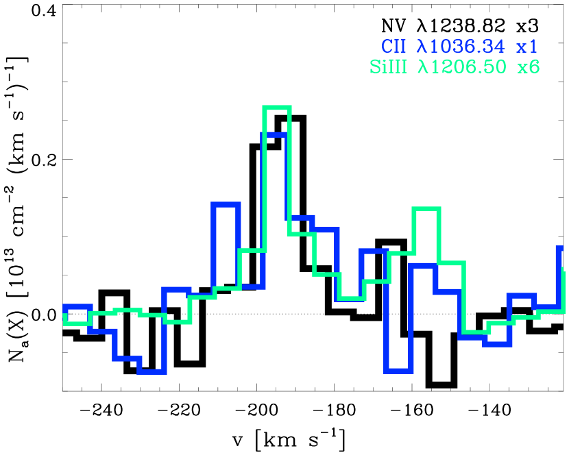
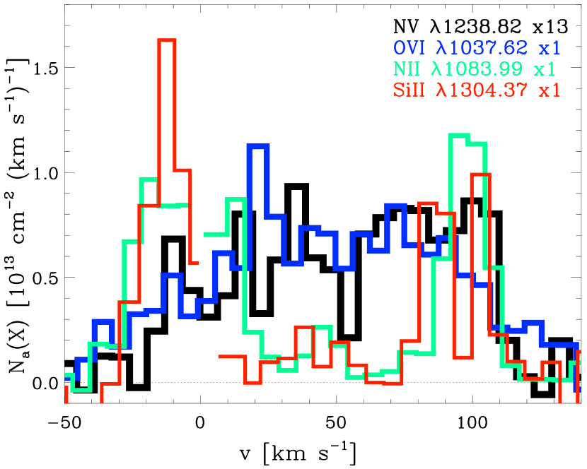
Figure 4.— Apparent column-density profiles of the metal ions relative to $z=0.20258$. Left panel: AOD profiles for the absorber at $z\approx 0.2018$ ($v\approx-190$ ${\rm km\,s}^{-1}$). Note how well high, intermediate, and low ions follow each other. Right panel: AOD profiles for the LLS. Missing data points in the N II and Si II profiles indicate that there is zero-flux at these velocities. Note how well N V and O VI follow each other with little structures in the profiles, while the low and intermediate ions follow each other very well with clearly separated components at about $0$ and $+95$ ${\rm km\,s}^{-1}$.

4.1.2 Ionization

The LLS at $z\approx 0.2026$ shows absorption from atomic to weakly ionized species to highly ionized species. The singly (e.g., C II, Si II) and doubly (e.g., Fe III) ionized species have very similar kinematics, suggesting that they probe the same gas (see Fig. 3). In contrast, the O VI and N V profiles are broad, not following the same kinematics as the low ions. Fig. 4 illustrates this further, where the $N_{a}(v)$ profiles of Si II, N II, O VI, and N V are shown. Over the $[-50,+130]$ ${\rm km\,s}^{-1}$ interval, O VI and N V $N_{a}(v)$ profiles follow each other very well but are quite different from the low-ion profiles. The stronger columns for the weakly ionized gas are between about $[-20,+20]$ ${\rm km\,s}^{-1}$, while at $\sim$45 and 100 ${\rm km\,s}^{-1}$ the columns are much less important. For the high ions, the $N_{a}(v)$ profiles peak in $[+20,+100]$ ${\rm km\,s}^{-1}$ interval. This difference in the kinematics strongly hints at a multiphase gas, where the high ions are produced by a different mechanism than the low ions and/or the low and high ions are not co-spatial.

In order to test these hypotheses, we first use a photoionization model to attempt to reproduce the observed column densities of the low ions and see if such a model can produce significant high-ion columns. We used the photoionization code Cloudy version C07.02 (Ferland et al., 1998) with the standard assumptions, in particular that the plasma exists in an uniform slab and there has been enough time for thermal and ionization balance to prevail. We model the column densities of the different ions through a slab illuminated (on both sides) by the Haardt & Madau (2005, in prep.) UV background ionizing radiation field from quasars and galaxies and the cosmic background radiation appropriate for the redshift $z=0.2026$ ($J_{\nu}(912)=5.4\times 10^{-23}$ erg cm^-2 s^-1 Hz^-1 sr^-1). We also assume a priori solar relative heavy element abundances from Asplund, Grevesse, & Sauval (2006). We do not include the effects of dust on the relative abundances, although we consider this possibility a posteriori. We then vary the ionization parameter, $U=n_{\gamma}/n_{\rm H}=$ H ionizing photon density/total hydrogen number density [neutral + ionized], to search for models that are consistent with the constraints set by the column densities and $b$-values.

The results from the Cloudy simulations for the LLS are shown in Fig. 5 (see also the summary Table 5). The Cloudy simulations stop running when $\log N($H I$)=18.2$ is reached. We adopted a metallicity $[{\rm Z/H}]=-0.6$ within the $1\sigma$ value derived using O I/H I. Smaller metallicities have difficulties in reproducing the column densities of Fe II (and this would be exacerbated if Fe is depleted into dust). In Fig. 5, the yellow region shows the solution $\log U=-3.15\pm 0.10$ that reproduces the S III, Fe III, O I, and Fe II column densities within about 1$\sigma$ (see Table 5). The limits of the other singly ionized species are consistent with this model. This range of $U$ values implies $\log N($H II$)=19.8\pm 0.1$, a density $\log n_{\rm H}=-2.5\pm 0.1$, a temperature $T\simeq 1.1\times 10^{4}$ K. The linear size of the absorber, $L\equiv N({\rm H})/n_{\rm H}$, is 4–12 kpc (a range of values not including the error on $N($H I$)$ and $[{\rm Z/H}]$).

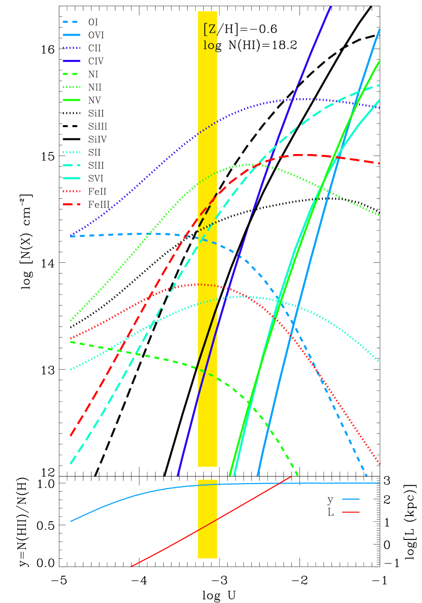
Figure 5.— Top panel: Predicted column densities for the Cloudy photoionization model of the LLS assuming a Haardt-Madau (galaxies+QSOs) spectrum at $z=0.203$. The various lines show the models for each atoms or ions. Relative solar abundances are assumed. The yellow region shows a solution at $\log U=-3.15$ that fits the observations within about $\pm 0.1$ dex for O I, Fe II, Fe III. This model does, however, not produce enough highly ionized species. Although C IV is not observed, we nevertheless show the model prediction as there might be future COS NUV observations of PKS 0312-77. Bottom panel: Variation of the neutral fraction and the path length ($L\equiv N({\rm H})/n_{\rm H}$). For the solution that fits the observations, the fraction of ionized gas is about 98% and the linear scale ranges between 4 and 12 kpc.

Table 5Column densities and Abundances from the Cloudy photoionization model for the absorber at $z\approx 0.2026$

Species	$\log N_{\rm obs}$a	$[{\rm X^{+i}/H^{0}}]^{a}$	$\log N_{\rm model}$b	$[{\rm X^{+i}/H^{0}}]^{b}$
C II	$>14.31$	$>-0.3$	$15.3,15.2$	$+0.7,+0.6$
C IV	$\cdots$	$\cdots$	$12.8,13.3$	$-1.8,-1.3$
N I	$<13.36$	$<-0.7$	$13.1,13.1$	$-0.9,-0.9$
N II	$>14.50$	$>+0.5$	$14.8,14.9$	$+0.8,+0.9$
N V	$13.86\pm 0.04$	$-0.2\pm 0.2$	$10.7,11.4$	$-3.3,-2.6$
O I	$14.17\,^{+0.14}_{-0.22}$	$-0.7\pm 0.3$	$14.3,14.3$	$+0.6,-0.6$
O VI	$14.95\pm 0.05$	$+0.0\pm 0.2$	$7.2,9.8$	$-7.7,-5.1$
Si II	$>14.12$	$>+0.4$	$14.3,14.4$	$+0.5,+0.6$
Si III	$>13.55$	$>-0.2$	$14.3,14.6$	$+0.5,+0.8$
Si IV	$>14.38$	$>+0.6$	$13.1,13.5$	$-0.7,-0.3$
Al III	$<13.15$	$<+0.5$	$12.6,12.9$	$-0.1,+0.2$
S II	$14.1\,^{+0.2}_{-0.3}$	$+0.7\pm 0.3$	$13.7,13.7$	$+0.3,+0.3$
S III	$14.58\pm\,^{0.10}_{0.06}$	$+1.2\pm 0.2$	$14.2,14.4$	$+0.8,+1.0$
S VI	$13.7\,^{+0.2}_{-0.3}$	$+0.3\pm 0.3$	$10.5,11.2$	$-2.9,-2.2$
Fe II	$13.83\pm 0.11$	$+0.1\pm 0.2$	$13.9,13.8$	$+0.2,+0.1$
Fe III	$14.46\pm 0.07$	$+0.8\pm 0.2$	$14.4,14.6$	$+0.7,+0.9$

Note. — $a$: Estimated values for the absorber at $z\approx 0.2026$. $b$: Values from the Cloudy simulation presented in §4.1.2 where the left and right hand-side values are for $\log U=-3.25$ and $-3.05$, respectively.

Although the limit on Si IV is reproduced by this model, it is likely that there is some extra Si IV column not reproduced as the lines are so saturated for this doublet. Both N V and O VI cannot be reproduced with this photoionization model by orders of magnitude (see Table 5). The column density of S VI is more uncertain, but the photoionization also falls short to produce enough column for this ion. Even if we consider only the velocity interval $[-40,+30]$ ${\rm km\,s}^{-1}$, this discrepancy would still exist ($\log N($O VI$)$ = 14.5 over $[-40,+30]$ ${\rm km\,s}^{-1}$). If non-thermal motions dominate the broadening of the N V and O VI profiles, one could imagine that photoionization with a large $U$ could reproduce the observed column densities if one invokes that nitrogen is deficient (see Fig. 5). This would require a much more diffuse gas ($n_{\rm H}<6\times 10^{-5}$ cm^-3) or an intense local source of hard ionizing radiation. The former model, in turn, is ruled out by the inferred size of the absorber, which implies a velocity sheer from Hubble broadening that far exceeds the observed velocity interval.

The broadenings of the O VI and N V profiles are large with $b($O VI$)=59\pm 3$ ${\rm km\,s}^{-1}$ and $b($N V$)=55\pm 10$ ${\rm km\,s}^{-1}$, implying $T<(2$–$3)\times 10^{6}$ K. We note that Tripp et al. (2008) fitted the O VI profiles with two components with $b=48\pm 7$ ${\rm km\,s}^{-1}$ and $35\pm 6$ ${\rm km\,s}^{-1}$, which is still consistent with $T<(2$–$3)\times 10^{6}$ K within the errors. Danforth & Shull (2008) only fitted a single component to the N V and O VI profiles with $b=63\pm 6$ ${\rm km\,s}^{-1}$ and $63\pm 2$ ${\rm km\,s}^{-1}$, respectively. Thom & Chen (2008) fitted the O VI with a single component as well ($b=68\pm 3$ ${\rm km\,s}^{-1}$), but they fitted the N V profiles with several components that follow somewhat the kinematics of N II. In view of the excellent agreement between the O VI and N V $N_{a}(v)$ profiles displayed in Fig. 4, we are confident in our interpretation, i.e. the kinematics of N V and O VI must be similar (and different from the low ions). Our own inspection of the O VI and N V profiles shows that, since the data are quite noisy, a single- or two-component fit produce very similar reduced-$\chi^{2}$. It is quite possible likely that there is more than one component in the high-ion profiles, but that does not rule out the presence of $10^{6}$ K gas (if $b($O VI$)=32$ ${\rm km\,s}^{-1}$ in the individual components and the broadening is mostly due to thermal motions, $T\sim 10^{6}$ K).

From the adopted column densities, the high-ion ratios are: $N($O VI$)/N($N V$)\simeq 13$ and $N($O VI$)/N($S VI$)\simeq 11$–35. The high-ion ratios predicted by collisional ionization equilibrium (CIE) or non-equilibrium collisional ionization (NECI) models (Gnat & Sternberg, 2007) are consistent with these values if $T\sim(3$–$10)\times 10^{5}$ K as long as $N($O VI$)/N($S VI$)\gtrsim 30$. Subsolar (down to $-0.6$ dex) to solar $[{\rm N/O}]$ would be allowed in such models. A future estimate of the C IV column density with the Cosmic Origins Spectrograph (COS) would further constrain this model. For $T<(2$–$3)\times 10^{6}$ K, the H I column density would be $<10^{14.2}$ cm^-2 in CIE or NECI (regardless of the metallicity), which may be accommodated for in the profile fitting presented in §3.2. As both photoionized and collisionally ionized gas are present from $-50$ to $+130$ ${\rm km\,s}^{-1}$, if the gas is co-spatial, it is multiphase.

Although the O VI and N V profiles are broad, they do not appear that broad for such a high column density in the context of models involving radiative cooling flows. Heckman et al. (2002) argue that these models are able to naturally reproduce the relation between $N($O VI$)$ and $b($O VI$)$ measured in various environments. However, using figure 1 in Heckman et al. (2002), an O VI absorber with $\log N($O VI$)=15$ should have $b\simeq 160$ ${\rm km\,s}^{-1}$ in these models, a factor 3 larger than observed here. Furthermore the ratios $N($O VI$)/N($N V$)\simeq 25$–40 and $N($O VI$)/N($S VI$)\simeq 250$–630 in these models are also quite different from the observed ratios (for the O VI/S VI ratio, see Lehner et al., 2006). Hence better physical models might involve shock-ionizations that heat the gas or interfaces between cool ($T\lesssim 10^{4}$ K) and hot ($T>10^{6}$–$10^{7}$ K) plasmas or a diffuse hot gas at $T\lesssim 2\times 10^{6}$ K that has not yet had time to cool.

We can gauge the fraction of the highly ionized gas relative to the neutral gas by estimating the amount of hydrogen in the highly ionized phase from $N_{\rm CI}($H II$)=N($O VI$)/(f_{\rm O\,VI}\,({\rm O/H})_{\odot}10^{[{\rm O/H}]})$ (the subscript “CI” stands for “collisional ionization”), where $f_{\rm O\,VI}=N($O VI$)/N({\rm O})$ is the ionization fraction. For $T\sim(3$–$10)\times 10^{5}$ K, $f_{\rm O\,VI}=0.2$–0.03 if the gas is in CIE or NECI. These $f_{\rm O\,VI}$ values imply $\log N_{\rm CI}($H II$)\simeq(19.0,19.8)-[{\rm O/H}]$. If the metallicity of the O VI-bearing gas is similar to that of the LLS and $T\sim 3\times 10^{5}$ K in the collisionally ionized gas, the H II column density in the highly and photoionized gas would be about the same, implying $N_{\rm tot}($H II$)\gtrsim 10^{20}$ cm^-2 and $N_{\rm tot}($H II$)/N($H I$)\sim 50$. If $T\sim 10^{6}$ K in the collisionally ionized gas, $N_{\rm CI}($H II$)\gtrsim 10^{20.5}$ cm^-2 and $N_{\rm tot}($H II$)/N($H I$)\sim 204$. If the metallicity is much smaller than $-0.7$ dex, then $N_{\rm tot}($H II$)/N($H I$)\gg 54$–200, i.e. the amount of highly ionized gas could be indeed quite large.

4.2. Properties of the Absorber at $z\approx 0.2018$

As we discussed in §3, the absorbers at at $z=0.201798$ and 0.201930 are strongly blended with each other, and the H I column densities in the individual components are somewhat uncertain. Therefore for our analysis we treat these absorbers as a single one at $z\approx 0.2018$ ($v\approx-190$ ${\rm km\,s}^{-1}$ relative to the LLS), and adopt the total column density from our analysis in §3.2, $\log N($H I$)=15.55\,^{+0.19}_{-0.24}$.

The ionization properties of these absorbers appear quite different to the absorber discussed above. The weak N V absorption is narrow and well aligned with Si III and C II, and the AOD profiles for these ions follow each other extremely well (see Fig. 4), suggesting that they arise in a single physical region. The $b$-value of N V is $6.5\pm 2.4$ ${\rm km\,s}^{-1}$, implying $T<7\times 10^{4}$ K. The S/N levels near the O VI absorption profiles are too low to derive any useful $b$-value. If the gas is collisionally ionized, it must be out of equilibrium and has $Z>Z_{\odot}$ according to the calculations of Gnat & Sternberg (2007). The ratio N V/O VI $\sim 0.3$ can be produced in NECI models if $Z>Z_{\odot}$ and $T<3\times 10^{4}$ K (assuming solar relative abundances). This would require a ratio of Si II/Si IV $\sim 5$–10 (consistent with the limit $>0.3$). The ratio C II/Si II would be a factor 2–5 too larger though. However, it is not clear how well these models tackle the low temperature regimes where photoionization becomes important as well.

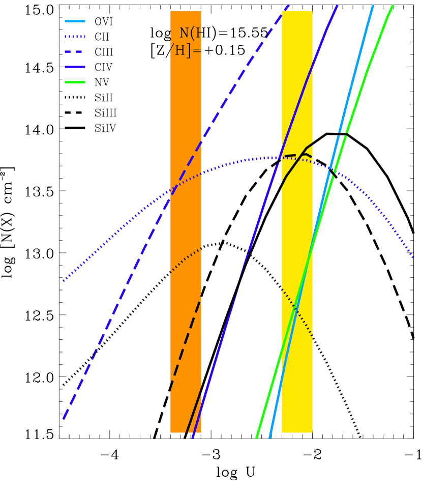
Figure 6.— Similar to Fig. 5 but for the absorber at $z\approx 0.2018$ ($v\approx-190$ ${\rm km\,s}^{-1}$). Note that here the metallicity is a free parameter and was varied to match the column densities of C II, Si II, and Si IV. There are two possible solutions that are shown with the orange and yellow regions. For the smaller $U$ solution, the intermediate and high ions need to be produced in non-equilibrium collisionally ionized gas. The other solution requires supersolar N and O relative to Si and C. For these solutions, the gas is about 100% ionized and the linear scale is $\lesssim 2$–5 kpc.

We therefore explore the possibility that the gas could be solely photoionized. Since the 3$\sigma$ upper limit on O I $\lambda$1302 ($[{\rm O/H}]<+2.0$) is not useful, we let the metallicity be a free parameter in our Cloudy simulations. The calculations were stopped when the H I column density reached $10^{15.55}$ cm^-2 and the metallicity was varied in order to reproduce the observed column densities of C II and Si II (which are the most likely ions to be produced by photoionization in view of their low ionization potentials). Again, the metallicity must be high, $[{\rm Z/H}]=+0.15$ (and at least $[{\rm Z/H}]>-0.2$ when the error on $N($H I$)$ are taken into account) in order to reproduce the column density of Si II and C II (see Fig. 6). For $\log U\simeq-2.15$ (yellow region in Fig. 6), the observed column densities of C II, Si II, and Si IV can be successfully reproduced within the errors. The lower limits on C III and Si III also agree with this model. However, for this value of $U$, supersolar N and O abundances relative to C and Si are required in order to fit N V and O VI. The orange region in Fig. 6 shows another possible solution where $\log U\sim-3.15$: in this case the photoionization produces negligle column densities for all the investigated species but Si II and C II. A combination of photoionization and (non-equilibrium) collisional ionization may produce the observed ions for that solution.

Although it is not entirely clear which ionization processes dominate, for any models, supersolar abundances are required. The linear scale of the gas is also small ($<2$–5 kpc, based on our photoionization model), and any other (local) sources of ionizing radiation will only decrease the size inferred for this absorber. We note a Cloudy simulation where the UV background is dominated solely by QSOs would imply smaller $U$ but even a higher metallicity. The measurement of the C IV column density would provide another constraint in order to test photoionization versus NECI models.

The origin of this absorber is therefore quite different from the LLS in view of the large metallicity difference, that despite the small redshift differences between these two absorbers. Since the gas is 100% ionized, it is unlikely that the sightline probes the gas from a galactic disk. It is more likely associated with some enriched material ejected from a galaxy. The size of the absorber is also much smaller than usually derived in metal-line absorber with $\log N($H I$)<16$ (e.g., Prochaska et al., 2004; Lehner et al., 2006), further suggesting that it is closely connected to a galactic structure.

5. Physical Origin(s) of the Absorbers

5.1. Summary from the Spectroscopic Analysis

Before describing the galaxy survey in the field of view centered on PKS 0312–77, we summarize the possible origins of the absorbers based on the spectroscopic analysis. None of the absorbers originates in the voids of the intergalactic medium where the influence from galaxies is negligible since the gas in these absorbers is metal enriched. These absorbers therefore originate near galaxies, but unlikely through the disk of a spiral or an irregular galaxy since the gas is nearly 100% ionized.

The LLS (traced by the neutral and weakly ionized species) likely probes material associated with the outskirts of a galaxy (e.g. cool galactic halo, or accreting, or outflowing material) or tidal material from an interaction between galaxies. For another LLS at $z\simeq 0.081$ toward PHL 1811 (also a largely ionized absorber with similar $N($H I$)$), a possible origin was tidal debris (Jenkins et al., 2003, 2005). At $z=0$, for the tidally disrupted gas between the SMC and LMC, Lehner et al. (2008) show that this gas can be dominantly ionized despite relatively high H I column density as seen in the present absorber. Below we show that our galaxy survey also supports an interpretation involving tidal debris from a galaxy merger.

There is also a strong absorption in the high ions near the LLS. We showed that this gas cannot be photoionized but is collisionally ionized. The kinematics of the high ions also reveal little connection with the weak ions, except for the fact that the velocity spread of the high- and low-ions (e.g., C II, Si II, Si III) are similar. In view of the difference in the kinematics and the ionization, it is likely that the O VI arises in a large volume of hot gas in which the LLS is embedded. The CIE and NECI models combined with the broadening of N V and O VI allow the gas to be at $T\sim(3$–$10)\times 10^{5}$ K. Such high temperatures could reflect intragroup gas that is cooling, but we show in §4.1.2 that the gas is unlikely in the process of cooling from a hotter phase. However, groups of late-type galaxies may produce cooler intragoup gas (Mulchaey et al., 1996), and we argue below that the O VI absorber may be a tracer of such a plasma. The strong O VI absorber could also be the signature of a hot galactic corona around a galaxy or interacting galaxies. In this scenario, if the O VI-bearing gas is in pressure equilibrium with the LLS, it implies $n_{\rm O\,VI}=n_{\rm LLS}(T_{\rm LLS}/T_{\rm O\,VI})=0.4$–$1.2\times 10^{-4}$ cm^-3, where $n_{\rm LLS}\simeq 31\times 10^{-4}$ cm^-3, $T_{\rm LLS}=10^{4}$ K, and $T_{\rm O\,VI}=(0.3$–$10)\times 10^{5}$ K (see §4.1.2). The cooling time is then $t_{\rm cool}\approx 0.6$–6 Gyr for the O VI-bearing gas. We showed in §4.1.2 that the properties of the O VI absorber are not consistent with a radiatively cooling gas, so it seems more likely that the O VI-bearing gas has been heated to its peak temperature $3\times 10^{5}$ K, and hence $t_{\rm cool}=600$ Myr is more likely. Below we argue that a galactic halo origin appears quite plausible.

Finally, the absorber at $z\approx 0.2018$ ($v\approx-190$ ${\rm km\,s}^{-1}$) with its supersolar metallicity could be associated with a galactic wind or outflow from an enriched galaxy. For example, in our Galaxy, Zech et al. (2008) described a supersolar high-velocity cloud with low $N($H I$)$ ($=10^{16.50}$ cm^-2). The supersolar metallicity of this absorber implies a different origin than the LLS and suggests small-scale variation of the abundances if the absorbers are co-spatial.

5.2. Las Campanas Observations

To perform multi-slit spectroscopy, the field surrounding PKS 0312–77 was first imaged in the R-band with Swope 1 meter telescope at Las Campanas Observatory. Six exposures of 3600 s were acquired on October 1 2002 and another 3 of 1800 s were acquired on October 3 2002 with the SITe3 CCD in direct imaging mode (pixel size 0.435″on a $2048\times 3150$ array). These images were centered on PKS 0312–77 and covered a field of view of $15\arcmin\times 32\arcmin$. The conditions were photometric and the seeing fair. The exposures were taken with a 10″ dither pattern to account for bad pixels and to facilitate the construction of a supersky flat. Full description of the data reduction can be found in Prochaska et al. (2006). A $15.00\arcmin\times 16.67\arcmin$ cut is shown in Fig. 7.

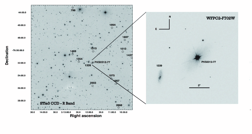
Figure 7.— Left: A $15.00\arcmin\times 16.67\arcmin$ cut from the Las Campanas galaxy survey. Positions of the galaxies and the QSO PKS 0312–77 are shown. Only galaxies within $1200\,\mathrm{km\,s}^{-1}$ of the absorption system are marked (see Table 6). Right: A zoom in on the region very near the QSO using a $36.4\arcsec\times 36.4\arcsec$ cut of a HST WFPC2 image. The galaxy 1339 has only an impact parameter $\rho=38h^{-1}_{70}$ kpc and velocity-offset of 16 ${\rm km\,s}^{-1}$ from the Lyman limit absorbers. The morphology of this galaxy suggests a late-type interacting galaxy (see its optical spectrum in Fig. 8). The outskirts of galaxy 1339 are the likely origin of the LLS and the absorber at $z\approx 0.2018$.

In order to acquire the multi-object spectroscopy, follow-up observations were obtained with the Wide-Field CCD (WFCCD) spectrograph on the 2.5 meter Irénée du Pont telescope at Las Campanas Observatory. We achieve $>90$% completeness to $R\approx 19.5$ within 10′ radius about PKS 0312–77. At $z\approx 0.2$, the survey covers a radius of $\sim 2$ Mpc and is 90% complete for $L\gtrsim 0.5L_{*}$ galaxies. A total of 132 spectra were taken in the field using 5 different slit masks, over the wavelength range 3600–7600 Å. Two to three 1800 s exposures were taken per mask with a spectral resolution of 10 Å and spectral dispersion of 2.8 Å per pixel. The various steps to reduce the data, separate galaxies from stars, and measure the galaxy redshifts are fully described in Prochaska et al. (2006) and we refer the reader to this paper for more information. In total, we have confidently measured redshifts for 105 galaxies.

5.3. Results of the Galaxy Survey

5.3.1 A Galaxy and a Group of Galaxies

In Table 6 we summarize the properties of the galaxies that are situated within $\delta v=c(z-z_{\rm gal})/(1+z)=1200$ ${\rm km\,s}^{-1}$ from the absorbers (and $<1100$ ${\rm km\,s}^{-1}$ from the LLS, see Table 6). Following Prochaska et al. (2006), $\delta v$ is our first criteria for characterizing our sample of galaxies. This cutoff is somewhat arbitrary but allows for peculiar velocities in the largest gravitationally bound galaxies. We also do not impose a priori an impact parameter to allow for large scale structures. The last two columns in Table 6 list the quantities $L_{C}$ and $E_{C}$, which give information about the “type” of the galaxy: early-type galaxies have $E_{C}>0.8$ and $L_{C}<0.4$ and late-type galaxies have $E_{C}<0.8$ and $L_{C}>0.4$. How these quantities are derived is fully explained in Prochaska et al. (2006). Finally, we adopted the absolute magnitude of $L_{*}$, $M_{R}=-21.22$ at $z=0.1$ (Blanton et al., 2003). When we report the $L_{*}$ value from other works in the literature, we corrected it using the magnitude results from Blanton et al. (2003) and our adopted cosmology if necessary.

Table 6Summary of Galaxies Neighboring Absorption Systems

ID	$z_{gal}$	RA	DEC	$R$	$L$	$\Delta\theta$	$\rho$	$E_{C}$	$L_{C}$	$\delta v^{a}$
		(J2000)	(J2000)		($L_{*}$)	($\arcsec$)	($h_{70}^{-1}$ kpc)			(${\rm km\,s}^{-1}$)
1339	0.20264	03 11 57.90	–76 51 55.68	$19.2$	0.66	10.8	38	0.19	0.91	$16$
1515	0.20382	03 11 55.29	–76 50 03.93	$19.9$	0.36	106.8	356	0.03	0.68	$309$
1354	0.19874	03 12 31.87	–76 51 46.31	$19.3$	0.57	125.5	413	0.98	–0.00	$-956$
1469	0.19822	03 12 48.42	–76 50 33.63	$18.5$	1.22	197.5	648	0.30	0.65	$-1087$
2903	0.19821	03 11 54.98	–76 55 33.36	$19.1$	0.67	222.7	731	0.79	0.36	$-1088$
1075	0.20288	03 11 06.85	–76 54 18.78	$18.3$	1.61	221.3	738	0.97	–0.12	$76$
1513	0.20191	03 10 38.19	–76 50 01.76	$20.0$	0.32	283.9	942	0.09	0.68	$-1025$
1007	0.19847	03 10 54.22	–76 55 09.65	$19.7$	0.41	287.5	943	0.45	0.61	$-168$
1427	0.20480	03 10 12.66	–76 50 57.75	$19.3$	0.62	353.2	1185	0.20	0.71	$553$
1697	0.20448	03 10 33.51	–76 48 09.94	$18.6$	1.14	355.1	1190	0.43	0.58	$473$
1894	0.20467	03 11 07.49	–76 46 15.78	$19.0$	0.80	372.2	1248	0.50	0.47	$521$
2668	0.20300	03 10 45.66	–76 58 55.24	$18.7$	1.09	486.1	1623	0.93	0.16	$103$
779	0.20398	03 12 49.91	–76 43 09.44	$18.5$	1.30	553.8	1855	0.95	–0.20	$348$

Note. — The galaxy summary is restricted to those galaxies within $1100\,\mathrm{km\,s}^{-1}$ of the absorption system. The impact parameter refers to physical separation, not comoving. Galaxy redshifts were determined from fitting the four SDSS star and galaxy eigenfunctions to the spectra (see Prochaska et al., 2006). The coefficient of the first eigenfunction $E_{C}$ and a composite of the last three eigenfunctions $L_{C}$ are used to define galaxy type. Early-type galaxies have $E_{C}>0.8$ and $L_{C}<0.4$, while late-type galaxies have $E_{C}<0.8$ and $L_{C}>0.4$. $a$: Velocity separation between the galaxy redshifts and the LLS at $z=0.20258$.

The left-hand side of Fig. 7 shows the galaxy and the QSO positions for the galaxies $\delta v\leq 1100$ ${\rm km\,s}^{-1}$ from the LLS. The galaxy 1339 stands out in view of its proximity to the QSO. For this galaxy, $|\delta v|<100$ ${\rm km\,s}^{-1}$ relative to the LLS and O VI absorption system and the impact parameter is $38h^{-1}_{70}$ kpc, making this galaxy the most likely host of the LLS and O VI  absorber. The next closest galaxy (#1515) is already at $358h^{-1}_{70}$ kpc and $\delta v>200$ ${\rm km\,s}^{-1}$. On the right-hand side of Fig. 7, we zoom in on the region very near the QSO using a $36.4\arcsec\times 36.4\arcsec$ cut of a HST WFPC2 image using the F702W filter (the observations were obtained by PI M. Disney (program 6303), and consist of four exposures totaling 1800 s; we used standard procedures to reduce the WFPC2 images). The HST image goes deeper than our galaxy redshift survey, but except for galaxy 1339 ($0.7L_{*}$), the only galaxies within 100 kpc are less than $0.1L_{*}$ (assuming they are at redshift $z\sim 0.203$). Dwarf galaxies are known to produce outflows (e.g. Martin, 1999) and Stocke et al. (2006) also argue that it is quite likely that many of the responsible galaxies via their outflows and halos for the O VI absorbers may be $<0.1L_{*}$ galaxies. However, since the present O VI absorber is the strongest yet discovered and the linear-scales of the absorbers are quite small ($<12$ kpc, see §4), a scenario where $<0.1L_{*}$ galaxies would be responsible for these strong absorbers does not appear compelling (see also below). Future deeper searches below $0.1L_{*}$ will be needed to uncover the true impact of $<0.1L_{*}$ galaxies on O VI absorbers.

Beyond 300 kpc, there are 5 more galaxies that have $|\delta v|<300$ ${\rm km\,s}^{-1}$ relative to the absorbers at $z\approx 0.2026$ to 0.2030, and 13 with $|\delta v|\lesssim 1100$ ${\rm km\,s}^{-1}$. These galaxies have large impact parameters of $358\leq\rho\leq 1856h^{-1}_{70}$ kpc, consistent with a group of galaxies. Intragroup gas from this group could also be responsible for the O VI absorber. Below, we first review the properties of galaxy 1339 and then address the possible origins of the absorbers.

5.3.2 Properties of Galaxy 1339

The appearance of galaxy 1339 is consistent with a late-type galaxy derived from the $E_{C}$ and $L_{C}$ parameters. A close inspection to the galaxy suggests that it has been subject to a collision or an interaction with another galaxy as there appear to be two bulges separated by about 0.4″ (or $\sim 1h^{-1}_{70}$ kpc), indicating some disruption in this galaxy. In Fig. 8, we show the spectrum of galaxy 1339. The emissions of [O II], [O III], and H$\beta$ with the property $W([$O II${}_{\lambda 3727}])/W([$O III${}_{\lambda 5907}])\approx 1.3$ and $W([$O II${}_{\lambda 3727}])/W({\rm H}\beta)\approx 2.1$ closely mimic the properties of a Sc pec galaxy (e.g., NGC 3690, Kennicutt, 1992a, b) or Sm/Im pec galaxy (e.g., NGC 4194, Kennicutt, 1992b) that is undergoing a close galaxy interaction or merger, confirming our visual inspection of Fig. 7.

Figure 8.— Spectrum of galaxy 1339, the likely host of the Lyman limit system at $z=0.20258$.

Galaxy 1339 is very unlikely to have interacted with another galaxy in a manner like the Galaxy is currently interacting with the LMC and SMC. If that was the case, one would expect to observe a $>0.1L_{*}$ galaxy within a few tens of kpc of galaxy 1339. As the HST images does not reveal any other potential $\gtrsim 0.1L_{*}$ galaxy, the only possibility would be that a galaxy is hidden by the glare of the QSO. We have explored this possibility by subtracting the QSO using a mask to exclude the saturated pixels in the center and surrounding objects. The residual image reveals no serendipitous galaxy or fine structure. Therefore, galaxy 1339 is likely the result of a galaxy merger; perhaps the close interaction between the SMC and LMC will lead these galaxies to a similar fate before being cannibalized by the Milky Way.

The metallicity of the galaxy is an important ingredient to know for comparing the abundances in the absorbers and the likely host galaxy. We can estimate the gas-phase oxygen abundance for galaxy 1339 using the ratios of strong nebular emission lines O II $\lambda$3727, H$\beta$, and O III $\lambda\lambda$4959, 5007 (e.g., Pagel et al., 1978). We assume that the H II regions covered by the spectroscopic slit are chemically homogeneous, and we adopt the calibration between oxygen abundance, $12+\log({\rm O/H})$, and the strong line ratios $R_{23}$ and $O_{32}$ based on the photoionization models of McGaugh (1991) as described in Kobulnicky et al. (1999). We use both the method of flux ratios (not corrected for reddening) and the method of emission line equivalent widths ratios introduced by Kobulnicky & Phillips (2003) that is more robust against reddening; both yield very similar results. We find $12+\log({\rm O/H})=8.90\pm 0.05$. By comparison, the line ratios of the Orion nebula (Baldwin et al., 1991), which might be taken as representative (for emission line studies) of the solar neighborhood, yield $12+\log({\rm O/H})\simeq 8.75$ with a dispersion of about 0.04 dex among multiple sightlines. Hence, the emission lines from galaxy 1339 arise in a region approximately 0.15 dex more metal rich than the solar vicinity in the Milky Way.

Using the H$\beta$ line, we can also roughly estimate the star-formation rate (SFR) in galaxy 1339. From our optical spectrum, we measure $F_{\lambda}({\rm H}\beta)\simeq 3.3\times 10^{-16}$ erg s^-1. At $z=0.203$, this implies $L({\rm H}\beta)\simeq 4.1\times 10^{40}$ erg s^-1 for our adopted cosmology. Assuming no extinction and a standard luminosity ratio $L({\rm H}\alpha)/L({\rm H}\beta)=2.86$, we find $L({\rm H}\alpha)\approx 4.1\times 10^{40}$ erg s^-1. Using Kennicutt (1989) and assuming an extinction of about 1 magnitude, the SFR is $2\pm 1$ $M_{\odot}$ yr^-1, which is roughly consistent with a $\sim$$L_{*}$ galaxy. Hence while galaxy 1339 is not a starburst, it nevertheless sustains star formation, allowing the possibility of stellar feedback, which can produce galactic outflows. We also note that it is quite possible that burst of star formation may have occurred several tens to hundreds of Myr before the observed epoch, leaving open the possibility of violent star formation and mass ejection in the past. This conjecture is supported if galaxy 1339 was subject to a galaxy merger as these events are known to create new burst of star-formations (Larson & Tinsley, 1978; Barton et al., 2007; de Mello et al., 2007).

5.4. Origins of the LLS and $z\approx 0.2018$ Absorber

In view of its properties and impact parameter, galaxy 1339 is a very likely candidate for the origin of the LLS and the absorber at $z\approx 0.2018$ ($v\approx-190$ ${\rm km\,s}^{-1}$). The supersolar metallicity of that galaxy is (remarkably) the same as the one derived for the absorber at $z\approx 0.2018$. The high velocity of the absorber relative to the galaxy velocity ($\delta v=178$–211 ${\rm km\,s}^{-1}$) fits nicely in a scenario involving a galactic wind or outflow from the galaxy. As we show above that star formation is occurring in that galaxy, galactic feedback involving supernovae and stellar winds is quite possible. According to the recent simulations of feedback within cosmological models, a galactic wind may travel on physical distances of 60–100 kpc (Oppenheimer & Davé, 2008a), consistent with the impact parameter of 38 kpc for galaxy 1339. In these models, even $\sim$$L_{*}$ galaxies may produce such outflows.

The velocity offset between the LLS and the galaxy is small ($|\delta v|\simeq 16$ ${\rm km\,s}^{-1}$), suggesting it is bound to the galaxy if projection effects are negligible. Because there is strong evidence that galaxy 1339 is the result of a galaxy merger, it appears reasonable to hypothesize that the LLS traces some leftover debris from the merger. It is interesting to note that the physical distance of the LLS from galaxy 1339, linear size, and H I column density are in fact very similar to recently found H I clouds in the halo of M 31 (Thilker et al., 2004) and in the M81/M82 group (Chynoweth et al., 2008). These clouds are thought to be the extragalactic counterparts of the high-velocity clouds (HVCs) observed in the Galactic halo (e.g., see review by Wakker, 2001). Tidal disruption is also the most obvious origin considered for the H I-halo clouds near M31 and M81/M82 galaxies (Thilker et al., 2004; Chynoweth et al., 2008), especially for the M81/M82 group, which in contrast of M31 is undergoing a strong galactic interaction. Yet neither for the present absorber nor for these other nearby galaxies, other scenarios can be entirely rejected (e.g., condensation of galactic halo material or even outflows several tens or hundreds of Myr before the observed epoch).

The metallicity of the LLS is quite different from that of the absorber at $z\approx 0.2018$ and the galaxy itself. First, we note that the metallicity of galaxy 1339 is unlikely to be homogeneous, especially if it resulted from a recent merger. The different metallicity may arise if the galaxies that merged had different metallicity and/or the leftover debris were mixed with more pristine gas. The difference in metallicity is also indicative of poor metal mixing on galactic-scale structure of tens of kpc. Evidence for poor metal mixing in the $\lesssim 100$ kpc halo of galaxies is also observed at lower redshift in our own Galactic halo (e.g., Wakker, 2001; Collins et al., 2003; Tripp et al., 2003), in the Magellanic system (Gibson et al., 2000; Lehner et al., 2008, N. Lehner et al. 2009, in prep.), and at higher $z$ in other LLS (Prochter et al., 2008), suggesting it is a systematic property of galactic halos (see also Schaye et al., 2007).

We noted above that the O VI-bearing and the LLS could be in pressure equilibrium if they are spatially coincident (see §5.5), then the LLS could be pressure confined by coronal gas traced by the high-ion absorber. Even if the LLS is not pressure confined, the lifetime of such a cloud with the properties derived in §4.1.2 would be about 0.3–0.8 Gyr using the expansion-time equation given by Schaye et al. (2007). It is reasonable, therefore, to associate the LLS with debris from a merger that is just ending and has been happening on the timescale of $\lesssim 1$ Gyr.

5.5. Origin(s) of the Strong O VI Absorber

In the picture presented above, the O VI/N V-bearing gas may represent a hot, collisionally ionized gas about galaxy 1339 as the O VI absorption revealed in Galactic halo sightlines (Savage et al., 2003; Sembach et al., 2003) or about interacting galaxies like the O VI absorption observed toward the LMC or SMC (Howk et al., 2002b; Hoopes et al., 2002; Lehner & Howk, 2007). However, there is also a group of galaxies with $358\leq\rho\leq 1856h^{-1}_{70}$ kpc. It is therefore possible that the O VI absorption is so strong and broad because it probes the large-scale gravitational structures inhabited by the galaxies summarized in Table 6. We explore now if the properties of the O VI absorber compared to other absorbers and to results from cosmological simulations allow us to differentiate between these two scenarios.

Many aspects of feedback are still too complex to reliably model (e.g., metal cooling, non-equilibrium ionization effects) and simulations often lack the spatial and mass resolutions to resolve the supernova environment. Nevertheless, recent simulations attempt to model galactic outflows in a cosmological context, showing that feedback is a necessary ingredient and galactic winds are required to match the low-column O VI absorber density (e.g., Cen & Ostriker, 2006). Oppenheimer & Davé (2008b) specifically investigated the origin(s) of the O VI absorbers in Gadget-2 cosmological simulations that use a variety of physics inputs and include galactic outflows with various strengths. They found that strong O VI absorbers are usually collisionally ionized, but also are found in multiphase gas and may be misaligned relative to the low ions as the present O VI absorber. In their models, strong O VI absorbers trace the outskirts of the halos, while absorbers with $\log N($O VI$)\gtrsim 15$ trace metals in galactic halo fountains within the virial radius. In their models, galactic winds travel distances of $\lesssim 100$ kpc, but do not escape the galaxy halo and fall back down in a “halo fountain” on recycling timescales $\leq 2$ Gyr (Oppenheimer & Davé, 2008a). According to figure 12 in Oppenheimer & Davé (2008b), $\gtrsim 0.3M_{*}$ galaxies may recycle absorbers with $\log N($O VI$)\sim 15$ within $\sim$1 Gyr. Above we argue that the absorber $z\approx 0.2018$ might be evidence for a galactic wind, supporting further this interpretation. Therefore, the present strong O VI absorber supports findings of Oppenheimer & Davé (2008b).

From an observational perspective, the properties of the O VI absorber are quite similar to another very strong O VI absorber for which galaxy information exists: Toward PKS 0405–123, a strong O VI absorber with $\log N($O VI$)=14.78$ and $\log N($N V$)=13.89$ was detected at $z=0.16710$ (Chen & Prochaska, 2000; Prochaska et al., 2004; Williger et al., 2006). The full velocity extents of the main O VI and N V absorption are also quite similar with $\Delta v\approx 150$ ${\rm km\,s}^{-1}$. Both absorbers exhibit two distinct phases: (i) a photoionized gas at $T\sim 10^{4}$ K and (ii) a hot ($T\sim 2\times 10^{5}$–$10^{6}$ K), collisionally ionized gas associated with O VI, N V, and S VI absorption. For both absorbers, velocity offsets from velocity of the host galaxy are small, suggesting that both gas phases are bound to the galaxy. The properties of the galaxies have, however, some key differences. First, in the field about PKS 0405–123, the likely host galaxy is much brighter, with $L\sim 3.4L_{*}$. Secondly, there is no evidence for a group of galaxies within 3 Mpc of PKS 0405–123. In view of these properties, a galactic halo origin rather than intragroup medium was strongly favored for the O VI absorber at $z\simeq 0.1671$ toward PKS 0405–123 (Prochaska et al., 2006).

Other strong O VI absorbers have been found (e.g., Tripp et al., 2008), but they are rare, and even more so with close spectroscopically identified galaxies. In their survey of the very local Universe ($z<0.017$), Wakker & Savage (2008) reported a strong O VI absorber with $\log N($O VI$)=14.63\pm 0.15$. This absorber has a $2.1L_{*}$ galaxy at $\rho\simeq 62h^{-1}_{70}$ kpc and with $\delta v=100$ ${\rm km\,s}^{-1}$. This suggests that strong O VI absorbers are generally found near $>L_{*}$ galaxies. On the other hand, not all galaxies with $\rho\lesssim 100h^{-1}_{70}$ kpc have strong O VI absorption: the LLS at $z=0.08$ has two S0 galaxies with $\rho\simeq 34$ and $87h^{-1}_{70}$ kpc but no O VI absorption (Jenkins et al., 2005); at $z<0.02$, several H I absorbers have no O VI or weak O VI absorption for galaxies with $\rho\lesssim 100h^{-1}_{70}$ kpc (Wakker & Savage, 2008), and at $z<0.15$, Stocke et al. (2006) found two-thirds of the O VI non-detections are found within $1h^{-1}_{70}$ Mpc of the nearest galaxy. The absence of strong O VI absorption within 100 kpc of a galaxy is, however, not entirely surprising: the detection rate of O VI absorption (irrespective of its strength) at such an impact parameter is less than 50% (Stocke et al., 2006; Wakker & Savage, 2008). The detection probability can be understood if the O VI-bearing gas is patchy and distributed in complicated sheet-like structures (Howk et al., 2002a), and because the finite distances that metals can reach once ejected from galaxies (Tumlinson & Fang, 2005; Stocke et al., 2006).

Table 7Variety of LLS and “Associated” O VI Absorbers at $z\lesssim 0.2$

Sightline	$z_{\rm LLS}$	$\log N($H I$)$	$\log N_{\rm OVI}$	$[{\rm Z/H}]_{\rm LLS}$	Likely host galaxy	Possible Origin(s)	Possible Origin(s)	Ref.
					$\delta v,\rho,L$	LLS	O VI
					(${\rm km\,s}^{-1}$, kpc, $L_{*}$)
PKS 0405–123	0.16710	$16.5$	$14.8$	$-0.3$	$-15,108,3.4$	galactic halo	galactic halo	1
PKS 1302–102	0.09847	$17.0$	$14.0$	$\lesssim-1.6$	$-354,65,0.2$	outflow/inflow?	outflow/inflow?	2
PHL 1811	0.08092	$18.0$	$<13.2$	$-0.2$	$+36,34,0.5$	tidal debris/wind	$\cdots$	3
PKS 0312–77	0.20258	$18.3$	$15.0$	$-0.6$	$+16,38,0.7$	merger debris	galactic halo/intragroup	4

Note. — PKS 0405–123: There are two galaxies (the other is $\lesssim 0.1L_{*}$) within 108 kpc. All the other galaxies are at $>3$ Mpc (sensitivity of the survey is $0.1L_{*}$).

PKS 1302–102: The large $\delta v$ requires extremely large outflow/inflow for a small galaxy. Ten ($0.1L_{*}\lesssim L\lesssim 5L_{*}$) galaxies are found at $\rho\lesssim 800$ kpc and with $100\lesssim|\delta v|\lesssim 600$ ${\rm km\,s}^{-1}$, which might suggest the intragroup medium as the origin of the LLS and O VI (sensitivity of the survey is $\sim 0.2L_{*}$).

PHL 1811: Another $0.5L_{*}$ galaxy is found with $\delta v=146$ ${\rm km\,s}^{-1}$ and at 87 kpc.

PKS 0312–77: See this paper.

References: (1) Prochaska et al. (2004, 2006); (2) Cooksey et al. (2008); (3) Jenkins et al. (2003, 2005); (4) this paper.

While Oppenheimer & Davé (2008b) relate collisionally ionized O VI absorbers to HVCs or IVCs observed in the Milky Way halo, such strong O VI is not observed in the FUSE O VI survey of the Galactic halo (Wakker et al., 2003; Savage et al., 2003; Sembach et al., 2003). Strong O VI absorption is generally related to the “thick” disk of the Galaxy, but thick disk material cannot have been probed by this sightline. On the other hand, the O VI might be so strong because it probes the halo of a galaxy merger, which possibly produced in the past a strong burst of star formation, and hence strong galactic feedback. As we have alluded to above, galaxy 1339 may be an evolved system of the fate awaiting the SMC-LMC system, two sub-$L_{*}$ galaxies. For the O VI  absorption toward the LMC stars, Howk et al. (2002b) and Lehner & Howk (2007) argue that the O VI  absorption probes a hot halo and feedback phenomena associated with the LMC. The LMC O VI column densities are generally smaller than 14.5 dex (see summary table 7 in Lehner & Howk, 2007). However, these sightlines only pierce one side of the halo of the LMC as the background targets are stars. In the SMC, one line of sight has $\log N($O VI$)\approx 14.9$ and several have $\log N($O VI$)>14.6$ (Hoopes et al., 2002). The enhancement is related to the stellar activity within the SMC and it is not clear how much of the O VI absorption arises in the SMC halo versus the SMC disk. Yet, it is not outside of the realm of possibility that a sightline piercing through the combined halo of these galaxies could probe very strong O VI absorption. We also note some shared properties between extragalactic strong O VI absorbers and O VI  absorption from gas related to galactic environments: (i) the O VI profiles generally appear featureless while the low ions show complicated narrow absorption profiles, and (ii) absorption from both the high and low ionization species are observed over the entire range of velocities where the O VI absorption is observed (e.g., Lehner & Howk, 2007; Howk et al., 2002b).

Hence it seems possible from both observational and theoretical points of view that the strong O VI absorber could trace coronal gas in the halo of galaxy 1339, especially if this galaxy is the result of a recent galaxy merger. However, this may not be the sole explanation. In their models, Oppenheimer & Davé (2008b) discuss that strong O VI absorbers may also be related to intragroup medium. The present group of galaxies must be quite different from those where $\gtrsim 10^{7}$ K ($\gtrsim 1$ keV) intragroup gas was discovered. Mulchaey et al. (1996) found that X-ray detected systems contain at least one bright elliptical galaxy ($\gtrsim 4L_{*}$) and have generally a high percentage of early-type galaxies. With 60% of late-type galaxies and the brightest early-type galaxy having $L\approx 1.6L_{*}$, neither of these conditions is satisfied for the present sample of galaxies. However, Mulchaey et al. (1996) also speculate that the absence of hot, diffuse intragroup medium in spiral-rich groups may simply mean that the hot gas was too cool to detect with ROSAT, i.e. it would have a temperature less than 0.3 keV ($T\lesssim 3\times 10^{6}$ K). This is in fact consistent with the broadenings of the O VI and N V profiles. As the instantaneous radiative cooling is $t_{\rm cool}\sim(0.2$–$0.4)(n/10^{-3}\,{\rm cm}^{-3})^{-1}$ Gyr for a $10^{6}$ K gas (e.g., Gnat & Sternberg, 2007), if the density is low enough, the gas can remain highly ionized for a very long time. Therefore, we cannot reject a diffuse intragroup gas at $T\sim 0.1$–0.3 keV for the origin of the O VI absorber. As Tripp et al. (2008) show, the profiles of O VI can be fitted with two components, and it is in fact quite possible that the strong O VI absorber along PKS 0312–77 may actually trace gas from two different physical regions.

6. The LLS and Strong O VI Absorbers at Low $z$: Tracers of Circumgalactic Environments

In Table 7, we summarize the current knowledge of LLS-galaxies connection in the low redshift Universe. The sample of LLS observed at high spectral resolution (allowing, e.g., to derive accurate H I and metal-ion column densities) and with galaxy information is still small. Nevertheless this table demonstrates that LLS are not related to a single phenomenon. Galactic feedback, accretion of material, tidal or merger debris are all a possibility, without mentioning the possibility that there may be some unrelated clouds to the galaxy such as low-mass dark matter halos (however, LLS must still be related to some galaxy activity as the gas is generally – but not always – metal enriched). While the physical origins of the LLS may be diverse, LLS have also common characteristics. First it appears obvious that the LLS are not the traditional interstellar gas of star-forming galaxies as DLAs could be. Second the LLS are often too metal-rich to be pristine intergalactic gas. Therefore, and thirdly, the LLS representing the IGM/galaxy interface is well supported with the current observations and knowledge. The characteristics of the LLS are also similar to HVCs seen in the halo of the Milky Way (see, e.g., Richter et al., 2008) and found near other nearby galaxies (M31, LMC, M81/M82 Thilker et al., 2004; Staveley-Smith et al., 2003; Lehner & Howk, 2007; Chynoweth et al., 2008). We note that the velocities of LLS relative to the host galaxy may not appear to be “high” (as for the LLS toward PKS 0312–77) on account of projection effects but also simply because in our own Galaxy, halo clouds not moving at high velocities cannot be separated from disk material moving at the same velocities (and indeed some of H I clouds observed in the halo of other galaxies do not systematically show large velocity departures from the systemic velocity of the galaxy).

This work combined with previous studies also suggest that strong O VI absorbers generally trace circumgalactic gas rather than the WHIM, supporting the findings from the cosmological simulations by Oppenheimer & Davé (2008b). We, however, emphasize that neither in the simulations nor in the observations at low $z$ the threshold on $N($O VI$)$ is well defined. For example, Howk et al. (2008) discussed a strong O VI absorber ($\log N($O VI$)\approx 14.50$, currently in the top 10% of the strongest O VI absorber at $z<0.5$) that is more likely to be dominantly photoionized and may not be directly associated with galaxies. However, the three strong O VI absorbers discussed above are all associated with a LLS, while the one studied by Howk et al. (2008) is not. The association of strong O VI absorbers with LLS suggests these systems trace galactic and not intergalactic structures.

The current sample, where detailed information on the properties of the absorbers and galaxies in the field of view is available, is still small, but should increase in the near future. Future observations with COS coupled with ground based and HST imaging observations of the field of view of QSOs will open a new door for studying the QSO absorbers-galaxies connection at low $z$. Attempt to systematically derive the metallicities and SFRs of the possible host galaxies and their morphologies may help disentangling the various origins of the absorbers.

7. Summary

We have presented multi-wavelength observations of the absorbing material at $z\approx 0.203$ along the QSO PKS 0312–77 and its field of view with the goal of exploring the properties of the Lyman limit system and the strongest O VI absorber yet discovered in the low redshift Universe, and the connection between the absorbers and their environments (i.e. galaxies). The main results of our analysis are as follows:

1. Using $N($O I$)/N($H I$)$ combined with a photoionization model, we show that the LLS at $z=0.20258$ has a metallicity of about $-0.6$ dex solar. At slightly lower redshift ($z\approx 0.2018$, velocity separation of about $-190$ ${\rm km\,s}^{-1}$), another absorber is detected with a much higher metallicity ($[{\rm Z/H}]=+0.15$) according to our ionization models, implying that these two absorbers have different origins. The metallicity variation implies poor mixing of metals on galactic scale as observed in lower and higher redshift galactic halos.

2. The gas in both absorbers at $z\approx 0.2018$ and $z=0.20258$ is nearly 100% photoionized. But only from $-70$ to $+150$ ${\rm km\,s}^{-1}$ ($0.2023\lesssim z\lesssim 0.2030$), extremely strong O VI absorption ($W_{\rm O\,VI\lambda 1032}=493\pm 40$ mÅ, $\log N($O VI$)=14.95\pm 0.05$) is observed. Associated with the O VI, there are a detection of N V and a tentative detection of S VI. At $z\approx 0.2018$, narrow N V absorption is detected, more consistent with the N V originating from photoionized gas or in collisionally ionized gas far from equilibrium.

3. Using Cloudy photoionization models, we show that the high ions at $-70\lesssim v\lesssim+150$ ${\rm km\,s}^{-1}$ cannot be photoionized. CIE or non-equilibrium models can reproduce the observed high-ion ratios if the gas temperature is $T\sim(3$–$10)\times 10^{5}$ K. The broadenings of O VI and N V are consistent with such high temperatures. The high-ion profiles are broad, while the low-ion profiles reveal several narrow components. The full velocity extents of the low and high ions are, however, quite similar, as usually observed in galactic environments. If the gas of the LLS and O VI absorber is cospatial, it is multiphase, with the photoionized gas embedded within the hot, collisionally highly ionized gas.

4. Our galaxy survey in the field of view of PKS 0312–77 shows that there are thirteen $0.3\lesssim L/L_{*}\lesssim 1.6$ galaxies at $\rho\lesssim 2h^{-1}_{70}$ Mpc and velocity offset from the absorbers $|\delta v|\lesssim 1100$ ${\rm km\,s}^{-1}$, implying a group of galaxies near the O VI absorber at $z\approx 0.203$. The closest galaxy (#1339, a $0.7L_{*}$ galaxy) has only an impact parameter of $38h^{-1}_{70}$ kpc and is offset by 16 ${\rm km\,s}^{-1}$ from the LLS at $z=0.20258$. There is no evidence of other $\gtrsim 0.1L_{*}$ galaxies within $100h^{-1}_{70}$ kpc. From both a visual inspection of its morphology and its spectral classification (Sc or Irregular), galaxy 1339 appears to have resulted from a galaxy merger. Using diagnostics from the emission lines, we show that the metallicity of galaxy 1339 is supersolar ($[{\rm Z/H}]_{\rm gal}=+0.15\pm 0.05$) and that star formation occurs at a rate $2\pm 1$ M_⊙ yr^-1.

5. Merger debris of galaxy 1339 is a very likely possibility for the origin of the LLS. Outflowing material from galaxy 1339 is also very probable the origin for the supersolar absorber at $z\approx 0.2018$. The strong O VI absorber may be a tracer of a galaxy halo fountain. However, the presence of a group dominated by late-type galaxies and with no very bright early-type galaxy may as well suggest that the O VI absorber probes diffuse intragroup medium at $T\lesssim 10^{6}$ K.

6. Compiling our results with other studies, it is apparent that while the origin of the LLS is not unique (and likely includes galactic feedback, galactic halo, accreting material,…), they must play an important role in the formation and evolution of galaxies, and are among the best probes to study the galaxy-IGM interface over cosmic time. Strong O VI absorbers associated with LLS appear good tracers of enrichment in galactic halos and intragroup medium rather than the WHIM itself.

References

- Asplund, Grevesse, & Sauval (2006) Asplund M., Grevesse N., & Sauval A. J. 2006, CoAst, 147, 76
- Baldwin et al. (1991) Baldwin, J. A., Ferland, G. J., Martin, P. G., Corbin, M. R., Cota, S. A., Peterson, B. M., & Slettebak, A. 1991, ApJ, 374, 580
- Barton et al. (2007) Barton, E. J., Arnold, J. A., Zentner, A. R., Bullock, J. S., & Wechsler, R. H. 2007, ApJ, 671, 1538
- Bergeron & Boissé (1991) Bergeron, J., & Boissé, P. 1991, A&A, 243, 344
- Bertone et al. (2007) Bertone, S., De Lucia, G., & Thomas, P. A. 2007, MNRAS, 379, 1143
- Blanton et al. (2003) Blanton, M. R., et al. 2003, ApJ, 592, 819
- Bouché (2008) Bouché, N. 2008, MNRAS, 389, L18
- Bowen et al. (2008) Bowen, D. V., et al. 2008, ApJS, 176, 59
- Bowen et al. (2002) Bowen, D. V., Pettini, M., & Blades, J. C. 2002, ApJ, 580, 169
- Cen & Ostriker (1999) Cen, R., & Ostriker, J. P. 1999, ApJ 514, 1
- Cen & Ostriker (2006) Cen, R., & Ostriker, J. P. 2006, ApJ, 650, 560
- Chen & Lanzetta (2003) Chen, H.-W., & Lanzetta, K. M. 2003, ApJ, 597, 706
- Chen et al. (2001) Chen, H.-W., Lanzetta, K. M., Webb, J. K., & Barcons, X. 2001, ApJ, 559, 654
- Chen & Prochaska (2000) Chen, H.-W., & Prochaska, J. X. 2000, ApJ, 543, L9
- Churchill et al. (2005) Churchill, C. W., Kacprzak, G. G., & Steidel, C. C. 2005, IAU Colloq. 199: Probing Galaxies through Quasar Absorption Lines, 24
- Chynoweth et al. (2008) Chynoweth, K. M., Langston, G. I., Yun, M. S., Lockman, F. J., Rubin, K. H. R., & Scoles, S. A. 2008, AJ, 135, 1983
- Collins et al. (2003) Collins, J. A., Shull, J. M., & Giroux, M. L. 2003, ApJ, 585, 336
- Cooksey et al. (2008) Cooksey, K. L., Prochaska, J. X., Chen, H.-W., Mulchaey, J. S., & Weiner, B. J. 2008, ApJ, 676, 262
- Danforth & Shull (2008) Danforth, C. W., & Shull, J. M. 2008, ApJ, 679, 194
- Davé et al. (1999) Davé, R., Hernquist, L., Katz, N., & Weinberg, D. H. 1999, ApJ, 511, 521
- de Mello et al. (2007) De Mello, D. F., Smith, L. J., Sabbi, E., Gallagher, J.S., Mountain, M., & Harbeck, D. R. 2007, AJ, 135, 548
- Dixon et al. (2007) Dixon, W. V. et al. 2007, PASP, 119, 527
- Ferland et al. (1998) Ferland, G. J., Korista, K. T., Verner, D. A., Ferguson, J. W., Kingdon, J. B., & Verner, E. M. 1998, PASP, 110, 761
- Fitzpatrick & Spitzer (1997) Fitzpatrick, E. L., & Spitzer, L. J. 1997, ApJ, 475, 623
- Gibson et al. (2000) Gibson, B. K., Giroux, M. L., Penton, S. V., Putman, M. E., Stocke, J. T., & Shull, J. M. 2000, AJ, 120, 1830
- Gnat & Sternberg (2007) Gnat, O., & Sternberg, A. 2007, ApJS, 168, 213
- Heckman et al. (2002) Heckman, T. M., Norman, C. A., Strickland, D. K., & Sembach, K. R. 2002, ApJ, 577, 691
- Henry, Edmunds, Köppen (2000) Henry R. B. C., Edmunds M. G., & Köppen J. 2000, ApJ, 541, 660
- Howk et al. (2008) Howk, J. C., Ribaudo, J., Lehner, N., Prochaska, J. X., & Chen, H.-W. 2008, MNRAS, submitted
- Howk et al. (2002a) Howk, J. C., Savage, B. D., Sembach, K. R., & Hoopes, C. G. 2002a, ApJ, 572, 264
- Howk et al. (2002b) Howk, J. C., Sembach, K. R., Savage, B. D., Massa, D., Friedman, S. D., & Fullerton, A. W. 2002b, ApJ, 569, 214
- Hoopes et al. (2002) Hoopes, C. G., Sembach, K. R., Howk, J. C., Savage, B. D., & Fullerton, A. W. 2002, ApJ, 569, 233
- Impey et al. (1999) Impey, C. D., Petry, C. E., & Flint, K. P. 1999, ApJ, 524, 536
- Jenkins et al. (2000) Jenkins E. B., et al. 2000, ApJ, 538, L81
- Jenkins et al. (2005) Jenkins, E. B., Bowen, D. V., Tripp, T. M., & Sembach, K. R. 2005, ApJ, 623, 767
- Jenkins et al. (2003) Jenkins, E. B., Bowen, D. V., Tripp, T. M., Sembach, K. R., Leighly, K. M., Halpern, J. P., & Lauroesch, J. T. 2003, AJ, 125, 2824
- Kennicutt (1989) Kennicutt, R. C., Jr. 1989, ApJ, 344, 685
- Kennicutt (1992a) Kennicutt, R. C., Jr. 1992a, ApJ, 388, 310
- Kennicutt (1992b) Kennicutt, R. C., Jr. 1992b, ApJS, 79, 255
- Kobulnicky et al. (1999) Kobulnicky, H. A., Kennicutt, R. C., Jr., & Pizagno, J. L. 1999, ApJ, 514, 544
- Kobulnicky & Phillips (2003) Kobulnicky, H. A., & Phillips, A. C. 2003, ApJ, 599, 1031
- Lanzetta et al. (1995) Lanzetta, K. M., Bowen, D. V., Tytler, D., & Webb, J. K. 1995, ApJ, 442, 538
- Larson & Tinsley (1978) Larson, R. B., & Tinsley, B. M. 1978, ApJ, 219, 46
- Lehner & Howk (2007) Lehner, N., & Howk, J. C. 2007, MNRAS, 377, 687
- Lehner et al. (2008) Lehner, N., Howk, J. C., Keenan, F. P., & Smoker, J. V. 2008, ApJ, 678, 219
- Lehner et al. (2003) Lehner N., Jenkins E. B., Gry C., Moos H. W., Chayer P., Lacour S. 2003, ApJ, 595, 858
- Lehner et al. (2007) Lehner, N., Savage, B. D., Richter, P., Sembach, K. R., Tripp, T. M., & Wakker, B. P. 2007, ApJ, 658, 680
- Lehner et al. (2006) Lehner, N., Savage, B. D., Wakker, B. P., Sembach, K. R., & Tripp, T. M. 2006, ApJS, 164, 1
- Lindler (2003) Lindler, D. 2003, CALSTIS Reference Guide v7.2), (Greenbelt:NASA)
- Lu et al. (1998) Lu, L., Sargent, W. L. W., Savage, B. D., Wakker, B. P., Sembach, K. R., & Oosterloo, T. A. 1998, AJ, 115, 162
- Martin (1999) Martin, C. L. 1999, ApJ, 513, 156
- McGaugh (1991) McGaugh, S. S. 1991, ApJ, 380, 140
- Ménard & Chelouche (2008) Ménard, B., & Chelouche, D. 2008, MNRAS, in press [arXiv:0803.0745]
- Morton (2003) Morton, D. C. 2003, ApJS, 149, 205
- Mulchaey et al. (1996) Mulchaey, J. S., Davis, D. S., Mushotzky, R. F., & Burstein, D. 1996, ApJ, 456, 80
- Osterbrock (1989) Osterbrock, D. E. 1989, “Astrophysics of gaseous nebulae and active galactic nuclei”, University Science Books
- Oppenheimer & Davé (2008a) Oppenheimer, B. D., & Davé, R. 2008a, MNRAS, 387, 577
- Oppenheimer & Davé (2008b) Oppenheimer, B. D., & Davé, R. A. 2008b, MNRAS, submitted, arXiv:0806.2866
- Pagel et al. (1978) Pagel, B. E. J., Edmunds, M. G., Fosbury, R. A. E., & Webster, B. L. 1978, MNRAS, 184, 569
- Penton et al. (2002) Penton, S. V., Stocke, J. T., & Shull, J. M. 2002, ApJ, 565, 720
- Prochaska et al. (2004) Prochaska, J. X., Chen, H.-W., Howk, J. C., Weiner, B. J., & Mulchaey, J. 2004, ApJ, 617, 718
- Prochaska et al. (2006) Prochaska, J. X., Weiner, B. J., Chen, H.-W., & Mulchaey, J. S. 2006, ApJ, 643, 680
- Prochter et al. (2008) Prochter, G. E., Prochaska, J. X., O’Meara, J. M., Burles, S., & Berstein, R. A. 2008, ApJ, submitted
- Proffitt et al. (2002) Proffitt, C., et al. 2000, STIS Instrument Handbook, v6.0, (Baltimore:STScI)
- Rao et al. (2003) Rao, S. M., Nestor, D. B., Turnshek, D. A., Lane, W. M., Monier, E. M., & Bergeron, J. 2003, ApJ, 595, 94
- Richter et al. (2008) Richter, P., Charlton, J. C., Fangano, A. P. M., Bekhti, N. B., & Masiero, J. R. 2008, ApJ, submitted
- Rauch (1998) Rauch, M. 1998, ARA&A, 36, 267
- Savage et al. (1990) Savage, B. D., Edgar, R. J., & Diplas, A. 1990, ApJ, 361, 107
- Savage & Sembach (1991) Savage, B. D., & Sembach, K. R. 1991, ApJ, 379, 245
- Savage et al. (2003) Savage, B. D., et al. 2003, ApJS, 146, 125
- Schaye et al. (2007) Schaye, J., Carswell, R. F., & Kim, T.-S. 2007, MNRAS, 379, 1169
- Sembach et al. (2001) Sembach, K. R., Howk, J. C., Savage, B. D., & Shull, J. M. 2001, AJ, 121, 992
- Sembach et al. (2003) Sembach, K. R., et al. 2003, ApJS, 146, 165
- Spitzer (1978) Spitzer, L. 1978, “Physical processes in the interstellar medium”, New York Wiley-Interscience
- Steidel (1993) Steidel, C. C. 1993, Galaxy Evolution. The Milky Way Perspective, 49, 227
- Staveley-Smith et al. (2003) Staveley-Smith, L., Kim, S., Calabretta, M. R., Haynes, R. F., & Kesteven, M. J. 2003, MNRAS, 339, 87
- Stocke et al. (2006) Stocke, J. T., Penton, S. V., Danforth, C. W., Shull, J. M., Tumlinson, J., & McLin, K. M. 2006, ApJ, 641, 217
- Thilker et al. (2004) Thilker, D. A., Braun, R., Walterbos, R. A. M., Corbelli, E., Lockman, F. J., Murphy, E., & Maddalena, R. 2004, ApJ, 601, L39
- Thom & Chen (2008) Thom, C., & Chen, H.-W. 2008, ApJ, 683, 22
- Tripp et al. (1998) Tripp, T. M., Lu, L., & Savage, B. D. 1998, ApJ, 508, 200
- Tripp et al. (2008) Tripp, T. M., Sembach, K. R., Bowen, D. V., Savage, B. D., Jenkins, E. B., Lehner, N., & Richter, P. 2008, ApJS, 177, 39
- Tripp et al. (2003) Tripp, T. M., et al. 2003, AJ, 125, 3122
- Tumlinson & Fang (2005) Tumlinson, J., & Fang, T. 2005, ApJ, 623, L97
- Tytler (1982) Tytler, D. 1982, Nature, 298, 427
- Valenti et al. (2002) Valenti, J. A., Lindler, D., Bowers, C., Busko, I., & Kim Quijano, J. 2002, Instrument Science Report STIS 2002-001 (Baltimore: STScI)
- Veilleux et al. (2005) Veilleux, S., Cecil, G., & Bland-Hawthorn, J. 2005, ARA&A, 43, 769
- Vila Costas & Edmunds (1993) Vila Costas, M. B., & Edmunds, M. G. 1993, MNRAS, 265, 199
- Wakker (2001) Wakker, B. P. 2001, ApJS, 136, 463
- Wakker et al. (2003) Wakker, B. P., et al. 2003, ApJS, 146, 1
- Wakker & Savage (2008) Wakker, B. P., & Savage, B. D. 2008, ApJS, submitted
- Williger et al. (2006) Williger, G. M., Heap, S. R., Weymann, R. J., Davé, R., Ellingson, E., Carswell, R. F., Tripp, T. M., & Jenkins, E. B. 2006, ApJ, 636, 631
- Wolfe et al. (2005) Wolfe, A. M., Gawiser, E., & Prochaska, J. X. 2005, ARA&A, 43, 861
- Zech et al. (2008) Zech, W. F., Lehner, N., Howk, J. C., Dixon, W. V. D., & Brown, T. M. 2008, ApJ, 679, 460