Recovering the real-space correlation function from photometric redshift surveys

Abstract

Measurements of clustering in large-scale imaging surveys that make use of photometric redshifts depend on the uncertainties in the redshift determination. We have used light-cone simulations to show how the deprojection method successfully recovers the real space correlation function when applied to mock photometric redshift surveys. We study how the errors in the redshift determination affect the quality of the recovered two-point correlation function. Considering the expected errors associated to the planned photometric redshift surveys, we conclude that this method provides information on the clustering of matter useful for the estimation of cosmological parameters that depend on the large scale distribution of galaxies.

1 Introduction

In recent years, photometric redshift surveys have been proposed as a way to extend large-scale structure studies towards higher redshifts than it is possible using spectroscopic surveys. These surveys observe a region of the sky through a number of filters, and use the photometry obtained to determine the redshifts, $z$, and spectral energy distributions (SED’s) of galaxies. Using photometry instead of spectra allows them to get much deeper, but the uncertainty in the determination of redshifts is larger (Baum, 1962; Koo, 1986; Connolly et al., 1995; Blake & Bridle, 2005; Fernández-Soto et al., 2001).

Two projects of this kind are COMBO-17(Classifying Objects by Medium-Band Observations) and the ALHAMBRA (Advanced Large, Homogeneous Area Medium Band Redshift Astronomical) survey. COMBO-17 (Wolf et al., 2003) surveyed a total area of $\sim 1\deg^{2}$ using a combination of 17 broad-band and medium-band filters. It provided photometric redshifts for $\sim 25000$ galaxies in $0.2<z<1.2$, with a typical error of $\Delta z\simeq 0.03$. The ALHAMBRA survey (Moles et al., 2006; Moles et al., 2008; Fernández-Soto et al., 2008), currently ongoing, will observe a total area of $\sim 4\deg^{2}$, in 16 $1\degr\times 0\aas@@fstack{\circ}25$ strips. It uses 20 medium-band, equal-width filters covering the optical range, plus the standard $J$, $H$, $K_{s}$ near-infrared filters. Moles et al. expect to obtain photometric redshifts for $\sim 3\times 10^{5}$ galaxies with $I_{AB}\leq 24.7$ ($60$ per cent completeness level), $z_{med}=0.74$, and $\Delta z\simeq 0.015(1+z)$.

These surveys can therefore provide us with large and deep samples of galaxies. In order to study large-scale structure using these samples, one has to deal with large redshift errors. These redshift errors produce uncertainties in the determination of distances to the galaxies, and hence in their three-dimensional positions (Coe et al., 2006). This uncertainty has to be added to the one produced by peculiar motions of galaxies. The latter is important for spectroscopic surveys, while the former dominates the uncertainties in photometric surveys.

In the present work, we focus on the two-point correlation function, $\xi(r)$. We study how it is affected by redshift errors, and describe a method to recover its real-space value from photometric redshift survey data. The method we use is based in measuring the two-dimensional correlation function, $\xi(\sigma,\pi)$ (where $\pi$ is the line-of-sight separation, and $\sigma$ is the transverse separation), obtaining from it the projected correlation function, $\Xi(\sigma)$, and deprojecting it. This method (outlined in Section 3) was first proposed by Davis & Peebles (1983) as a way to avoid the uncertainties due to peculiar velocities in spectroscopic surveys, and has been used successfully in subsequent analyses (e.g. Saunders, Rowan-Robinson & Lawrence, 1992; Hawkins et al.,, 2003; Madgwick et al.,, 2003; Zehavi et al.,, 2004, 2005a).

Phleps et al. (2006) studied the correlation function of galaxies in COMBO-17. They used $\Xi(\sigma)$ as a measure of real-space clustering, and compared it to the predictions of halo occupation models. However, they did not attempt to recover $\xi(r)$ from their data.

We tested this method using data from the light-cone simulation of Heinämäki et al. (2005). From the simulation, we produced three mock photometric redshift catalogues, corresponding to different accuracies in the determination of redshifts. We then compared the correlation function $\xi(r)$ obtained by our method in each case to the real-space one, computed from the original catalogue.

We describe the simulation and the way in which we created the mock catalogues in Section 2. Section 3 describes our method to calculate $\xi(r)$ from the simulated data. In Section 4 we present our results, and we summarize our conclusions in Section 5.

2 Data used

The catalogues used in this paper come from the light-cone simulation of Heinämäki et al. (2005). They simulated the distribution of dark matter haloes in a light-cone covering $2\degr\times 0\aas@@fstack{\circ}5$ in the sky for a standard $\Lambda$CDM cosmology ($\Omega_{DM}=0.226$, $\Omega_{B}=0.044$, $\Omega_{\Lambda}=0.73$, $h=H_{0}/100\,\mathrm{km}\,\mathrm{s}^{-1}\,\mathrm{Mpc}^{-1}=0.71$, $\sigma_{8}=0.84$). We used the full output catalogue of the simulation, which contains haloes with $M\geq 7.14\cdot 10^{10}\,h^{-1}\,\mathrm{M}_{\sun}$. We calculate the halo correlation function in our analysis. Its behaviour should be similar enough to the galaxy correlation function as to correctly assess the validity of our method.

As in this work we are not interested in the evolution of the correlation function with redshift, we restricted our study to the redshift bin $z\in[2,3]$. The volume considered, in co-moving coordinates, is $864\,h^{-1}\,\mathrm{Mpc}$ long in the line-of-sight direction, while its transverse section varies between $130\times 32\,h^{-1}\,\mathrm{Mpc}$ in its close end to $160\times 40\,h^{-1}\,\mathrm{Mpc}$ in its far end. The total volume is $4.56\times 10^{6}\,h^{-3}\,\mathrm{Mpc}^{3}$ and it contains $\sim 180000$ haloes. We chose that redshift interval for two reasons. At lower redshifts, the light-cone is too narrow, while at higher redshifts it contains too few haloes.

We generated three mock ‘photometric redshift catalogues’, corresponding to surveys with redshift uncertainties $\Delta z/(1+z)=0.05,0.015,0.005$. The first case ($\Delta z/(1+z)=0.05$) corresponds typically to a survey using $\sim 5$ broad-band filters (see e.g. Fernández-Soto et al., 2001). $\Delta z/(1+z)=0.015$ corresponds to the value expected from the ALHAMBRA survey (Moles et al., 2008). The last case, $\Delta z/(1+z)=0.005$, would correspond to a future survey using even more filters. As an example, the PAU (Physics of the Accelerating Universe) survey project (Benítez et al., 2008) aims at obtaining photometric redshifts for Luminous Red Galaxies (LRG’s) with uncertainties $\Delta z/(1+z)\sim 0.0035$ for $z\la 0.9$. As the uncertainty in photometric redshifts decreases for high redshift galaxies ($z\ga 2.5$), when the Lyman-$\alpha$ wavelength enters into the visible domain, it should also be possible, in principle, to get such a small $\Delta z$ in this case.

In creating our mock catalogues, we assumed Gaussian errors for the photometric redshifts. This is not generally the case for real surveys, due to the existence of a fraction of ‘catastrophic’ redshift determinations, and to the mix of different classes of objects with a variety of photometric redshift errors. However, our assumption of single-peaked Gaussian-distributed errors would be valid for a catalogue selected to contain only “good” redshifts. This catalogue could be built combining the selection of a given class of objects (e.g. LRG’s), with the use of some estimate of the redshift determination quality. The latter could be the knowledge of the full redshift probability function (Fernández-Soto et al., 2002), or the ‘odds’ parameter in the case of Bayesian methods (Benítez, 2000). Existing experience indicates that, depending on the survey design, it is possible to obtain “good” redshifts for objects down to magnitudes $m_{\rm lim}-1$ or $m_{\rm lim}-2$, where $m_{\rm lim}$ is the limit magnitude of the survey.

At the end of Section 4.2, we assess the robustness of our results to the presence of ‘catastrophic’ redshifts. We consider catalogues with a fraction of such outliers of 5 per cent. This is a conservative value, typical of broad-band, non-optimized photometric redshift surveys, and it should be significatively smaller in the case of “good” redshifts. As an example, Ilbert et al. (2008) compiled a photometric redshift catalogue for the COSMOS field, using 30 bands ranging from the ultraviolet to the mid-infrared. They obtained just $0.7$ per cent of outliers when comparing their bright sample ($i^{+}_{AB}<22.5$) to spectroscopic redshifts.

To generate each mock catalogue, we modified the position of each point in the simulation following these steps:

1. We calculated the ‘cosmological redshift’ of the object from its real-space position.

2. We added to this ‘cosmological redshift’ the redshift due to the peculiar velocity of the object. These peculiar velocities of the haloes are provided by the simulation.

3. To simulate the expected redshift errors, we added a random shift to the resulting redshift, following a Gaussian distribution with variance equal to $\Delta z$ in each case. The redshift obtained is the ‘observed redshift’ of the object.

4. We finally obtained the three-dimensional position of the object corresponding to this ‘observed redshift’ and included it in the mock catalogue.

This distortion process was carried out for all the points in the whole cone of the simulation. The selection of the points in the redshift bin $z\in[2,3]$ was performed using the new ‘observed redshifts’, thus simulating the selection process in a real survey.

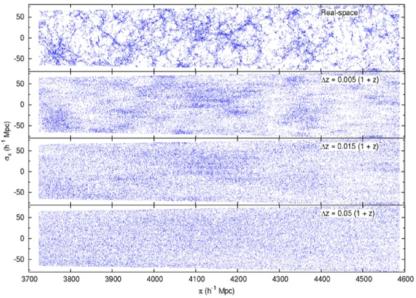
Fig. 1 shows the distribution of haloes in the original catalogue and in the mock photometric catalogues. The Figure shows the real space positions of haloes, not affected by peculiar velocities, and thus does not show the finger-of-God or coherent infall effects observed in spectroscopic surveys. Due to redshift errors, structures which are clearly seen in real space are smoothed and hardly recognizable in photometric redshift data.

Figure 1: The distribution of haloes in the four catalogues used: the original real-space catalogue, and the three mock photometric catalogues. The distribution is shown projected on a longitudinal plane, and only $20$ per cent of the points are shown, for clarity.

3 Method

The most widely used method to measure the correlation function consists in comparing the distribution of points in the data catalogue with a random distribution of points generated in the same volume. To make the comparison, one calculates the number of pairs with separation in the range $[r,r+\mathrm{d}r]$ between points in the data catalogue ($DD(r)$), between points in the random catalogue ($RR(r)$), and between a point in the real catalogue and a point in the random catalogue ($DR(r)$). The estimator used in this work to compute $\xi(r)$ is (Landy & Szalay, 1993):

$$\hat{\xi}(r)=1+\left(\frac{N_{R}}{N_{D}}\right)^{2}\frac{DD(r)}{RR(r)}-2\frac{N_{R}}{N_{D}}\frac{DR(r)}{RR(r)}\,,$$ (1)

where $N_{D}$ is the number of points in the data catalogue, and $N_{R}$ is the number of points in the random catalogue.

However, this method can not be used when the studied catalogue comes from a photometric survey. The large errors in redshift and hence in the line-of-sight positions produce two effects that have to be considered. On one side, these random shifts in position erase correlations between points, and hence $\xi(r)$ measured according to (1) would be much lower than the real $\xi(r)$. On the other side, as the shifts are only in the line-of-sight direction, isotropy of the distribution is lost. Correlation is only lost along the longitudinal direction, but it is conserved in the transverse plane.

The method we used to recover real-space $\xi(r)$ from the mock photometric redshift catalogues is the same described in Davis & Peebles (1983) and Saunders et al. (1992) for spectroscopic surveys. It is based in the decomposition of pair separations in parallel and perpendicular distances ($\pi$ and $\sigma$, respectively).

Let $\mn@boldsymbol{s_{1}}$ and $\mn@boldsymbol{s_{2}}$ be the measured positions (in ‘observed redshift space’) of two points in the catalogue. We then define the separation vector, $\mn@boldsymbol{s}\equiv\mn@boldsymbol{s_{2}}-\mn@boldsymbol{s_{1}}$, and the line-of-sight vector, $\mn@boldsymbol{l}\equiv\mn@boldsymbol{s_{1}}+\mn@boldsymbol{s_{2}}$, of the pair. From these, we now define the parallel and perpendicular distances of the pair as

$$\pi\equiv\frac{|\mn@boldsymbol{s}\cdot\mn@boldsymbol{l}|}{|\mn@boldsymbol{l}|}\quad,\quad\sigma\equiv\sqrt{\mn@boldsymbol{s}\cdot\mn@boldsymbol{s}-\pi^{2}}\,.$$ (2)

Once we have defined $\pi$ and $\sigma$ for each pair of points, we can calculate the two-dimensional correlation function, $\xi(\sigma,\pi)$ in an analogous way to equation (1), substituting the $(r)$ dependence by $(\sigma,\pi)$. From $\xi(\sigma,\pi)$, we define the projected correlation function as

$$\Xi(\sigma)\equiv 2\int_{0}^{\infty}\xi(\sigma,\pi)\mathrm{d}\pi\,.$$ (3)

As $\Xi$ depends only on $\sigma$, and the angle between any pair of points is small, it will not be affected significantly by redshift errors, as these will mainly produce shifts in $\pi$.

Assuming that the real-space distribution is isotropic, we can relate $\Xi$ to the real-space correlation function, $\xi_{r}$, as

$$\Xi(\sigma)=2\int_{\sigma}^{\infty}\xi_{r}(r)\frac{r\mathrm{d}r}{\left(r^{2}-\sigma^{2}\right)^{1/2}}\,.$$ (4)

This relation can be inverted, obtaining $\xi_{r}$ in terms of $\Xi$ as the Abel integral:

$$\xi_{r}(r)=-\frac{1}{\pi}\int_{r}^{\infty}\frac{\mathrm{d}\Xi(\sigma)}{\mathrm{d}\sigma}\frac{\mathrm{d}\sigma}{\left(\sigma^{2}-r^{2}\right)^{1/2}}\,.$$ (5)

Therefore, the method proposed to compute $\xi(r)$ from photometric survey data consists of the following steps. We first obtain $\xi(\sigma,\pi)$ from counting pairs of points in the data and in the random catalogues. The projected correlation function, $\Xi(\sigma)$, is then obtained by integration of equation (3). Finally, the real-space correlation function, $\xi(r)$, is calculated from equation (5). Some problems arise in the numerical integration of equations (3) and (5). Both integrals extend formally to $+\infty$. However, when computing them numerically, we have to set finite upper limits, $\pi_{\rm max}$ and $\sigma_{\rm max}$.

In the first case, the value of $\pi_{\rm max}$ should be large enough to include almost all the correlated pairs. However, if it is too large, this would introduce extra noise in the calculation.

When integrating equation (5), the upper limit $\sigma_{\rm max}$ is fixed, for pencil-beam surveys, by the maximum transverse separation allowed by the geometry. The way we used to evaluate (5) was that of Saunders et al. (1992). We interpolated linearly $\Xi$ between its values in each $\sigma$ bin, and then integrated (5) analytically. Taking $\Xi_{i}$ as the value of $\Xi$ for the bin centred at $\sigma_{i}$, we have

$$\xi(\sigma_{i})=-\frac{1}{\pi}\sum_{j\geq i}\frac{\Xi_{j+1}-\Xi_{j}}{\sigma_{j+1}-\sigma_{j}}\ln\left(\frac{\sigma_{j+1}+\sqrt{\sigma_{j+1}^{2}-\sigma_{i}^{2}}}{\sigma_{j}+\sqrt{\sigma_{j}^{2}-\sigma_{i}^{2}}}\right)\,.$$

Redshift errors will influence the result in two ways. First, these errors change the apparent line-of-sight direction $\mn@boldsymbol{l}/|\mn@boldsymbol{l}|$ (see equation (2)), and through that, the apparent line-of-sight distance $\pi$, and, most important, the perpendicular distance $\sigma$. These errors grow with the redshift error and with the width of the galaxy pair.

Another, and much stronger source of errors is the assumption that the apparent distance in redshift space is the real distance between two galaxies – this assumption is necessary to obtain our basic integral relation (4). In case of photometric errors, this assumption is hardly justified, but we will see that the inverted correlation functions are close to the real one, anyway. The errors caused by this assumption grow with the redshift errors.

4 Results

We tested the deprojection method to measure $\xi(r)$ using the mock photometric catalogues described in Section 2. We applied the method described above to data from the three mock catalogues, and obtained $\xi_{\rm dep}(r)$ in each case. These were then compared to the real-space $\xi_{r}(r)$ calculated from the undistorted simulation catalogue using equation (1) directly.

The value used for the integration limit in equation (5) was $\sigma_{\rm max}=130\,h^{-1}\,\mathrm{Mpc}$. This is about $80$ per cent of the maximum transverse separation allowed by the geometry of the light-cone. We used $32$ bins in $\sigma$, logarithmically spaced between $0.1\,h^{-1}\,\mathrm{Mpc}$ and $\sigma_{\rm max}$.

We performed several tests to choose the appropriate value for $\pi_{\rm max}$, scaling it relative to the $\Delta z$ of the catalogue considered. The $\xi(r)$ recovered increased with $\pi_{max}$ for values $\pi_{\rm max}\la 3\Delta z$, and converged to fixed values for larger $\pi_{\rm max}$. However, the noise also increased with $\pi_{\rm max}$. We adopted a conservative value of $\pi_{\rm max}\simeq 4\Delta z$ for our calculations, in order to be sure to include all correlated pairs, and not introducing too much extra noise.

To estimate the correlation function error and covariance between bins in $r$, we used the jackknife method (see e.g. Zehavi et al., 2005b). We divided our volume in $12$ equal sub-volumes, and constructed our jackknife samples omitting one sub-volume at a time. We repeated the full calculation of $\xi(r)$ for each of these samples. Denoting by $\xi_{i}^{k}$ the value of the correlation function obtained for bin $i$ in jackknife sample $k$, the covariance matrix is then

$$C_{ij}=\frac{N-1}{N}\sum_{k=1}^{N}\left(\xi_{i}^{k}-\bar{\xi_{i}}\right)\left(\xi_{j}^{k}-\bar{\xi_{j}}\right)\,,$$

where $\bar{\xi_{i}}$ is the average of the values obtained for bin $i$, and $N=12$.

4.1 Effect of redshift errors on $\xi(\sigma,\pi)$

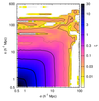
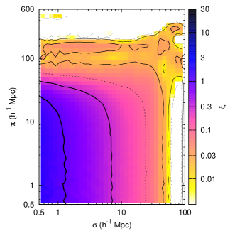
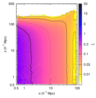
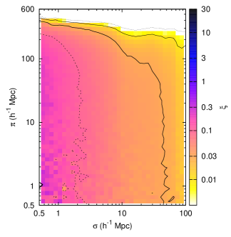
As a first step in the calculation of $\xi(r)$, we calculated $\xi(\sigma,\pi)$ for each mock catalogue. The results are shown in Fig. 2. We also plot the $\xi(\sigma,\pi)$ obtained in the real-space catalogue, for comparison. Two effects of the redshift errors can be observed. First, correlation decreases with the value of $\Delta z$ for each catalogue. Also, there is a loss of symmetry of $\xi(\sigma,\pi)$ in these plots. In real space, due to the isotropy of the distribution, $\xi(\sigma,\pi)$ has circular symmetry (seen as a ‘boxy’ symmetry in the logarithmic scale used). However, we can see that when we calculate it for the mock photometric catalogues, the distribution gets stretched along the $\pi$ axis.

Figure 2: The two-dimensional correlation function $\xi(\sigma,\pi)$ obtained for the real space catalogue (top left), and for the mock photometric catalogues with $\Delta z=0.005(1+z)$ (top right), $\Delta z=0.015(1+z)$ (bottom left) and $\Delta z=0.05(1+z)$ (bottom right). Contours are drawn at $\xi=10,3,1,0.3,0.1,0.03,0.01,0$, with decreasing thickness. Contours at $0.1$ and $0$ are dashed.

4.2 Tests of the deprojection method

When comparing our results for $\xi_{\rm dep}(r)$ with the real-space $\xi_{r}(r)$, we restricted the analysis to the range $r\in[0.5,30]\,h^{-1}\,\mathrm{Mpc}$. The lower limit is given by the way haloes were selected in the simulation. They were selected using a friends-of-friends algorithm, therefore if we had two haloes at a too small separation, they would merge into a single halo (Heinämäki et al., 2005). This prevents us from measuring $\xi(r)$ at such small distances. The upper limit was fixed because of the geometry of the light-cone. As the maximum separation along the short transverse axis is between $30-40\,h^{-1}\,\mathrm{Mpc}$, we can not trust our method beyond these scales.

We measured $\xi_{r}(r)$ directly from the real-space catalogue. In order to compare the real-space result to the one obtained using our method in the mock photometric catalogues, we fitted $\xi_{r}(r)$ by a third-order spline.

From $\xi(\sigma,\pi)$, we obtained the projected correlation function $\Xi(\sigma)$ for each of the mock photometric catalogues. In Fig. 3 we compare the function $\Xi(\sigma)$ calculated for the mock catalogues to the function obtained from the spline fit to the real-space $\xi_{r}(r)$, according to equation (4). The results obtained for the $\Delta z/(1+z)=0.005$ and $\Delta z/(1+z)=0.015$ catalogues follow closely the real-space result. In the case of the $\Delta z/(1+z)=0.05$ catalogue, however, $\Xi(\sigma)$ falls below the real-space result for $r\ga 10\,h^{-1}\,\mathrm{Mpc}$. This feature is due to the fact that the value of $\pi_{\rm max}=600\,h^{-1}\,\mathrm{Mpc}$ used for that catalogue gets close to the line-of-sight length of the simulation box used. As $\pi_{\rm max}$ scales with $\Delta z$, this issue does not affect the other catalogues.

Figure 3: The projected correlation function obtained from the mock photometric catalogues, compared to the real-space result. The solid line corresponds to a spline fit to $\xi_{r}(r)$, as explained in the text. Small shifts have been applied along the $\sigma$ axis, for clarity. The feature observed at large scales for the $\Delta z=0.05(1+z)$ catalogue is due to the large $\pi_{\rm max}$ value used in that case.

Our final result for the deprojected correlation function, $\xi_{\rm dep}(r)$ obtained from the mock photometric catalogues is shown in Fig. 4, where we compare it to the real-space correlation function, $\xi_{r}(r)$.

Figure 4: Comparison between the deprojected correlation function, $\xi_{\rm dep}(r)$ (open circles), and the real-space correlation function, $\xi_{\rm r}(r)$ (solid circles), for each mock photometric catalogue. The error bars plotted correspond to the diagonal terms in the covariance matrix, $C_{ii}^{1/2}$.

To quantify the quality of the recovery, we used an ‘average normalized residual’, $\Delta\xi$, as figure of merit, defined as

$$\Delta\xi=\frac{1}{N}\sum_{i}\left|\frac{\xi_{\rm dep}(r_{i})-\xi_{r}(r_{i})}{\xi_{r}(r_{i})}\right|\,,$$

where $r_{i}$ are the values of the bins in $r$ where we measure $\xi$, and $N$ is the number of such bins considered.

Without prior knowledge of $\xi_{r}(r)$ we could anyhow estimate the quality of the recovery calculating the quantity:

$$\widehat{\Delta\xi}=\frac{1}{N}\sum_{i}\frac{C_{ii}^{1/2}}{\left|\xi_{\rm dep}(r_{i})\right|}\,.$$

We show the values of $\Delta\xi$ and $\widehat{\Delta\xi}$ obtained for the different mock catalogues in Table 1. We computed them for different ranges in $r$, in order to assess the validity of the method at different scales. From the values of $\Delta\xi$ we see that we recover $\xi(r)$ within a $5$ per cent in the average for scales $r<10\,h^{-1}\,\mathrm{Mpc}$ for mock catalogues with $\Delta z\leq 0.015(1+z)$. At larger scales, the deviations from $\xi_{r}$ are larger ($12-20$ per cent). In the case with the largest redshift errors, our method is only valid for very small scales, $r<2\,h^{-1}\,\mathrm{Mpc}$, where the deviations are of a $7$ per cent. We note that, in all cases where the method is valid, $\widehat{\Delta\xi}>\Delta\xi$. Hence, the jackknife method allows us to estimate the errors to an acceptable precision. We remark, however, that for large values of $\Delta z$ the jackknife error underestimates the real one as measured from the residuals or compared to other $\Delta z$ values, specially over medium scales ($2-20\,h^{-1}\,\mathrm{Mpc}$).

Table 1: Values of $\Delta\xi$ and $\widehat{\Delta\xi}$ obtained for the three mock photometric catalogues and for different scale ranges.

	$\frac{\Delta z}{(1+z)}=0.005$		$\frac{\Delta z}{(1+z)}=0.015$		$\frac{\Delta z}{(1+z)}=0.05$
Range ($h^{-1}\,\mathrm{Mpc}$)	$\Delta\xi$	$\widehat{\Delta\xi}$	$\Delta\xi$	$\widehat{\Delta\xi}$	$\Delta\xi$	$\widehat{\Delta\xi}$
$0.5<r<30$	$0.07$	$0.17$	$0.09$	$0.26$	$0.36$	$0.67$
$0.5<r<2$	$0.04$	$0.05$	$0.04$	$0.10$	$0.07$	$0.15$
$2<r<10$	$0.05$	$0.09$	$0.05$	$0.16$	$0.28$	$0.16$
$10<r<30$	$0.12$	$0.40$	$0.20$	$0.57$	$0.79$	$1.89$

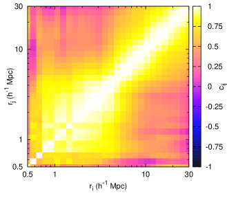
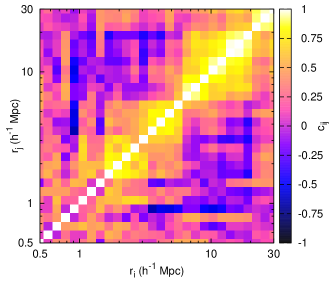
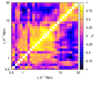
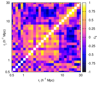
Fig. 5 shows the covariance matrix for the real-space calculation of $\xi_{r}(r)$, and Fig. 6 shows it for the calculation of $\xi_{\rm dep}(r)$ in each case. As the absolute values of the covariance drop rapidly with distance, we show here the normalized covariances

$$c_{ij}=\frac{C_{ij}}{\sqrt{C_{ii}C_{jj}}}.$$

While the absolute values of the covariances grow with the redshift error, and are always larger than the covariances for the real-space correlation function, the structure of the covariance matrix is different. While the real-space covariances are large for almost all bin pairs, the covariance matrices for photometric correlation functions are much closer to diagonal. This is similar to the fact that the best estimates of the correlation function are obtained integrating over line-of-sight distances, even from spectroscopic redshift catalogues (see, e.g., Zehavi et al. (2005a)).

Figure 5: The normalized covariance matrix ($c_{ij}$) of the correlation function measured directly from the real-space catalogue.

Figure 6: The normalized covariance matrices ($c_{ij}$) of the deprojected correlation function measured directly from the mock photometric catalogues with $\Delta z=0.005(1+z)$ (top left), $\Delta z=0.015(1+z)$ (top right) and $\Delta z=0.05(1+z)$ (bottom).

In order to assess the robustness of the method to the presence of ‘catastrophic’ redshift determinations, we repeated the calculation in catalogues containing 5 per cent of such outliers. Outliers were created selecting points at random in the original catalogue, and assigning them a random distance within the range considered. Even with the conservative assumption of a large fraction of outliers, our method recovers $\xi(r)$, although the values of $\Delta\xi$ are slightly larger in this case, ranging from 5 to 13 per cent for $r<10\,h^{-1}\,\mathrm{Mpc}$ and $\Delta z\leq 0.015(1+z)$. The result obtained for the catalogue with $\Delta z=0.015(1+z)$, and containing 5 per cent of outliers is shown in Fig. 7. Similar results were obtained when a fraction of the outliers were taken from a Poisson sample within our volume. This case would reproduce the effect of stellar contamination in the catalogue.

Figure 7: The deprojected correlation function obtained for the $\Delta z=0.015(1+z)$ catalogue with and without outliers. The continuous line is the real-space correlation function.

We performed an additional test of the deprojection method using a realization of a segment Cox process, for which an analytical expression of the correlation function is known (Martinez et al., 1998). The results of those tests are further explained in Appendix A.

5 Conclusions

We have shown the reliability of recovering the real-space two-point correlation function from photometric redshift surveys. We have used light-cone simulations to produce mock catalogues that have been distorted by randomizing along the line of sight the object positions following Gaussian distributions with different variances similar to the associated nominal errors of the photometric redshift surveys $\Delta z/(1+z)$.

The method used to recover the real-space correlation function consists in obtaining the projected correlation function by integrating the two-dimensional correlation function along the line of sight. The projected correlation function is then deprojected assuming that redshift errors do not affect transverse distances.

The deprojection method applied on the distorted mock surveys provides quite satisfactory results for recovering the real-space correlation function. We have quantified the quality of the recovering process as a function of the errors in the photometric redshifts. Our method was able to recover the real-space correlation function within a $5$ per cent for $r<10\,h^{-1}\,\mathrm{Mpc}$ from photometric catalogues with $\Delta z\leq 0.015(1+z)$. For larger redshift errors, the method is only valid (within a $7$ per cent) for smaller scales, $r<2\,h^{-1}\,\mathrm{Mpc}$. Hence, our method allows the extraction of useful information on the clustering of galaxies through the correlation function. That information can be used for the estimation of cosmological parameters based on data from photometric redshift surveys.

We discuss now possible alternatives to the method exposed here. A variation of the method would be to use a smaller value of $\pi_{\rm max}$ in the integration of equation (3), and multiply the result by a constant correction factor. This would reduce the extra noise introduced by the integration along a large range in the $\pi$ direction. We found that, for $\pi_{\rm max}\simeq\Delta z$, a correction factor of $\simeq 2$ works well in our simulation, generally reducing the error. However, the optimal value is slightly different for each mock photometric catalogue. The main problem for the use of this method would be the accurate determination of the correction factor in each case, as any deviation from the optimal value would introduce a bias in the result. The Gaussian approximation used here is probably not so close to reality as to infer that constant from our simulations.

Another possible alternative to the method described in this work could make use of the new estimator $\omega$ presented in Padmanabhan, White & Eisenstein (2007). They proposed $\omega$ as an alternative to the projected correlation function to use with spectroscopic survey data. In principle, it can also be applied to photometric redshift survey data, in a way similar to the one presented here, but we did not investigate further this possibility.

Appendix A Test of the method using a segment Cox process

In order to test our method against an analytical prediction for $\xi(r)$, we used a distribution of points given by a segment Cox process. This process is produced in the following way (Martínez & Saar, 2002): segments of a given length, $l$, are randomly scattered within a volume. Then, points are randomly distributed along these segments. The lenght density of the system of segments is $L_{V}=\lambda_{s}l$, where $\lambda_{s}$ is the mean number of segments per unit volume. The density of the point process is then

$$\lambda=\lambda_{l}L_{V}=\lambda_{l}\lambda_{s}l\,,$$

where $\lambda_{l}$ is the mean number of points per unit length of the segments. The correlation function of the point process equals the correlation function of the system of segments (Stoyan, Kendall & Mecke, 1995), which is given by

$$\xi_{\rm Cox}(r)=\left\{\begin{array}[]{ll}\frac{1}{2\pi r^{2}L_{V}}-\frac{1}{2\pi rlL_{V}}\,,&r\leq l\\ 0\,,&r>l\end{array}\right.\,.$$ (6)

We simulated a segment Cox process in the same volume considered in the rest of this work. The parameters we used were $l=50\,h^{-1}\,\mathrm{Mpc}$, $\lambda_{s}=2\cdot 10^{-4}\,h^{3}\,\mathrm{Mpc}^{-3}$ and $\lambda_{l}=4\,h\,\mathrm{Mpc}^{-1}$, which result in $L_{V}=0.01\,h^{2}\,\mathrm{Mpc}^{-2}$ and $\lambda=0.04\,h^{3}\,\mathrm{Mpc}^{-3}$. These parameters were chosen to approximately match the density of points and the behaviour of $\xi(r)$ in the haloes simulation. We considered the catalogue obtained directly from the segment Cox process as the ‘real-space’ catalogue. We created three mock ‘photometric redshift catalogues’ following the same procedure and using the same values for $\Delta z$ as described in Section 2 .

Figure 8: The correlation function measured in the real-space and the three mock ‘photometric’ catalogues obtained from a segment Cox process (open circles), compared to the analytical prediction, equation (6), for this process (solid line).

We calculated directly the correlation function for the real-space catalogue according to equation (1). For the three mock ‘photometric catalogues’, we used the method described in Section 3 to obtain the deprojected correlation function. The estimation of errors was performed using the same jackknife method as described above for the haloes simulation case. We checked that the errors obtained were comparable to the variance of the results from several realizations of the Cox process. The comparison of our results to the analytical prediction (6) is shown in Fig. 8.

We quantify the quality of the recovery in the same way as we did for the haloes simulation, using the quantities $\Delta\xi$ and $\widehat{\Delta\xi}$. In this case, we define $\Delta\xi$ as the relative deviation of $\xi_{\rm dep}(r)$ from the analytical prediction $\xi_{\rm Cox}(r)$ (equation (6)). The values obtained are shown in Table 2.

Table 2: Values of $\Delta\xi$ and $\widehat{\Delta\xi}$ obtained for the three mock photometric catalogues obtained from a Cox process, and for different scale ranges.

	$\frac{\Delta z}{(1+z)}=0.005$		$\frac{\Delta z}{(1+z)}=0.015$		$\frac{\Delta z}{(1+z)}=0.05$
Range ($h^{-1}\,\mathrm{Mpc}$)	$\Delta\xi$	$\widehat{\Delta\xi}$	$\Delta\xi$	$\widehat{\Delta\xi}$	$\Delta\xi$	$\widehat{\Delta\xi}$
$0.5<r<10$	$0.08$	$0.16$	$0.18$	$0.23$	$0.35$	$0.40$
$0.5<r<2$	$0.06$	$0.08$	$0.07$	$0.12$	$0.23$	$0.21$
$2<r<10$	$0.10$	$0.22$	$0.27$	$0.33$	$0.46$	$0.57$

We recover the real-space correlation function within a $10$ per cent for the $\Delta z/(1+z)=0.005$ catalogue. In this case, however, our method starts to fail at $r\simeq 3-4\,h^{-1}\,\mathrm{Mpc}$ for the $\Delta z/(1+z)=0.015$ catalogue (this is seen as a larger value of $\Delta\xi$ for this range, and as an increasing trend in Fig. 8). When applying the method to the $\Delta z/(1+z)=0.05$ catalogue, $\xi_{\rm dep}(r)$ is consistently higher than $\xi_{\rm Cox}(r)$. Although this bias could be an artefact of this particular point process, it also means that the deprojection method described in this work can not be fully trusted when it is applied to catalogues with large redshift errors.

References

- Baum (1962) Baum W. A., 1962, in McVittie G. C., ed., Problems of Extra-Galactic Research Vol. 15 of IAU Symposium, Photoelectric Magnitudes and Red-Shifts. pp 390–+
- Benítez (2000) Benítez N., 2000, ApJ, 536, 571
- Benítez et al. (2008) Benítez N., et al., 2008, ApJ, in press (arXiv:0807.0535)
- Blake & Bridle (2005) Blake C., Bridle S., 2005, MNRAS, 363, 1329
- Coe et al. (2006) Coe D., Benítez N., Sánchez S. F., Jee M., Bouwens R., Ford H., 2006, AJ, 132, 926
- Connolly et al. (1995) Connolly A. J., Csabai I., Szalay A. S., Koo D. C., Kron R. G., Munn J. A., 1995, AJ, 110, 2655
- Davis & Peebles (1983) Davis M., Peebles P. J. E., 1983, ApJ, 267, 465
- Fernández-Soto et al. (2008) Fernández-Soto A., et al., 2008, Il Nuovo Cimento, in press (arXiv:0805.3319)
- Fernández-Soto et al. (2002) Fernández-Soto A., Lanzetta K. M., Chen H.-W., Levine B., Yahata N., 2002, MNRAS, 330, 889
- Fernández-Soto et al. (2001) Fernández-Soto A., Lanzetta K. M., Chen H.-W., Pascarelle S. M., Yahata N., 2001, ApJS, 135, 41
- Hawkins et al. (2003) Hawkins E., et al., 2003, MNRAS, 346, 78
- Heinämäki et al. (2005) Heinämäki P., Suhhonenko I., Saar E., Einasto M., Einasto J., Virtanen H., 2005, preprint (arXiv:astro-ph/0507197)
- Ilbert et al. (2008) Ilbert O., et al., 2008, ApJ, in press (arXiv:0809.2101)
- Koo (1986) Koo D. C., 1986, in Chiosi C., Renzini A., eds, Spectral Evolution of Galaxies Vol. 122 of Astrophysics and Space Science Library, Quests for primeval galaxies - A review of optical surveys. pp 419–438
- Landy & Szalay (1993) Landy S. D., Szalay A. S., 1993, ApJ, 412, 64
- Madgwick et al. (2003) Madgwick D. S., et al., 2003, MNRAS, 344, 847
- Martinez et al. (1998) Martinez V. J., Pons-Borderia M.-J., Moyeed R. A., Graham M. J., 1998, MNRAS, 298, 1212
- Martínez & Saar (2002) Martínez V. J., Saar E., 2002, Statistics of the Galaxy Distribution. Chapman & Hall/CRC, Boca Raton, FL
- Moles et al. (2006) Moles M., et al., 2006, in del Toro Iniesta J. C., Alfaro E. J., Gorgas J. G., Salvador-Solé E., Butcher H., eds, The Many Scales in the Universe: JENAM 2004 Astrophysics Reviews Springer, Dordrecht
- Moles et al. (2008) Moles M., et al., 2008, AJ, 136, 1325
- Padmanabhan et al. (2007) Padmanabhan N., White M., Eisenstein D. J., 2007, MNRAS, 376, 1702
- Phleps et al. (2006) Phleps S., Peacock J. A., Meisenheimer K., Wolf C., 2006, A&A, 457, 145
- Saunders et al. (1992) Saunders W., Rowan-Robinson M., Lawrence A., 1992, MNRAS, 258, 134
- Stoyan et al. (1995) Stoyan D., Kendall W. S., Mecke J., 1995, Stochastic Geometry and its Applications. John Wiley & Sons, Chischester, England
- Wolf et al. (2003) Wolf C., Meisenheimer K., Rix H.-W., Borch A., Dye S., Kleinheinrich M., 2003, A&A, 401, 73
- Zehavi et al. (2004) Zehavi I., et al., 2004, ApJ, 608, 16
- Zehavi et al. (2005a) Zehavi I., et al., 2005a, ApJ, 621, 22
- Zehavi et al. (2005b) Zehavi I., et al., 2005b, ApJ, 630, 1