Coherent detection method of gravitational wave bursts for spherical antennas

Abstract

We provide a comprehensive theoretical framework and a quantitative test of the method we recently proposed for processing data from a spherical detector with five or six transducers. Our algorithm is a trigger event generator performing a coherent analysis of the sphere channels. In order to test our pipeline we first built a detailed numerical model of the detector, including deviations from the ideal case such as quadrupole modes splitting, and non-identical transducer readout chains. This model, coupled with a Gaussian noise generator, has then been used to produce six time series, corresponding to the outputs of the six transducers attached to the sphere. We finally injected gravitational wave burst signals into the data stream, as well as bursts of non-gravitational origin in order to mimic the presence of non-Gaussian noise, and then processed the mock data. We report quantitative results for the detection efficiency versus false alarm rate and for the affordability of the reconstruction of the direction of arrival. In particular, the combination of the two direction reconstruction methods can reduce by a factor of 10 the number false alarms due to the non-Gaussian noise.

I Introduction

Started more than forty years ago with the pioneering work of Weber Weber , the rush for direct gravitational wave (GW) detection have nowadays reached a crucial phase. On one side, the era of large interferometers (LIGO, VIRGO, GEO, TAMA) intf_web has begun and the next, so-called “advanced” versions of the interferometers are currently considered as the most likely candidate to make the first detection (although uncertainties in stellar population estimates still do not allow to keep this goal for granted, see deFreitasPacheco:2006bh ).

On the other side, resonant bars bar_web like the INFN ones (EXPLORER, NAUTILUS, AURIGA) or ALLEGRO seem to have exhausted their original leading role after several years of impressive performances (see for instance Astone:2006ut for some reports on the most recent runs) which made them by far the best instruments for a long time.

This does not mean at all that resonant detectors are going to be out of business, as resonant bars are currently running as a network Astone:2007vu and joint analyses with interferometers have already taken place Collaboration:2007paa (and are foreseen in the future). Moreover high-performance, new generation antennas (like large spheres Fafone:2006nr or dual detectors Bonaldi:2003at ) have already been conceived. In this framework, the two small spherical detectors in Leiden Gottardi:2007zn and San Paulo Aguiar:2006va , that are already in the commissioning phase, can rightfully be considered as the first specimens of this new generation.

What makes a sphere really different from bars and interferometers is the fact of being a multichannel detector. This distinguishing feature not only determines its isotropic sensitivity and its capability to reconstruct the GW direction, but also opens the way to new opportunities, and issues, from the data analysis point of view. After the seminal work of Wagoner and Paik Wagoner , where the basic features of the detector have been pointed out, more and more detailed sphere models and configurations have been studied by several authors Zhou:1995en ; Coccia:1995yi ; Lobo:1996ae ; Stevenson:1996rw ; Merkowitz:1997qc ; Merkowitz:1997qs ; Lobo:2000hy ; Gasparini:2006vb ; Gottardi:2006gn . In particular, various solutions have been proposed to the problems of the ideal transducers configuration Lobo:2000hy , parameter reconstruction Merkowitz:1997qs ; Zhou:1995en , and multidimensional data analysis Stevenson:1996rw .

The analysis method that we have set up and studied in the present work is the result of a synthesis and a refinement of some of these contributions, and is intended to represent the core of the pipeline that we are building for the miniGRAIL detector. Some preliminary results have already been proposed in Foffa:2008pm , here we expose the theoretical foundations and assess quantitatively the solidity of the method as an event trigger-generator.

Particular care has been dedicated to all those concrete details that enter the game as “theoretical” data analysis is turned into a real, working device: these include, in primis, attention to the problem of false detections and keeping under control the computation time required by the pipeline.

The first part of the paper is devoted to building an accurate detector model and to the generation of a set of simulated data, expanding the treatment in Foffa:2008pm . We consider a real, imperfect sphere with six read-out electromechanical amplificators of its surface oscillations. Our method works also with five outputs, while using a smaller number of transducers significantly degrade the performances of the detector, even if four transducers are in principle sufficient to fully reconstruct the GW tensor.

After having written the basic equations, we work out the spectrum of each transducer’s output and we generate simulated data starting from the elementary noises which enter the detector at different levels. Then we discuss the problem of extracting the GW parameters out of the data.

In the second part we describe the method to generate triggers of events, based on the coherent WaveBurst algorithm, the event trigger generator used by the LIGO-VIRGO burst data analysis group. We adapted it to a multimode detector, where different channels have correlated noise, differently from the LIGO-VIRGO situation where the detectors are not co-located. The availability of several channels allows a determinaton of the arrival direction of the burst through a standard likelihood analysis method. Such a determination is then validated by a consistency check with the geometrical method exposed in paragraph III.3, named determinant method, which provides an independent indication of the arrival direction.

In the last section the efficiency of the method for four different amplitudes of injected bursts is shown. We tested the method against injections of both GW and non-GW signals, where for non-GW signals the injection amplitude is shared randomly the five quadrupolar channels.

While each of the two above-mentioned method alone is not able to distinguish between GW and non-GW excitations, we find that the combination ot the two allows to reduce the false alarm rate by roughly one order of magnitude, while keeping a good detection efficiency, and provides a good determination of the arrival direction of the signal. The multi-mode coherent analysis is thus able to compute all the relevant parameters of a GW and to reduce the false alarm rate.

II Model of the detector

II.1 Equations for modes, transducers and readout currents

The sphere is well modeled as a set of coupled oscillators, which describe the dynamics of the relevant sphere vibrational modes, of the transducers, and of the electrical circuit that are at the core of the readout devices. As the relevant equations have been already discussed in detail by several authors (see for instance Merkowitz:1997qc ; Gottardi:2006gn ; Maggiore:1900zz ), we jump to the mathematical core of the problem, skipping introductory material and definitions that can be found in the literature. These equations hold for any number of sphere modes and transducers, although in the following subsections we will specify our choices for such numbers. For the sake of clarity and completeness, the definitions and values of all the quantities appearing below are summarized in fig.1 and in Appendix A.

Figure 1: The readout scheme, from Foffa:2008pm .

In Fourier space, the amplitudes $\xi_{N}$ of the various radial modes of the sphere obey to the following equations

$$\begin{array}[]{rl}\displaystyle\!\!\!\!\!\!\!\!\!\!\!\!\left(\omega_{N}^{2}-\omega^{2}+i\frac{\omega_{N}\omega}{Q_{N}}\right)\xi_{N}-\alpha_{N}\sum_{k}B_{Nk}\left[\left(\omega_{k}^{2}+i\frac{\omega_{k}\omega}{Q_{k}}\right)\frac{m_{k}}{M}q_{k}-i\frac{E_{k}}{M\omega}J_{k}\right]&=\\ \displaystyle\!\!\!\!\!\!\!\!\!\!\!\!f_{N}-\alpha_{N}\sum_{k}B_{Nk}\frac{m_{k}}{M}f^{t}_{k}&.\end{array}$$ (3)

which relate their dynamics to that of the transducer displacements $q_{k}$ and of the primary currents $J_{k}$ through the position matrix $B_{Nk}\equiv Y_{N}(\theta_{k},\phi_{k})$. The equations for the transducer displacements are:

$$-\omega^{2}\sum_{N}B_{kN}\alpha_{N}\xi_{N}+\left(\omega_{k}^{2}-\omega^{2}+i\frac{\omega_{k}\omega}{Q_{k}}\right)q_{k}-i\frac{E_{k}}{m_{k}\omega}J_{k}=f^{t}_{k}\,,$$ (4)

while the readout circuit can be described through the equations driving the primary currents and the secondary ones, $I_{k}$, which are proportional to the actual outputs of the detector:

$$E_{k}q_{k}+\left[r_{k}+i\left(\omega L^{p}_{k}-\frac{1}{\omega C_{k}}\right)\right]J_{k}-i\omega M^{ps}_{k}(I_{k}-f^{i}_{k})=f^{p}_{k}\,,$$ (5)

$$-i\omega M^{ps}_{k}J_{k}+i\omega\left(L^{s}_{k}+L^{i}_{k}\right)(I_{k}-f^{i}_{k})=f^{s}_{k}\,.$$ (6)

The $f$’s appearing above are the stochastic forces related to the various dissipative components of the detector; their action can be described through the corresponding noise spectral densities:

$$<f_{x}(\omega)f^{*}_{y}(\omega^{\prime})>\equiv S_{xy}(\omega)\delta(\omega-\omega^{\prime})\,.$$ (7)

The non-vanishing components of the noise spectral density matrix are:

$$S_{NN^{\prime}}=2k_{B}T\frac{\omega_{N}}{MQ_{N}}\delta_{NN^{\prime}}\,,\quad\!S^{t}_{kk^{\prime}}=2k_{B}T\frac{\omega_{k}}{Q_{k}m_{k}}\delta_{kk^{\prime}}\,,\quad\!S^{p}_{kk^{\prime}}=2k_{B}Tr_{k}\delta_{kk^{\prime}}\,,$$ (8)

and, according to the Clarke model Clarke for the SQUID,

$$S^{s}_{kk^{\prime}} = 16\frac{k_{B}T}{R^{sh}_{k}}\left(\frac{L^{SQ}_{k}}{M^{SQ}_{k}}\right)^{2}\delta_{kk^{\prime}}\,,$$

$$S^{i}_{kk^{\prime}}(\omega) = 11\omega^{2}\frac{k_{B}T}{R^{sh}_{k}}(M^{SQ}_{k})^{2}\delta_{kk^{\prime}}\,,$$ (9)

$$S^{s,i}_{kk^{\prime}}(\omega) = -12i\omega\frac{k_{B}T}{R^{sh}_{k}}L^{SQ}_{k}\delta_{kk^{\prime}}\,,$$

where $S_{NN^{\prime}},S_{kk^{\prime}}^{t},S^{p}_{kk^{\prime}},S^{s}_{kk^{\prime}},S_{kk^{\prime}}^{i},S^{s,i}_{kk^{\prime}}$ are the spectral densities of, respectivley: the forces acting on the the radial mode displacements, on the transducers, on the primary currents, on the secondary currents, the spectral densities of the secondary current noises and the spectral density of the secondary current noise forces times the secondary current noise.

II.2 Output current determination and simulation

II.2.1 Specification of the system

By using the following matrix notation

$$\displaystyle{\cal Z}\equiv$$

$$\displaystyle\!\!\!\!\!\!\!\!\!\!\!\!\!\!\!\!\!\!\!\!\!\!\!\!\!\!\!\!\!\!\!\!\!\left(\begin{array}[]{c|c|c|c}{\cal D}\left[\Omega_{N}\right]&-{\cal D}\left[\alpha_{N}\right]\cdot{\cal B}_{Nk}\cdot{\cal D}\left[\tilde{\Omega}_{k}\right]&{\cal D}\left[\alpha_{N}\right]\cdot{\cal B}_{Nk}\cdot{\cal D}\left[\varepsilon_{k}/m_{k}\right]&0\\ \hline\cr-\omega^{2}{\cal B}^{T}_{kN}\cdot{\cal D}\left[\alpha_{N}\right]&{\cal D}\left[\Omega_{k}\right]&-{\cal D}\left[\varepsilon_{k}/M\right]&0\\ \hline\cr 0&{\cal D}\left[E_{k}\right]&{\cal D}\left[RLC_{k}\right]&{\cal D}\left[M^{ps}_{k}\right]\\ \hline\cr 0&0&{\cal D}\left[M^{ps}_{k}\right]&{\cal D}\left[{\cal L}^{si}_{k}\right]\end{array}\right)\,,$$ (14)

$${\cal A}\equiv\left(\begin{array}[]{c|c|c|c}{\cal I}_{N}&-{\cal D}\left[\alpha_{N}\right]\cdot{\cal B}_{Nk}\cdot{\cal D}\left[m_{k}/M\right]&0&0\\ \hline\cr 0&{\cal I}_{k}&0&0\\ \hline\cr 0&0&{\cal I}_{k}&0\\ \hline\cr 0&0&0&{\cal I}_{k}\end{array}\right)\,,$$ (19)

$${\cal Q}\equiv\{\xi_{N},q_{k},J_{k},I_{k}-f^{I}_{k}\}\,,\quad{\cal F}\equiv\{f_{N},f^{t}_{k},f^{p}_{k},f^{s}_{k}\}\,,$$ (20)

where ${\cal I}_{n}$ is the $n$-dimensional identity matrix, the dynamical system of equations can be written in a concise way

$${\cal Z}\cdot{\cal Q}={\cal A}\cdot{\cal F}\,,$$ (21)

which in turn implies

$$\{\xi_{N},q_{k},J_{k},I_{k}\}={\cal Z}^{-1}\cdot{\cal A}\cdot{\cal F}+\{0,0,0,f^{I}_{k}\}\,.$$ (22)

This reduces the problem of finding the currents $I_{k}$, and their spectral correlation matrices, to the inversion of the matrix ${\cal Z}$.

In some particular case, such inversion is very easy to compute. For instance, for the case of 6 transducers in the TIGA configuration, if we include in the model only the first 5 quadrupolar sphere modes and the scalar one, then

$$B_{Nk}\cdot B^{T}_{kN}=B^{T}_{kN}\cdot B_{Nk}=\frac{3}{2\pi}{\cal I}_{6}\,.$$ (23)

In this case, in the idealized hypothesis that all the 6 transducers and readout chains are identical, thus implying that all the blocks of the kind ${\cal D}\left[X_{k}\right]$ appearing in ${\cal Z}$ are proportional to the identity, one obtains that the following redefinition

$${\cal Q}\equiv{\cal R}\cdot{\cal Q}^{\prime}\,,$$ (24)

with

$${\cal R}\equiv\left(\begin{array}[]{c|c|c|c}{\cal I}_{N}&0&0&0\\ \hline\cr 0&B_{Nk}&0&0\\ \hline\cr 0&0&B_{Nk}&0\\ \hline\cr 0&0&0&B_{Nk}\end{array}\right)\,,$$ (29)

leads to

$${\cal Z}\cdot{\cal Q}={\cal R}\cdot{\cal Z}^{\prime}\cdot{\cal Q}^{\prime}\,,$$ (30)

where all the 16, $6\times 6$ blocks of ${\cal Z}^{\prime}$ are diagonal.

Since ${\cal R}$ is easily invertible by means of eq.(23), the $I_{k}$’s are easily found. This particular case is nothing but a rephrasing of the idea of mode channels of an ideal TIGA configuration, see Merkowitz:1997qc .

However, since our purpose is to simulate a realistic detector, we will not take advantage of any idealization, and we will invert the ${\cal Z}$ matrix numerically.

For the same reason we have decided to include many sphere modes in our model, contrarily to the common practice of considering only the lowest quadrupole multiplet, that is the one that interacts with the GW. More precisely, we have included in our model all the radial modes with resonant frequency below that of the scalar mode: this gives a total of 30 degrees of freedom in this part of the system, distributed among one scalar, one vector, two quadrupolar, one l=3 and one l=4 multiplets. The precise reason of this choice will be discussed in subsection II.3; for the moment we just mention that even if the extra modes resonate far away the interesting region of the spectrum (which is around $3$kHz), nevertheless their inclusion in the model affects the response function even in the relevant spectral region, shifting the peaks in the response function of a few Hz’s, as can be seen in fig.2. In a real detector, however, such shift may be masked by the action of the suspension system, finite-size effects of the transducers and/or some other unmodelled factors. At the moment we are not able to predict the magnitude of these unmodelled effects for miniGRAIL.

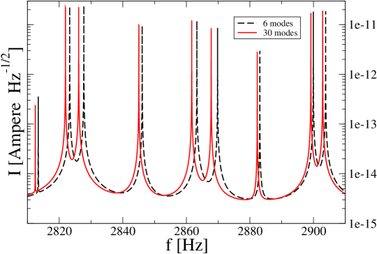
Figure 2: Theoretical output of one of the transducers when 6 or 30 sphere vibrational modes are included in the model. To emphasize the differencies, a restricted region of the spectrum have been displayed: this is the reason why only nine out of the eleven resonant modes are visible.

For what concerns the transducers arrangement, we will stick to the TIGA configuration (with non identical transducers, however), although our analysis can easily be adapted to other configurations, provided the number of transducers is kept equal to six.

II.2.2 From expectation values to a typical noise realization

Once ${\cal Z}$ has been numerically inverted, we can proceed to determine the currents $I_{k}$ through eq.(22), and in particular we can estimate the corresponding spectral density matrix from eqns.(8)-(II.1):

$$<I_{k}(\omega)I^{*}_{k^{\prime}}(\omega^{\prime})>\equiv S^{I}_{kk^{\prime}}(\omega)\delta(\omega-\omega^{\prime})\,.$$ (31)

The square root of one of the diagonal elements of $S^{I}_{kk^{\prime}}$ is shown in fig.4, along with the different noise contributions.

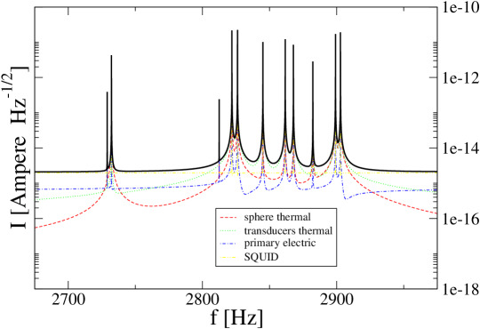
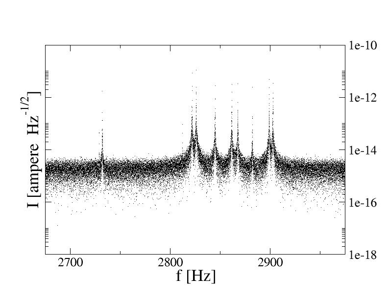
Figure 3: The calculated output of the transducer #0, along with the various noise contributions.

Figure 4: Simulated output of transducer #0, from Foffa:2008pm .

This is still not enough for our purposes: what we really want to get at this stage is not just expectation values and cross-correlations, but an actual realization of a possible detector output. To obtain this, we have generated several time series of white noise, we have taken their numerical Fourier transforms, and ”colored” them according to the spectral dependencies of eqns.(8)-(II.1), thus obtaining a possible realization of the Fourier transform of the various stochastic forces $f$’s. Finally, we have derived, still in Fourier space, the realizations of the currents $I_{k}$, by means of eq.(22), satisfying eq.(31); one result of this procedure is displayed in fig.4.

We underline the fact that fig.4 does not represent just a white spectrum ”colored” according to the expectation value shown in fig.4, but it rather contains, in virtue of the procedure we have adopted to generate it, all the correct cross-correlations with the other output currents, i.e. the non-diagonal elements of eq.(31). This fact is crucial if the injected signals are to be reconstructed.

To summarize the results of this subsection, we have numerically generated the six current outputs of a realistic sphere working in the TIGA configuration. Our model is realistic in the sense that we have chosen the values of all the components of the simulated detector according to what is actually being implemented on miniGRAIL, and we have included an adequate number of sphere vibrational modes.

II.3 Interaction with the GW: the transfer matrix

We now change point of view: we assume that the six secondary currents are given and we would like to determine the sensitivity of our detector to GW’s. In other words, we are trying to reproduce as faithfully as possible a real experimental situation.

We remind that when a GW impinges the detector, a deterministic force is added to the quadrupolar components of $f_{N}$:

$$f_{N}\rightarrow f_{N}+\frac{1}{2}R\chi\ddot{h}_{N}\quad{\rm for}\quad N=0,\dots,4\,,$$ (32)

where $R$ is the sphere radius, $\chi=-0.3278$ for CuAl6% (the alloy miniGRAIL is made of) and the $h_{N}$’s are the quadrupolar spheroidal components of the GW, defined as follows through decomposition via the tensor spherical harmonics:

$$h_{ij}=\sum_{N=0,4}{\cal Y}^{(2)}_{m_{N},ij}h_{N}\,,$$ (33)

with $m_{N}=0,1c,1s,2c,2s$ and $Y^{(2)}_{m_{N}}=\sum_{i,j}{\cal Y}^{(2)}_{m_{N},ij}n^{i}n^{j}$, being $n^{i}$ the versor of the arrival direction of the wave.

II.3.1 Issues in getting the $h_{N}$’s from the transducer outputs

The problem is clearly to get the most possible information about the $h_{N}$’s from the knowledge of the six $I_{k}$’s. For this goal, it would be enough to determine, and most of all to invert somehow, the ${\cal T}_{kN}$ matrix, which is defined as the $k\times 5$ block determined by crossing the last $k$ lines with the first $5$ columns of the matrix ${\cal Z}^{-1}{\cal A}$ which appears in eq.(22). Basically, ${\cal T}_{kN}$ is the matrix entering the relation:

$$I_{k}={\cal T}_{kN}\cdot f_{N}\,.$$ (34)

with $f_{N}$ given by eq.(32), which holds in the limit of very large SNR.

In general, the solution to this problem is very much dependent on the number of transducers. If such number is less than four, then there are not enough experimental inputs to determine all the $h_{N}$’s, and thus the matrix $h_{ij}$ cannot be completely reconstructed. Rather, only some linear combinations of the $h_{N}$’s (or, in another notation, of the GW polarization components) can be determined.

If there are four transducers, then in principle the metric perturbation can be reconstructed, provided one imposes a priori on the data the constraint that the five $h_{N}$’s should form a transverse tensor. The five transducers case is similar, with the advantage that one can use the transversality condition as a veto, thus reducing the false alarm rate at a given SNR, rather then imposing it from the beginning.

If the transducers are six, as in the present case, the situation is more involved because the system is over-constrained by the fact that the $5$ $h_{M}$’s are to be determined by the $6$ outputs. This kind of problem has generally no solution, as it is physically correct since the $I_{k}$’s are not determined only by the GW, but also by the detector noise; however in some cases an optimal solution can be found.

First of all, we have seen that in an ideal TIGA configuration (identical readout chains) a change of basis brings the matrix ${\cal Z}^{\prime}$ to a block diagonal form. By inspection of the form of the system of equations (21) it can be seen that this implies also that the ${\cal T}_{kN}$ matrix has the following pseudo-diagonal form:

$${\cal T}_{kN}\equiv\left(\begin{array}[]{ccccc}*&0&0&0&0\\ 0&*&0&0&0\\ 0&0&*&0&0\\ 0&0&0&*&0\\ 0&0&0&0&*\\ 0&0&0&0&0\end{array}\right)\,,$$ (41)

the last row of zeroes meaning that the sixth redefined component of $I^{\prime}_{k}$ is independent of the $h_{N}$’s. In this case one has just to consider the square, and invertible, matrix made of the first $5$ lines of ${\cal T}_{kN}$: i.e. only the first five $I^{\prime}_{k}$’s (which are nothing else but the TIGA mode channels) are used to find the five $h_{N}$’s and the system is again well determined.

When the idealized conditions for a perfect TIGA configuration no longer hold, the situation becomes more complicated because there is no simple way to get to the form (41) for the ${\cal T}_{kN}$ matrix; in particular, in the general case all the six current outputs (or any linear combination of them) depend on the GW parameters.

In this case, the system (34) is really over-constrained and has in general no exact solution; in such cases, the best one can do from the mathematical point of view is to find the best possible approximate solution for the system, that is, in the case at hand, a vector $f^{*}_{N}$ such that the norm of the vector

$$I_{k}-{\cal T}_{kN}\cdot f^{*}_{N}\,,$$ (42)

is minimal. If the matrix ${\cal T}_{kN}$ has maximum rank, then the pseudo solution $f^{*}_{N}$ can be shown to be unique, and to be given by

$$f^{*}_{N}=({\cal T}^{T}_{Nk}\cdot{\cal T}_{kN})^{-1}\cdot{\cal T}^{T}_{Nk}\cdot I_{k}\,.$$ (43)

This strategy, which has been proposed for example in Merkowitz:1997qs is certainly a good one in the case of very high SNR, while at low SNR, and in particular in the determination of the detector’s sensitivity (where $SNR=1$ by definition), it shows some drawbacks.

The problem is that, when the noise gives a non negligible contribution to the output currents, there is no physical reason to expect that the actual $h_{N}$’s are the ones that minimize the norm of the vector (42).

II.3.2 Inclusion of the scalar mode

Our proposal in this case is to include the scalar vibrational mode of the sphere, so that eqns.(32), (33) are now turned into

$$f_{N}\rightarrow f_{N}+\frac{1}{2}R\chi_{N}\omega^{2}h_{N}\quad{\rm for}\quad N=0,\dots,5\,,$$ (44)

$$h_{ij}=\sum_{N=0,4}{\cal Y}^{(2)}_{m_{N},ij}h_{N}+\frac{{\cal I}_{ij}}{\sqrt{4\pi}}h_{5}\,,$$ (45)

being ${\cal I}_{ij}$ the identity matrix, and $\chi_{N}=\chi$ for $N=0,\dots,4$, while it can be shown that $\chi_{5}=-3.8$.

As we have already discussed, inclusion of the scalar mode makes the position matrix $B_{Nk}$ invertible and orthogonal, see eq.(23), because the row corresponding to the scalar mode is orthogonal to the $5$ lines related to the quadrupolar modes. This means that adding the scalar mode is the best possible way to complete the $5$ quadrupole position vectors to a basis of the six-dimensional linear space.

If we proceed this way, another sixth column must be included in the definition of ${\cal T}_{Nk}$, which now becomes an invertible $6\times 6$ matrix. In other words, including the scalar mode is a way to turn an over-constrained rectangular system into a squared one; it is clear that the same result could have been obtained by adding any other sphere vibrational mode rather than the scalar, but as previously stated, inclusion of the scalar mode makes the system particularly symmetric.

A word of caution is needed here: by the inclusion of the scalar mode, and in particular its parameterization by eq. (45), we do not aim at detecting scalar gravitational radiation. We are rather parametrising the noise contained in the scalar vibrational mode of the sphere, and dropping it from the analysis of the quadrupolar modes: in other words it makes much sense to take the part of noise related to the trace out of the 5 quadrupolar $h_{N}$’s, and the addition of the scalar mode, which is sensitive exactly to this part, is the way to do it.

Stated in yet another way: the system (34) is over-constrained, and one needs an extra input to obtain the best possible solution for $h_{N}$. In the idealized TIGA case, this extra input comes from the existence of mode channels, while in the high SNR case a good criterion is the minimal distance one. In general, we think that a physically motivated option is to express the six noisy output currents in terms of the five quadrupolar sphere modes plus the scalar one, that is the best way to complete the quadrupolar modes to a basis in the six-dimensional space, and to ensure that the trace part of the noise does not “leak” into the quadrupole modes.

II.3.3 Transfer matrix

We now come to the determination of the transfer function and of the GW components. The system (46) can be rewritten as follows

$$I_{k}(\omega)=\frac{1}{2}R\omega^{2}{\cal T}_{kN}(\omega)\cdot{\cal D}\left[\chi_{N}\right]\cdot h_{N}(\omega)\,,\quad N,k=0,\dots,5\,,$$ (46)

and numerically inverted (for every value of $\omega$) to give

$$h_{N}(\omega)=T_{Nk}(\omega)\cdot I_{k}(\omega)\,,$$ (47)

where $T_{Nk}(\omega)$ defines the transfer function (which in this case is actually a transfer matrix) of the system.

Eq.(47) can be combined with the results of the previous section, in order to give the $h_{N}$ spectral density matrix, which can be used to estimate the detector sensitivity. The left part of fig. 5 shows the diagonal components of such sensitivity matrix, that is square root of the expectation values $<h_{N}h^{*}_{N}>$, for all values of $N$. Since the different modes have different sensitivity curves, and since they are also cross-correlated, the overall sensitivity of the sphere is not isotropic. On the right part of the same figure we have shown such sensitivity averaged over all the incoming directions and over all the possible linear polarizations, together with the various noise contributions, and we have compared it with the corresponding quantity for the LIGO interferometer .

It can be noticed that i) the five quadrupolar components having different sensitivities is due to the fact that the readout chains are not identical and that the mode resonances are not degenerate, and ii) as expected the detector is poorly sensitive to the scalar mode: this happens because the transducers are tuned to the quadrupolar multiplet whereas the scalar mode resonance is at a much higher frequency then the quadrupole (roughly at $5$kHz).

Coming from expectation values to our detector simulation, the same procedure can be applied to the Fourier transform of the $I_{k}$’s realization produced in the previous subsection, to give the Fourier transform of the $h$ modes.

For example, the quadrupolar $h_{0}$ mode spectrum is shown in fig. 6, together with its expectation value.

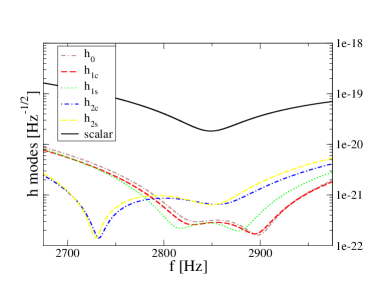
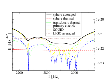
Figure 5: On the left, all the GW quadrupolar modes and the scalar one. On the right, the sky-averaged sensitivity of the sphere (along with the various noise contributions), compared to that of LIGO.

Once the $h_{N}(\omega)$’s are transformed back in the time domain, six time series are obtained, which describe the noise corresponding to the components of the $5$ spheroidal modes of the tensor $h_{ij}$ and of the scalar mode, see eq. (45). However, given the poor sensitivity of the detector to the latter (see fig. 5), this channel is bound to contain instrumental noise only and it will be dropped in the forthcoming analysis.

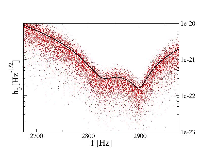
Figure 6: The mode $h_{0}$ as it has been reconstructed starting from an actual noise realization, superimposed with its expectation value.

III The analysis pipeline

We have now the five time series corresponding to the quadrupolar modes, which are enough and necessary to reconstruct the most general symmetric, traceless $3\times 3$ matrix.

Still this is a redundant description of a GW, and we will exploit this redundancy to discriminate between real GW signals and excitations of the modes due to disturbances other than gravitational.

The treatment in this section closely follows the exposition of Foffa:2008pm , which is summarized here.

III.1 The scalar trigger

If one knew exactly the form of the expected signal, the optimal strategy would be to perform a multidimensional matched filter as follows:

$$h_{N}(\omega)\rightarrow(h^{sig}\cdot h)_{S}\,,$$ (48)

where the $h^{sig}_{N}(\omega)$’s are the Fourier modes of the quadrupolar components of the expected signal, and we have introduced the following notation:

$$(X\cdot Y)_{S}\equiv X^{{\dagger}}_{N}(\omega)\cdot(S^{h})^{-1}_{NN^{\prime}}(\omega)\cdot Y_{N^{\prime}}(\omega)\quad N,N^{\prime}=0\,,\dots\,,4\,.$$ (49)

However in a realistic case neither the temporal dependence of the signal, nor the arrival direction are known. One could think of overcoming this difficulty by doing several matched filters with signal of various shapes and polarizations, and coming from several directions in the sky, but this method is computationally very intensive, and in addition results in a much higher false alarm rate than the method we are going to describe now.

We would like to find triggers out of the stretch of data, without need of a detailed knowledge of the signal. This has been done in Foffa:2008pm by building the following quantity:

$$H(\omega)\equiv(h\cdot h)_{S}\,.$$ (50)

The Fourier transform of this quantity is then fed to a suitably adapted version of WaveBurst, the event trigger generator used in the LIGO data analysis Klim ; Klim2 . The WaveBurst algorithm make use of the wavelet decomposition, and among the bank of wavelet packets we picked the Symlet base with filter length sixty Mal .

If a GW signal is present in the $h_{N}$’s, WaveBurst will detect it in $H$ whatever its shape, polarization and arrival direction, provided of course, that it is strong enough.

Once the trigger has been established the analysis is performed on the modes $h_{N}$’s, by collecting for each trigger the values of the wavelet coefficients. At this point the arrival direction can be reconstructed by a likelihood method analysis. This is different than what is being done by the Coherent WaveBurst algorithm Klimenko:2008fu , where the likelihood value is computed at every point of the time-frequency plane, as we do not have the sufficient computational power to perform such a daunting task. On the other hand, as it will be shown in sec. IV, adopting the above mentioned scalar trigger allows a good detection efficiency and reduce enormously the computational cost of the procedure, as our algorithm runs on a standard MacPro machine with two 3GHz processors and it takes for the analysis a time which is roughly two thirds of the actual time duration of the data.

The values of $\theta,\phi$ of the GW arrival direction are then found as the ones maximizing the likelihood function. This method identifies an arrival direction of the candidate GW event no matter if a real GW has excited the detector or a glitch, say, has taken place. To confirm this direction determination we combine it with a different, algebraic method. When the two methods do not determine the same directions, within some tolerance to be discussed quantitatively in sec. IV, the event can be discarded as spurious.

Figure 7: Example of event trigger. Sine-gaussian GW injection, centered at $t=500$sec, width $50$msec, central frequency $2825$Hz and strength $h_{rss}=7\times 10^{-21}{\rm Hz}^{-1/2}$. On the left is the $H$ mode defined in eq. (50), and on the right the likelihood of eq. (56) on the points of the trigger.

III.2 Likelihood method for direction reconstruction

The probability of having a given stretch of data $\{h_{N}\}$ assuming a GW with polarization amplitudes $h_{+}$ and $h_{\times}$ from the direction identified by the usual polar angles $\theta,\phi$, is often referred as likelihood function and is denoted by $p(\{h_{N}\}|H_{\zeta_{N}})$. For stationary, Gaussian, white noise with zero mean, and by taking into account that the noises in the different channels are correlated, such probability is

$$p(\{h_{N}\}|H_{\zeta_{N}})\propto\exp\left[-((h-\zeta)\cdot(h-\zeta))_{S}/2\right]\,,$$ (51)

where $\zeta_{N}$ is defined as

$$\zeta_{N}=F_{N}^{+}(\theta,\phi)h_{+}+F_{N}^{\times}(\theta,\phi)h_{\times}\,,$$ (52)

$F_{N}^{+,\times}$ being the pattern function of the $N$ mode for the $+,\times$ polarization.

Following the standard procedure Flanagan:1997kp ; Anderson:2000yy , the likelihood ratio $\Lambda$ can be defined as

$$\Lambda(h_{+,\times},\theta,\phi)=\frac{p(\{h_{N}\}|H_{\zeta_{N}})}{p(\{h_{N}\}|H_{0})}\,.$$ (53)

By maximizing the likelihood ratio eq. (53) with respect to $h_{+},h_{\times}$ a function $\mathcal{L}(\theta,\phi)$ of the angles alone is found

$$\begin{array}[]{l}\displaystyle\!\!\!\!\!\!\!\!\!\!\!\!\!\!\!\!\!\!\!\!\mathcal{L}_{h}(\theta,\phi)=\frac{1}{2}\left[(F^{+}\cdot F^{+})_{S}(F^{\times}\cdot F^{\times})_{S}-(F^{+}\cdot F^{\times})^{2}_{S}\right]^{-1}\times\\ \!\!\!\!\!\!\!\!\!\!\!\!\!\!\!\!\!\!\!\!\displaystyle\left[F^{\times}\cdot F^{\times})_{S}(h\cdot F^{+})^{2}_{S}+(F^{+}\cdot F^{+})_{S}(h\cdot F^{\times})^{2}_{S}-2(h\cdot F^{+})_{S}(h\cdot F^{\times})_{S}(F^{+}\cdot F^{\times})_{S}\right]\,.\end{array}$$ (56)

Maximizing the likelihood ratio is equivalent to maximizing the posteriori probability $p(H_{\zeta_{N}}|\{h_{N}\})$ in the case of flat priors. We then take the values of $\theta,\phi$ (which enter the expression for the $F_{N}$’s) maximizing $\sum_{\{trigger\}}\mathcal{L}_{h}(\theta,\phi)$, that is the sum of the likelihood over every point of time-frequency plane exceeding the threshold, as our estimation of the arrival direction of the candidate event.

III.3 Determinant method for direction reconstruction

Another method to reconstruct the direction of arrival GW by exploiting the (redundancy of the) five quadrupolar modes is based on linear algebra considerations Merkowitz:1997qc . A general metric perturbation in the transverce-traceless gauge is necessarily parametrized by a symmetric, traceless $3\times 3$ matrix with zero determinant. No matter which arrival direction nor polarization, the null eigenvector always points to the arrival direction (with the usual ambiguity in up and down direction).

As the quadrupolar modes allow full reconstruction of the metric perturbation, we have an independent method to identify the incoming direction of the signal.
Of course none of the eigenvalues is expected to be exactly zero at every point in the trigger, we then proceed to order the three eigenvalues $\lambda_{i}$ so that $|\lambda_{0}|\leq|\lambda_{1}|\leq|\lambda_{2}|$ and define the following quantity

$$r\equiv\frac{\sqrt{2}|\lambda_{0}|}{\sqrt{\lambda_{1}^{2}+\lambda_{2}^{2}}}\,.$$ (57)

For a perfect GW-like $r$ vanishes, thus the smallest it is, the less the noise is contaminating the GW signal. If for at least one point in the trigger $r<r_{0}$, with $r_{0}$ a suitably chosen threshold, a direction can be identified by associating to the signal the direction designated by the eigenvector relative to the smallest eigenvalue $\lambda_{0}$.

For each point of the trigger satisfying the condition $r<r_{0}$ a direction is identified; the average is then taken by weighting them with the factor $1/r$ in order to obtain a single direction for each trigger.

IV Test of the method

IV.1 Setup and calibration

In order to test the efficiency of our method, we injected mock GW signals in the five channels corresponding to the spheroidal components of $h_{ij}$ (see subsection II.3).

As efficiency is a good measure of the validity of the method only in presence of an estimate of the false alarm rate, we also injected non-GW signals which are supposed to mimic the presence of non-Gaussian noise in the data.

In both cases the amplitude shape is a sine Gaussian

$$h_{inj}(t+t_{0})=h_{0}e^{-t^{2}/(2\Delta^{2})}\sin(2\pi ft)$$ (58)

where $\Delta=0.05$sec, $f=2825$Hz, $t_{0}$ is the signal center and $h_{0}$ is determined by the signal $h_{rss}$.

Four sets of injections (of 50 signals each) have been done both for GW and non-GW signals, with amplitudes $h_{rss}=\{3,5,7,10\}\cdot 10^{-21}{\rm Hz^{-1/2}}$, corresponding to $SNR\simeq 16,27,37,53$ in amplitude, see figure 8.

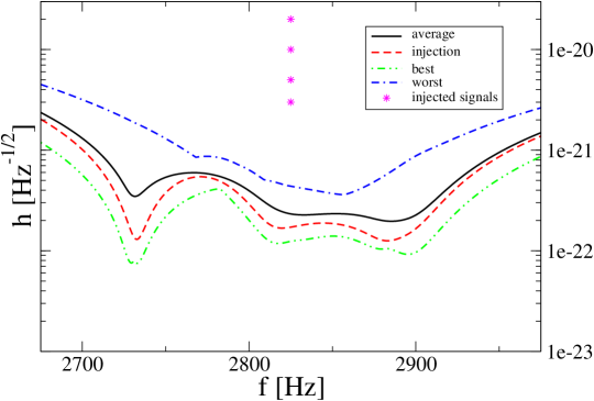
Figure 8: The stars indicate the injections, while the dashed line is the strain sensitivity for the arrival direction of the injections. For comparison, we have displayed also also the averaged sensitivity (continuous line), as well as the ones corresponding, at any given value of the frequency, to the best and worst possible directions.

For the mock GW signals, the amplitude distribution among the different channels corresponds to linearly polarized GW’s (either $+$ or $\times$) with arrival direction $\theta=54.736^{\circ},\phi=45^{\circ}$, while for non-GW signals the amplitude is distributed randomly on the different channels and normalized to ensure the required $h_{rss}$.

For each injection detected by the trigger, the arrival direction has been reconstructed by the two methods (likelihood and determinant) explained in sec. III and the event have been selected only when the two methods had a discrepancy below some threshold $\delta$.

A ROC curve can be constructed to assess what is the best value for $\delta$: for each set of injections one can define the efficiency as the fractional number of injections which are recovered and for which the two different direction identification methods give directions separated by less than $\delta$. By measuring the efficiency for GW and non-GW injections and plotting the former vs the latter for different values of $\delta$, fig. 10 has been obtained, where the four curves refers to the four different signal strengths.

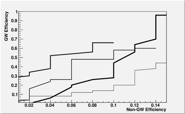
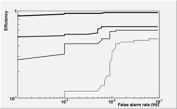
Figure 9: Detection efficiency of GW-injections vs. detection efficiency of non-GW signals obtained by varying the maximum allowed distance between the two different direction reconstruction methods. Lines of increasing thickness correspond to injections sets of increasing amplitude, $h_{rss}=\{3,5,7,10\}\times 10^{-21}{\rm Hz}^{-1/2}$.

Figure 10: Detection efficiency of GW-injections vs. false alarm rate of events on the data with just intrinsic detector noise, obtained by varying the maximum allowed distance between the two different direction reconstruction method. Lines of increasing thickness correspond to injections sets of increasing amplitude, $h_{rss}=\{3,5,7,10\}\times 10^{-21}{\rm Hz}^{-1/2}$.

The same can be done comparing the GW detection efficiency with the false alarm rate obtained analyzing the data containing only Gaussian noise (i.e. without any injection): the plot is reported in fig. 10 and shows that, contrarily to what happens in fig. 10, the ROC curve shows a strong dependence on $\delta$, especially at low $h_{rss}$ (notice that the scales of the two figures are different).

This calibration enabled us to set at $\delta_{thr}=0.2$ rad as the optimal value; all the results reported in the remaining part of the paper have been obtained with $\delta=\delta_{thr}$.

IV.2 Results

IV.2.1 Likelihood only

As a first step, we want to check what is the significance of finding a trigger on the scalar mode $H$ defined in eq. 50. In Fig. 11 we report the distribution of the likelihood values for the triggers obtained in correspondence of GW and non-GW injections. Mean values and sigmas for the likelihood are reported in tab. 1.

We see that our algorithm detects more efficiently GW injections rather than non-GW ones, but at this stage it is impossible to discriminate a priori between the two kinds of injections.

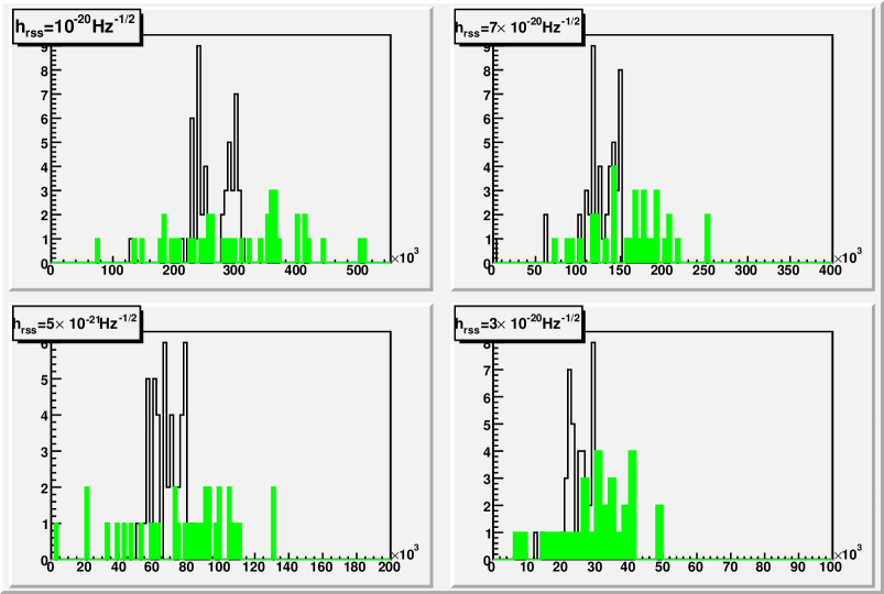
Figure 11: Distribution of the values of the likelihood function for GW-injections (empty-black) and for non-GW injections (filled-green) for various $h_{rss}$.

$h_{rss}{\rm(Hz^{-1/2})}$	GW			non-GW
	#inj/#trigg	$\mu$	$\sigma$	#inj/#trigg	$\mu$	$\sigma$
$10^{-20}$	50/50	$2.6\times 10^{5}$	$3.5\times 10^{4}$	41/50	$3.0\times 10^{5}$	$9.8\times 10^{4}$
$7\times 10^{-21}$	48/50	$1.3\times 10^{5}$	$2.7\times 10^{4}$	33/50	$1.6\times 10^{5}$	$4.3\times 10^{4}$
$5\times 10^{-21}$	45/50	$6.7\times 10^{4}$	$9.5\times 10^{3}$	34/50	$7.7\times 10^{4}$	$3.1\times 10^{4}$
$3\times 10^{-21}$	37/50	$2.5\times 10^{4}$	$4.1\times 10^{3}$	30/50	$3.1\times 10^{4}$	$1.0\times 10^{4}$

Table 1: Number of injections detected, mean and $\sigma$ for the distribution of the likelihood values for the GW and non-GW injections

IV.2.2 Likelihood + determinant

We now complete the maximum likelihood method with a cross check in order to get rid of spurious events: this is achieved by means of the geometrical method described in subsection III.3.

The major effect of this cross check is that in some cases the value of the parameter $r$ defined in eq.(57) is above the threshold that we had chosen, $r_{thr}=0.05$, which implies that a direction reconstruction through the linear algebra method is simply not meaningful. When this happens (in most of the non-GW injections and in a few GW ones), the trigger is discarded.

In Figs. 13,13 we report the distribution of distances between different direction reconstructions, see also tab. 3, while fig. 14 shows graphically the result of the direction reconstruction with the different methods for the GW injections. As expected (see Zhou:1995en , Stevenson:1996rw ), the precision in the determination of the arrival direction degrades at decreasing SNR.

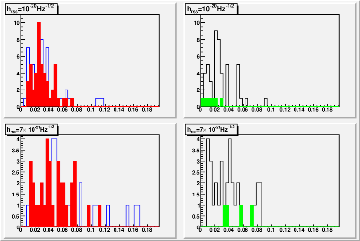
Figure 12: Distribution of the distances between the injection direction and the direction reconstructed by the likelihood method (left, filled-red), injection direction and the one reconstructed by the determinant method (left, empty-blue), and between likelihood and determinant reconstructed directions (right,empty-black), for $h_{rss}=10$ (up) and $7$ (down) $\cdot 10^{-21}{\rm Hz}^{-1/2}$. Also is displayed the distance in the direction determination for non GW-injections (right, filled-green).

Figure 13: Same as Fig. 13 for $h_{rss}=5$ (up) and $3$ (down) $\cdot 10^{-21}{\rm Hz}^{-1/2}$.

	GW
$h_{rss}(10^{-21}{\rm Hz^{-1/2}})$		i-l		i-d		l-d
	#det/#trigg	$\mu$	$\sigma$	$\mu$	$\sigma$	$\mu$	$\sigma$
10	48/50	0.031	0.015	0.037	0.026	0.027	0.018
7	33/48	0.048	0.024	0.062	0.040	0.040	0.023
5	30/45	0.068	0.035	0.089	0.055	0.063	0.036
3	24/37	0.11	0.053	0.19	0.21	0.15	0.18

Table 2: Number, mean and $\sigma$ for the distributions of distances between injection direction and likelihood reconstructed (i-l), injection and determinant reconstructed (i-d), likelihood and direction (l-d) for GW injections for different signal strengths.

	non-GW
$h_{rss}(10^{-21}{\rm Hz^{-1/2}})$	#det/#trigg	$\mu$	$\sigma$
10	8/41	0.014	0.0089
7	5/33	0.050	0.016
5	7/34	0.13	0.14
3	9/30	0.13	0.11

Table 3: Number, mean and $\sigma$ for the distributions of distances between likelihood and determinant reconstructed directions for non-GW injections for different signal strengths.

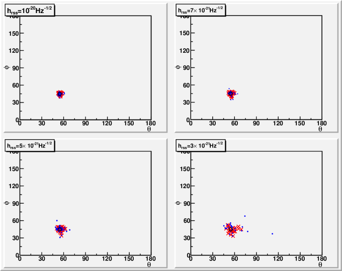
Figure 14: Each graph correspond to 50 linearly polarized injections of a signal (25$+$, 25$\times$). The black circle marks the injection direction, red crosses indicate direction reconstructed with the likelihood method, blue dots are obtained via the determinant method.

Finally, the application of the cut to eliminate triggers with $\delta>\delta_{thr}$ does not change much the situation at this stage: we found indeed that when a direction reconstruction is possible, this is almost always compatible with the one found with the likelihood algorithm.

Figure 15 shows the final detection efficiency for all the sets of injections: it should be noted that the efficiency for non-GW seems not to depend on the signal SNR, which points towards the fact that they ”survived” the cuts simply because they had by chance a GW-like geometrical configuration.

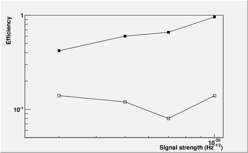
Figure 15: Detection efficiency of GW-injections (filled squares) and of non-GW signals (empty squares) as a function of the injected signal strength. The triggers surviving all the cuts are (in order of decreasing SNR) 48,33,30 and 21 for the GW injections, and 7,4,6 and 8 for non-GW.

V Conclusions

We have set up an algorithm which exploits the multichannel capability of the sphere in such a way to filter spurious disturbances. We have tested our method on various sets of injections of GW and non-GW signals over a Gaussian background noise which reproduces a possible outcome of the six transducers of a spherical detector like miniGRAIL.

We found that by crossing the two direction reconstruction methods, the false alarm rate due to Gaussian noise can be reduced to ${\cal O}(10^{-2}\div 10^{-3}{\rm Hz}^{-1})$ and that the detection efficiency for non-Gaussian noise (the non-GW injections) is $5-10$%, independently of the SNR. These results can be achieved while keeping the detection efficiency for GW signals in the range $50-95$%.

Moreover as summarized in tab. 3, the arrival direction of the gravitational wave can be determined with good accuracy on the trigger satisfying our cross-check, with a precision which ranges from roughly $0.2$ rad ($\simeq 10^{o}$) at SNR$\simeq 16$ to rapidly improve with the signal strength up to $0.03$ ($\simeq 2^{o}$) at SNR$\simeq 53$.

References

transducers’ azimuth	$\theta_{k=0,1,2}$	$37.3773^{\circ}$
transducers’ azimuth	$\theta_{k=3,4,5}$	$79.1876^{\circ}$
transducers’ longitude	$\varphi_{k=0,1,2}$	$(1+2k)*60^{\circ}$
transducers’ longitude	$\varphi_{k=3,4,5}$	$2k*60^{\circ}$
transducers’ frequencies	$\omega_{k=0,1}$	2863 Hz
transducers’ frequencies	$\omega_{k=2,3}$	2850 Hz
transducers’ frequencies	$\omega_{k=4,5}$	2878 Hz
transducers’ masses	$m_{k=0,1}$	0.205 Kg
transducers’ masses	$m_{k=2,3}$	0.153 Kg
transducers’ masses	$m_{k=4,5}$	0.150 Kg
transducers’ quality factors	$Q_{k=0\dots 6}$	$1\times 10^{6}$
gap electric fields	$E_{k=0\dots 5}$	$2\times 10^{7}V/m$
effective resistances	$r_{k=0,1}$	0.0883 Ohm
effective resistances	$r_{k=2,3}$	0.1140 Ohm
effective resistances	$r_{k=4,5}$	0.0872 Ohm
total capacities	$C_{k=0,1}$	1.1638$\times 10^{-9}$ F
total capacities	$C_{k=2,3}$	0.6978$\times 10^{-9}$ F
total capacities	$C_{k=0,1}$	1.1935$\times 10^{-9}$ F
primary inductances	$L^{p}_{k=0\dots 5}$	0.3595 H
secondary inductances	$L^{s}_{k=0\dots 5}$	2.1$\times 10^{-6}$ H
auto-inductances	$M^{ps}_{k=0\dots 5}$	1$\times 10^{-8}$ H
SQUID’s input inductances	$L^{i}_{k=0\dots 5}$	1.7$\times 10^{-6}$ H
SQUID’s self inductances	$L^{SQ}_{k=0\dots 5}$	8$\times 10^{-11}$ H
SQUID’s mutual inductances	$M^{SQ}_{k=0\dots 5}$	1$\times 10^{-10}$ H
SQUID’s shunt resistances	$R^{sh}_{k=0\dots 5}$	20 $\Omega$

Table 5: Readout specifications

References

- (1) H. J. Weber, Phys. Rev. 117 (1960) 306.
- (2) www.ligo.caltech.edu, www.virgo.infn.it, www.geo600.uni-hannover.de, tamago.mtk.nao.ac.jp .
- (3) www.auriga.lnl.infn.it, www.roma1.infn.it/rog .
- (4) J. A. de Freitas Pacheco, C. Filloux and T. Regimbau, Phys. Rev. D 74 (2006) 023001 [arXiv:astro-ph/0606427].
- (5) P. Astone et al., Class. Quant. Grav. 23 (2006) S169.
- (6) P. Astone et al. [IGEC-2 Collaboration], Phys. Rev. D 76 (2007) 102001 [arXiv:0705.0688 [gr-qc]].
- (7) L. Baggio et al. [AURIGA Collaboration], arXiv:0710.0497 [gr-qc].
- (8) V. Fafone, J. Phys. Conf. Ser. 39 (2006) 42.
- (9) M. Bonaldi, M. Cerdonio, L. Conti, A. Ortolan, G. A. Prodi, L. Taffarello and J. P. Zendri, Prepared for 28th International Cosmic Ray Conferences (ICRC 2003), Tsukuba, Japan, 31 Jul - 7 Aug 2003.
- (10) L. Gottardi et al., Phys. Rev. D 76 (2007) 102005 [arXiv:0705.0122 [gr-qc]].
- (11) O. D. Aguiar et al., Class. Quant. Grav. 23 (2006) S239.
- (12) R. V. Wagoner and H. J. Paik (1977). In Experimental Gravitation, Proceedings of the Pavia International Symposium, Accademia Nazionale dei Lincei, Roma.
- (13) C. Z. Zhou and P. F. Michelson, Phys. Rev. D 51 (1995) 2517.
- (14) E. Coccia, J. A. Lobo and J. A. Ortega, Phys. Rev. D 52, 3735 (1995).
- (15) J. A. Lobo and M. A. Serrano, Europhys. Lett. 35, 253 (1996).
- (16) T. R. Stevenson, Phys. Rev. D 56 (1997) 564.
- (17) S. Foffa and R. Sturani, Class. Quant. Grav. 25 (2008) 184036 [arXiv:0805.0718 [gr-qc]].
- (18) S. M. Merkowitz and W. W. Johnson, Phys. Rev. D 56 (1997) 7513 [arXiv:gr-qc/9706062].
- (19) S. M. Merkowitz, Phys. Rev. D 58 (1998) 062002 [arXiv:gr-qc/9712079].
- (20) J. A. Lobo, Mon. Not. Roy. Astron. Soc. 316 (2000) 173 [arXiv:gr-qc/0006109].
- (21) M. A. Gasparini and F. Dubath, Phys. Rev. D74 (2006), 122003.
- (22) L. Gottardi, Phys. Rev. D 75 (2007), 022002.
- (23) M. Maggiore, “Gravitational Waves. Vol. 1: Theory and Experiments”, Oxford University Press, October 2007. 572p.
- (24) C. D. Tesche and J. Clarke, J. Low.Temp. Phys. 29 (1977) 301; C. D. Tesche and J. Clarke, J. Low.Temp. Phys. 37 (1979) 397;
- (25) S. Klimenko, I. Yakushi, M. Rakhmanov and G. Mitselmakher, 2004 Class.Quant.Grav. 21 S1685.
- (26) S. Klimenko and G. Mitselmakher, 2004 Class.Quant.Grav. 21 S1819.
- (27) E. E. Flanagan and S. A. Hughes, Phys. Rev. D 57 (1998) 4566 [arXiv:gr-qc/9710129].
- (28) W. G. Anderson, P. R. Brady, J. D. E. Creighton and E. E. Flanagan, Phys. Rev. D 63 (2001) 042003 [arXiv:gr-qc/0008066].
- (29) S. Klimenko, S. Mohanty, M. Rakhmanov and G. Mitselmakher, Phys. Rev. D 72 (2005) 122002 [arXiv:gr-qc/0508068].
- (30) S. Klimenko, I. Yakushin, A. Mercer and G. Mitselmakher, arXiv:0802.3232 [gr-qc], to appear in the proceedings of GR18: 18th International Conference on General Relativity and Gravitation 7th Edoardo Amaldi Conference on Gravitational Waves Amaldi7), Sydney, Australia, 8-13 Jul 2007.
- (31) Mallat S. ”A wavelet tour in signal processing”, Academic Press, 1998, chap. VII.
Appendix A: detector parameters