Memory Effects and Transport Coefficients for Non-Newtonian Fluids

Abstract

We discuss the roles of viscosity in relativistic fluid dynamics from the point of view of memory effects. Depending on the type of quantity to which the memory effect is applied, different terms appear in higher order corrections. We show that when the memory effect applies on the extensive quantities, the hydrodynamic equations of motion become non-singular. We further discuss the question of memory effect in the derivation of transport coefficients from a microscopic theory. We generalize the application of the Green-Kubo-Nakano (GKN) to calculate transport coefficients in the framework of projection operator formalism, and derive the general formula when the fluid is non-Newtonian.

1 Non-Newtonian Nature of a Dissipative Fluid in Relativistic Regime

The effect of dissipation in relativistic fluids is one of current topics in the physics of relativistic heavy-ion collisions [1]. Here, we discuss this problem focusing on the memory effect on irreversible current. It is well-known that in a simple covariant extension of the Navier-Stokes theory there appears the problem of relativistic acausality and instability associated with it. First let us illustrate using the example of diffusion equation, the basic idea of memory effect as the solution for the problem of acausality in relativistic hydrodynamics.

In the usual derivation of diffusion equation, we assume that the irreversible current $J(t)$ is simply proportional to the corresponding thermodynamic force $F(t)$,

$$J(t)=DF(t),$$ (1)

where $D$ is a transport coefficient. The fluid whose irreversible current posseses this property is referred to as a Newtonian fluid, and the evolution is described by, for example, the Navier-Stokes equation. However, to be exact, there should exist some time retardation effect in generating the current in the medium, when a thermodynamic force is applied (remember the linear response theory). The expression (1) is justified only when there is clear separation of microscopic and macroscopic scales and the retardation effect is negligible. This assumption is usually satisfied in fluid around us, where the average velocity of molecules is larger than the velocity of the sound, but the speed of a fluid diffusion is much slower.

However, depending on the fluid, there exist many counter examples of this Newtonian behavior. There, the clear separation of microscopic and macroscopic timescales disappear due to the correlations, and we should consider the retardation effect in the definition of relativistic irreversible currents,

$$J(t)=\int_{-\infty}^{t}G(t-s)F(s),$$ (2)

where $G(t)$ is a memory function which represents the retardation effect.

Another situation where the Newtonian nature is not obvious is the motion of viscous fluids in relativistic regime. There, the fluid can be accelerated up to the speed of light and the proper time is slowed down due to the Lorentz retardation. Therefore, the effect of retardation, even small in non-relativistic regime, becomes crucial in the dynamics of a viscous fluid. Therefore, to include the retardation effects in the formulation of viscous hydrodynamics is a natural step to extend the fluid dynamics in the relativistic regime and, as a matter of fact, this extension is crucially related to the problem of acausality as seen below.

Let us consider a diffusion process [3]. Then the thermodynamic force is given by the spatial derivative of a conserved density $n$ and the linear relation (1) is called Fick’s law. By substituting Fick’s law into the equation of continuity, we obtain the diffusion equation. As is well known, the diffusion equation has a problem of infinite propagation speed. On the other hand, when we use Eq. (2) with a simple exponential memory function,

$$G(t)=\frac{D}{\tau_{R}}e^{-t/\tau_{R}},$$ (3)

where $\tau_{R}$ is the relaxation time and $D$ is the diffusion constant, we obtain a telegraph equation and then the maximum propagation speed is given by $\sqrt{D/\tau_{R}}$. It is also worth for mentioning that what we can obtain from microscopic dynamics is not the diffusion equation but the telegraphic equation [3].

The same discussion is applicable to relativistic dissipative hydrodynamics [2]. In the relativistic Navier-Stokes (Landau-Lifshitz) equation, the viscous flows are defined by assuming Eq. (1). For example, in the bulk viscosity, the corresponding thermodynamic force is $\partial_{\mu}u^{\mu}$, where $u^{\mu}$ is the fluid velocity. Thus the bulk viscosity is given by

$$\Pi=-\eta\partial_{\mu}u^{\mu}.$$ (4)

On the other hand, in the hydrodynamics consistent with causality, it is given by

$$\pi(\tau)=\int_{-\infty}^{\tau}G(\tau-s)\partial_{\mu}u^{\mu}(s),$$ (5)

where $\tau$ is a proper time. As is shown in Ref. [4, 5], the propagation speed of signal exceeds the speed of light in the case of Eq. (4), and this acausality makes the hydrodynamic evolution unstable. On the other hand, hydrodynamic motion with a covariant formulation of the retarded irreversible current (5) becomes causal and stable. Due to the acausality and associated instability problem, it is impossible to apply the Landau-Lifshitz theory in a physical system without using artificial tricks (such as to use the value of $\partial_{\mu}u^{\mu}$ of the former step in the time-integration algorithm).

2 Memory Effects on Extensive Measures

Another important mechanism is the finiteness of fluid cells to be applied thermodynamic relations [6]. In the derivation of hydrodynamics, it is assumed that the local equilibrium is achieved in each fluid cells which has finite spatial extension (to be rigorous, it should be infinite compared with the microscopic scale). Then, the second law of thermodynamics and the memory effect should be applied on extensive measures associated with this finite volume. To introduce an extensive measure for the density of an additive quantity, let us consider a fluid cell of proper volume $V.$ Due to the fluid flow, this volume changes in time and its time rate of change is given by

$$\frac{1}{V}\frac{dV}{dt}=\nabla\cdot\vec{v},$$

where $\vec{v}$ is the fluid velocity field. This equation can be written in a covariant form as

$$\partial_{\mu}(\sigma(\mathbf{r},t)u^{\mu}(\mathbf{r},t))=0,$$ (6)

where $\sigma(\mathbf{r},t)$ is the inverse of the volume of the fluid cell at $\mathbf{r}$, and $u^{\mu}$ is the fluid velocity. Then the irreversible current is given by

$$\frac{J(t)}{\sigma(t)}=\int_{t_{0}}^{t}dsG(t-s)\frac{F(s)}{\sigma(s)}$$ (7)

This is equivalent to the solution of the following differential equation,

$$\tau_{R}\frac{d}{dt}J(t)+J(t)=DF(t)-\tau_{R}J(t)\partial_{\mu}u^{\mu}(t).$$ (8)

Noted that this result does not depend on the choice of the volume of the fluid cell $\sigma(t)$. The above equation differs from that of the so-called Maxwell-Cattaneo equation (or in fluid mechanics, the truncated Israel-Stewart theory),

$$\tau_{R}\frac{d}{dt}J(t)+J(t)=DF(t)$$ (9)

which can also be obtained from the memory effect applied on the current density itself as

$$J(t)=\int_{t_{0}}^{t}dsG(t-s)F(s).$$

The last non-linear term in (8) is important not only for the physical concept of the irreversible current, but also for the stability of relativistic fluids. Actually there are two different origins for instabilities in relativistic dissipative hydrodynamics. One is the instability induced by acausality which we addressed in the previous section (Here we would like to call attention that, it is sometimes considered that the problems of acausality and instability are different problems but as shown in Ref. [5], the instability of relativistic fluids is induced by acausality itself), which can be removed even by the truncated Israel-Stewart theory (9). The other instability appears in ultra-relativistic phenomena even the theory is causal. When the term $\partial_{\mu}u^{\mu}$ becomes very large, the bulk viscosity $\Pi$ can take a very large negative value. In such extreme situation, we can analytically show that the mass matrix associated with the simple causal dissipative hydrodynamics Eq.(9) becomes negative, hence it is unstable [6].

On the other hand, such a instability never appears when we consider the non-linear term in Eq.(8). This is because, the presence of the non-linear term prevents the bulk viscosity to become negatively very large. We found that there exist the minimum value of $\Pi$, given by [6]

$$\Pi\geq-\frac{\zeta}{\tau_{R}},$$ (10)

where $\zeta$ is the bulk viscosity coefficient and $\tau_{R}$ is the corresponding relaxation time. Due to this condition, the mass matrix of the hydrodynamic equation is proved to be positive definite. Thus the causal dissipative hydrodynamics with finite size effect is stable even for ultra-relativistic phenomena.

Another important fact is that, the so-called full Israel-Stewart theory can also be expressed in terms of a memory function. However, in this case a very peculiar form of thermodynamic quantity should be taken to apply the memory effect and the physical interpretation from the extended thermodynamic point of view is difficult [6].

In Fig. 1, we show the shock formation with an initial velocity $\gamma=5$. As is shown in the left panel, in this ultra-relativistic initial condition, the causal dissipative hydrodynamics without the finite size effect becomes unstable. On the other hand, if the finite size effect is taken into account, the instability disappears.

A very different scenario where relativistic fluid dynamics can be applied is found in astrophysics. The speed of flow becomes $\gamma\sim 100$ in the Gamma-raybursts. Thus, the construction of the dissipative hydrodynamics applicable to such an extreme situation is important for some astrophysical processes, too.

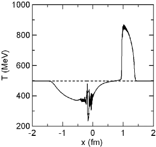
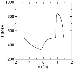
Figure 1: The temperature in the shock formation calculated without the finite size effect (left) and with the finite size effect (right), starting from the homogeneous initial condition (dotted line) [6].

3 GKN formula : Applicable to non-Newtonian Fluids ?

As we have shown, it is natural to consider that the behavior of a fluid in relativistic regime is non-Newtonian type. This means that we cannot use various techniques which are developed to analyze the Newtonian fluids. The Green-Kubo-Nakano (GKN) formula to derive the transport coefficients is one of them. The GKN formula has been applied to calculate the viscosity coefficients and the heat conductivity of the quark-gluon plasma. However, it should be noted that the assumption of Newtonian fluids is implicitly used in the derivation of the expressions. Thus those values of transport coefficient obtained from the usual GKN formula might not be applicable to be used in the relativistic regime. We have to consider how the non-Newtonian nature affects the values of transport coefficients.

To see this, we consider the system whose Hamiltonian is given by $H$. By applying an external force, the total Hamiltonian is changed from $H$ to $H+H_{ex}(t)$, with

$$H_{ex}(t)=-AF(t),$$ (11)

where $A$ is an operator and $F(t)$ is the c-number external force.

We consider the current $J$ induced by the external force. In the framework of the linear response theory, we can write

$$\langle J\rangle=\int_{-\infty}^{t}ds\Psi(t-s)F(s),$$ (12)

where the response function is given by

$$\Psi(t)=\int_{0}^{\beta}d\lambda\langle\dot{A}(-i\lambda)J(t)\rangle_{eq},$$ (13)

where $\beta=1/T$ and $T$ is the temperature. This is the exact result in the sense of the linear approximation and one of the important expressions of the GKN formula. However, when we define transport coefficients of hydrodynamics for the non Newtonian fluid, we need to take care to use this expression.

In applying the GKN formula for hydrodynamic transport coefficients, we assume the relation between currents and the external force such as $J(t)=D_{GKN}F(t)$ which define the transport coefficient $D_{GKN}$. One can immediately see that this is nothing but the assumption of Newtonian fluids. Commonly the formula to calculate this $D_{GKN}$ in this way is usually called the “GKN formula” of the shear viscosity, the bulk viscosity, heat conduction and so on. To derive the expression for $D_{GKN}$, we have to ignore the memory effect (time-convolution integral) in Eq. (12),

$$\langle J\rangle\approx\int_{0}^{\infty}ds\Psi(s)F(t).$$ (14)

Then the GKN formula is reduced to

$$D_{GKN}=\int_{0}^{\infty}ds\Psi(s).$$ (15)

In the case of shear viscosity, this is given by the time correlation function of energy-momentum tensor.

In principle, we can derive the formula for non-Newtonian transport coefficients by assuming Eq.(8) instead of Eq.(1). From the exact result Eq.(12), we can derive the following equation,

$$\partial_{t}J(t)=\Psi(0)F(t)+\int_{0}^{\infty}ds\partial_{s}\Psi(s)F(t).$$ (16)

In the second term, we ignore the time-convolution integral. In the first order approximation in the relaxation time, we may use the usual GKN formula to re-express the first term. Then we finally obtain

$$\partial_{t}J(t)=\frac{\Psi(0)}{D_{GKN}}J(t)+\int_{0}^{\infty}ds\partial_{s}\Psi(s)F(t).$$ (17)

By comparing this equation with Eq. (8) ignoring the non-linear term, we can derive the expression of $D$ and $\tau_{R}.$ The results obtained in this way differ from those of the direct application of GKN formulas to Newtonian fluid. However, in the limit of Markovian approximation of the correlation function, the two results coincide.

Strictly speaking, the shear viscosity is induced not by the external force but by the difference of the boundary conditions. Actually, the GKN formula of the shear viscosity is derived by using the nonequilibrium statistical operator method proposed by Zubarev. Thus the discussion we developed here is not directly applicable to the problems discussed in this paper. More detailed discussion and the exact expression of the non-Newtonian transport coefficients are given in [7, 8].

We have investigated the viscous fluid dynamics emphasizing the memory effect. When a fluid posses a non-Newtonian behavior, the use of GKN formula should be cautious.

We thank fruitful discussion with G.Denicol and Ph. Mota on the extensivity of the memory effects. This work has been supported by PRONEX, FAPERJ and CNPq.

References

- [1] See for example, M. Luzum, P. Romatschke, Phys.Rev.C78, 034915, 2008; R. Baier, P. Romatschke, D. T. Son, A. O. Starinets and A. Stephanov, JHEP 0804, 100, 2008; P. Romatschke and U. Romatschke, Phys.Rev.Lett. 99, 172301, 2007; U. W. Heinz and Huichao Song, J.Phys.G35, 104126, 2008; T. Hirano, U.W. Heinz, D. Kharzeev, R. Lacey and Y. Nara, J.Phys. G35, 104124, 2008.
- [2] T. Koide, G. S. Denicol, Ph. Mota, and T. Kodama, Phys. Rev. C75, 034909 (2007) .
- [3] T. Koide, Phys. Rev. E72, 026135 (2005).
- [4] G. S. Denicol, T. Koide, T. Kodama and Ph. Mota, Phys. Rev. C78, 034901 (2008).
- [5] G. S. Denicol, T. Koide, T. Kodama and Ph. Mota, J. Phys. G35 115102 (2008).
- [6] G. S. Denicol, T. Koide, T. Kodama and Ph. Mota, arXiv:0808.3170.
- [7] T. Koide, Phys. Rev. E75, 060103(R) (2007).
- [8] T. Koide and T. Kodama, Phys. Rev. E 78, 051107 (2008).