Compensation driven superconductor-insulator transition

Abstract

The superconductor-insulator transition in the presence of strong compensation of dopants was recently realized in La doped YBCO. The compensation of acceptors by donors makes it possible to change independently the concentration of holes $n$ and the total concentration of charged impurities $N$. We propose a theory of the superconductor-insulator phase diagram in the ($N$, $n$) plane. It exhibits interesting new features in the case of strong coupling superconductivity, where Cooper pairs are compact, non-overlapping bosons. For compact Cooper pairs the transition occurs at a significantly higher density than in the case of spatially overlapping pairs. We establish the superconductor-insulator phase diagram by studying how the potential of randomly positioned charged impurities is screened by holes or by strongly bound Cooper pairs, both in isotropic and layered superconductors. In the resulting self-consistent potential the carriers are either delocalized or localized, which corresponds to the superconducting or insulating phase, respectively.

I Introduction

The superconductor-insulator (SI) transition remains a challenging and controversial subject after more than two decades Fisher ; Finkelshtein ; Hebard ; Goldman ; MaLee ; Nandini ; Mason ; Gantmakher ; Shahar ; Meir ; Baturina ; Kapitulnik ; FeigelmanIoffeKravtsov . In the low temperature limit one can drive the SI transition by changing the film thickness, the magnetic field, or the concentration of electrons in gated devices. In high $T_{c}$ superconductors such as YBCO one can tune the concentration of holes by changing the oxygen doping. This leads to a SI transition at small hole concentrations of about 6$\%$ per Cu site in the CuO plane. From this perspective, YBCO is essentially a heavily doped semiconductor. It is well known that upon decreasing the doping a semiconductor undergoes the metal-insulator transition when the three-dimensional concentration of dopants $N$ crosses the threshold $Na^{3}\approx 0.02$. Here $a=\hbar^{2}\kappa/me^{2}$ is the effective Bohr radius, $\kappa$ is the dielectric constant, $m$ is the effective mass and $e$ is the proton charge. In under-doped high $T_{c}$ superconductors the conducting phase is a superconductor, and one expects a superconductor-insulator transition at a similar threshold concentration of dopants.

In semiconductors one can vary the concentration of carriers and impurities independently using compensation. For example, in a $p$-type semiconductor doped with $N_{A}$ monovalent donors compensation means addition of a concentration $N_{D}<N_{A}$ of donors, so that the concentration of remaining holes $n=N_{A}-N_{D}$ becomes much smaller than the total concentration of charged impurities $N=N_{A}+N_{D}$. The metal-insulator transition in the ($N$, $n$)-plane of a compensated semiconductor was studied long ago. It was shown SE ; SEbook that in heavily doped samples with $Na^{3}\gg 1$ the transition takes place when $n(N)\sim N/(Na^{3})^{1/3}$, as was later verified by experiments (cf., Fig. 13.3 in Ref. SEbook, ).

Recently Ando it was demonstrated that YBCO crystals can also be strongly compensated by doping with La. Although many of the La³⁺ ions substitute for Y³⁺ and are therefore not electrically active, some La³⁺ ions substitute for Ba²⁺ and hence play the role of monovalent donors compensating oxygen acceptors. It was shown that the sample of $\rm{Y_{1-z}La_{z}(Ba_{1-x}La_{x})_{2}Cu_{3}O_{y}}$ with $x=0.13$ and z = 0.62 is completely compensated at $y=6.32$, and becomes $n$-type at $y<6.32$. Thus, also in high $T_{c}$ superconductors the concentration of impurities and holes can be varied independently. Resistance measurements Ando showed that the SI transition point non-trivially depends on both $x$ and $y$. In strongly compensated samples it occurs at much larger concentration of holes than in standard uncompensated samples. However, the full phase diagram of the zero-temperature SI transition in the plane ($N$, $n$) has not been established yet experimentally. In this paper we predict it theoretically.

I.1 Global phase diagram

Let us start by discussing the gross features of the phase diagram which are expected, e.g., in compensated high $T_{c}$ materials such as La doped YBCO, see Fig. 1. In the uncompensated material with $n=N$, we expect a transition from the insulator to a superconductor at a critical doping $n_{u}$ (on the underdoped side) as discussed above. The pairing mechanism is believed to be at least in part due to spin fluctuations which become significantly weaker upon exceeding an optimal doping level. Finally, superconductivity is essentially destroyed on the overdoped side $(n>n_{o})$, or at least $T_{c}$ is strongly suppressed. Upon adding the temperature axis to the phase diagram this leads to the well-known superconducting dome in high temperature superconductors. As disorder is increased by compensation (increasing $N/n$), the doping concentration $n_{u}(N)$ where delocalized states first appear, increases as well. On the other hand, we expect that the upper critical density $n_{o}(N)$ decreases because usually disorder diminishes the effectiveness of the superconductive attraction, while it enhances the competing Coulomb repulsion. We thus propose that at some compensation $N/n=N^{*}/n$ where $n_{u}(N^{*})=n_{o}(N^{*})=n^{*}$ there may exist a tricritical point beyond which a direct transition from a localized insulator to a metal without intermediate superconducting state takes place. Note that the effect of compensation is similar to that of a strong magnetic field: both suppress superconductivity.

In this paper we are not concerned with the transition to a metal at high doping, nor with the vicinity of the tentative tricritical point $T=\{n_{u}(N^{*}),N^{*}\}$ in Fig. 1, where metal, insulator and superconductor meet. Instead we analyze the dependence of $n_{u}$ on the degree of compensation. In the case of strong coupling superconductivity the latter exhibits interesting new features in the regime of low densities, reflecting the crossover from a BEC (Bose-Einstein condensate) to a BCS superconductor in the interacting gas of preformed Cooper pairs.

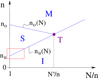
Figure 1: Global phase diagram of compensated high $T_{c}$ superconductors in the plane $(n,N)$. Here M, S and I stand for metal, superconductor and insulator, respectively. The line $n_{u}(N)$ separates the insulator form a superconductor, which eventually turns into a metal upon overdoping beyond $n_{o}(N)$. We conjecture the existence of a tricritical point $T=\{n_{u}(N^{*}),N^{*}\}$, where $n_{u}(N^{*})=n_{o}(N^{*})$ beyond which the insulator turns directly into a metal. A large part of the paper is focused on the lower left corner of the line $n_{u}(N)$ which exhibits features of the BEC-to-BCS crossover of the interacting gas of Cooper pairs in strong coupling superconductors.

I.2 BEC-to-BCS crossover in the SI transition

A first attempt to predict the low density part of the SI phase diagram Boris was based on the toy model of an isotropic compensated $p$-type semiconductor with a strong (unspecified) pair-forming mechanism. The size of hole pairs $\xi$ was taken as a free parameter as determined by a strong coupling mechanism. For the major part of this paper we will adopt this approach as well. For simplicity we assume $\xi$ to be independent of the density of carriers and the disorder, at least in the dilute BEC part of the phase diagram. However, it would not be difficult to account for such a dependence (in certain strong coupling models for preformed pairs one expects such a dependence even in the dilute regime FeigelmanIoffeKravtsov ). In the following we thus concentrate on the two independent variables $n$ and $N$, taking $\xi$ as a fixed parameter.

In Ref. Boris, two limiting cases of the SI transition were identified: In the limit of large pairs which overlap significantly in space, $n\xi^{3}\gg 1$, one obtains the standard Bardeen-Cooper-Schrieffer (BCS) instability of the fermion system. If disorder is weak the electrons are delocalized and form a dirty BCS superconductor. This happens essentially at the same critical density as the metal-insulator transition in a semiconductor SE ; SEbook without superconductivity,

$$n=n_{1}(N)=\frac{N}{(Na^{3})^{1/3}}.$$ (1)

Note that there is no dependence on $\xi$ in (1), because electrons are only weakly bound and, therefore, screen the random potential of charged impurities like free ones. Here and in all formulae below we omit numerical coefficients and adopt the scaling approach. The scaling is controlled by the large dimensionless parameter $Na^{3}\gg 1$ and the dimensionless ratio $a/\xi$.

The opposite limit of very small and strongly bound pairs is more unusual. Upon decreasing the concentration of holes $n$ the SI transition occurs due to the localization of hole pairs (composite bosons) in a random potential Fisher . At small external disorder the bosons undergo a Bose-Einstein condensation (BEC) while at large disorder the condensate is fragmented and turns into a Bose insulator (also referred to as Bose glass). This limit is reached when the pairs are dilute, $n\xi^{3}\ll 1$, and can be considered as a gas of point-like charged bosons. A similar picture applies to the case of neutral bosons BorisCold ; Nattermann .

As we will rederive below, for point like bosons the border between the superconducting BEC phase and the Bose insulator occurs at the hole density

$$n=n_{3}(N)=\frac{N}{(Na^{3})^{1/5}},$$ (2)

where typical screened Coulomb wells loose their bound quantum levels. Of course, the length $\xi$ is again irrelevant, because the pairs are considered as point-like bosons. Notice that for a heavily doped system with $Na^{3}\gg 1$, we have $n_{3}(N)\gg n_{1}(N)$. In other words, in a given disorder, a system of small pairs delocalizes at a much higher density $n$ than a system of weakly bound electrons with larger pair size $\xi$. This reflects the fact that, at equal density $n$, bosons have less kinetic energy, and thus one needs more of them to induce their collective delocalization.

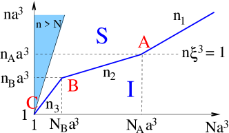
Figure 2: SI-phase diagram in an isotropic 3D system, on a log-log plot (S stands for superconductor, I for insulator). The dilute boson part of the curve (C-B) is described by $n_{3}$, Eq. (2), the interacting boson part (B-A) by $n_{2}$, Eq. (19), and the standard strong coupling BCS transition beyond A by $n_{1}$, Eq. (1). The BEC part of the transition line (C-A) only exists if the pairs are very small, $\xi<a$. In the case of larger pairs ($\xi>a$), and for weak coupling in general, the $n_{1}$ line extends all the way to the point C. The shaded region corresponds to $n>N$ which is unphysical.

The crossover between the above two limiting cases is quite subtle. In Ref. Boris, it was incorrectly assumed that the limits described by $n_{1}(N)$ and $n_{3}(N)$ require only the inequalities $n\xi^{3}\gg 1$ or $n\xi^{3}\ll 1$ to be valid, and hold all the way up to the BEC-BCS crossover line $n\xi^{3}=1$. However, this argument neglected the repulsion between bosons as they become denser, and thus it lead to the incorrect conclusion that the BEC-BCS crossover line forms a substantial part of the SI transition line. Below we reconsider this crossover in detail.

This paper contains two main new results. First, in Sec. II we show that while $n_{1}(N)$ is valid all the way up to the BEC-BCS crossover line $n\xi^{3}=1$, the BEC part of the SI transition is to a large extent dominated by an intermediate segment $n=n_{2}(N)$ of the transition line at which the chemical potential of repulsive compact bosons becomes of the order of the amplitude of the screened Coulomb potential. This segment interpolates between the above discussed limits $n_{1}(N)$ and $n_{3}(N)$, see Fig. 2. We will see that the BEC regime, $n_{2}(N)$ and $n_{3}(N)$, occurs only when the pairs are smaller than the effective Bohr radius, $\xi<a$. We show below that in this case transport in the insulating phase is due to the hopping of hole pairs. In App. A we will discuss bipolarons as an example of strong coupling superconductivity which can give rise to such small pairs.

Second, in Sec. III we apply similar ideas to a generic strongly anisotropic superconductors with a layered structure, such as formed by the CuO or FeAs planes in high $T_{c}$ superconductors. We arrive at a qualitatively similar phase diagram in the plane ($N$, $n$) for this case as well, see Fig. 4. The details of the phase diagram are found to depend on the ratio between Bohr radius and interlayer distance.

II SI phase diagram of an isotropic superconductor

Let us now recall the derivation of the limiting critical concentrations $n_{1}(N)$ and $n_{3}(N)$. We consider the case of heavily doped materials, $Na^{3}\gg 1$, which provides a large parameter that makes the scaling analysis well controlled.

II.1 BCS segment of the superconductor-insulator transition line

We start from the BCS side at high density (large pairs). Let us divide the sample into cubes of linear size $R$. Due to spatial fluctuations of the concentrations of donors and acceptors each cube contains a random impurity charge of arbitrary sign and with an absolute value of the order of $e(NR^{3})^{1/2}$. At the scale $R$ such randomly fluctuating charges create a random potential energy relief of amplitude

$$eV(R)\sim\frac{e^{2}(NR^{3})^{1/2}}{\kappa R}=\frac{e^{2}(NR)^{1/2}}{\kappa}.$$ (3)

This energy diverges at large $R$, so that screening even by a small concentration of holes $n$ is crucial. To discuss this screening we estimate the characteristic fluctuating density $\delta N(R)$ of impurity charges at the scale scale $R$:

$$\delta N(R)=\frac{(NR^{3})^{1/2}}{R^{3}}=\left(\frac{N}{R^{3}}\right)^{1/2}.$$ (4)

The concentration $n$ of carriers can be redistributed between wells and hills of the random potential. This redistribution screens all the scales $R$ for which $\delta N(R)\leq n$ or, in other words, for $R\geq R_{s}$, where

$$R_{s}=\left(\frac{N}{n^{2}}\right)^{1/3}$$ (5)

is the nonlinear screening radius SE ; SEbook . All scales $R<R_{s}$ remain unscreened, because even when all electrons are transferred from all the hills of the potential energy to all its wells they are not able to level off the charge density of such fluctuations. Since $V(R)\propto R^{1/2}$ among remaining scales the most important contribution to the random potential is given by $R=R_{s}$. Thus, the amplitude of the nonlinearly screened random potential energy is

$$eV(R_{s})=\frac{e^{2}}{\kappa}\frac{N^{2/3}}{n^{1/3}}.$$ (6)

So far we have dealt only with the electrostatic energy of holes and neglected their kinetic energy. At $T=0$ all kinetic energy is of quantum origin, and we should find the conditions under which it is small enough so that the above described picture of localized electrons is valid. Clearly the potential energy Eq. (6) is able to localize electrons with concentration $n$ if it is larger than the Fermi energy of holes in its wells $\epsilon_{F}(n)=\hbar^{2}n^{2/3}/2m$ ($m$ being the effective mass). In the opposite case $\epsilon_{F}(n)\gg eV(R_{s})$ the Fermi sea covers the typical maxima of the potential energy relief and the semiconductor behaves like a good conductor, see Fig. 3. Equating $eV(R_{s})$ and $\epsilon_{F}(n)$ we obtain the critical concentration $n_{1}(N)$ for the SI transition, as given by Eq. (1) SE ; SEbook . Note that the non-linear screening theory requires $nR_{s}^{3}=N/n\gg 1$ which is always fulfilled in strongly compensated materials.

In the delocalized phase electron screening becomes linear, the screening radius being given by the standard Thomas-Fermi expression

$$r_{s}=\left(\frac{1}{e^{2}}\frac{d\mu}{dn}\right)^{1/2}=\frac{a}{(na^{3})^{1/6}},$$ (7)

and the amplitude of the screened potential relief equals $eV(r_{s})=e^{2}(Nr_{s})^{1/2}/\kappa$. As expected, at the transition $n=n_{1}$, these two quantities match the corresponding expressions Eq. (5) and Eq. (6) pertaining to the insulating side.

II.2 BEC segments of the superconductor-insulator transition line

In the above discussion the notion of strong pairing attraction and preformed pairs was irrelevant. However, as we follow the transition line Eq. (1) to lower densities, we may finally reach the crossover to the BEC regime, which takes place when strongly bound hole pairs become dilute, i.e., when $n_{1}\xi^{3}=(Na^{3})^{2/3}(\xi/a)^{3}=1$. This corresponds to the point $A$ in Fig. 2 and the densities

$$n_{A}^{(3d)}a^{3} = (a/\xi)^{3},$$ (8)

$$N_{A}^{(3d)}a^{3} = (a/\xi)^{9/2}.$$ (9)

Under the assumption of heavy doping, $Na^{3}\gg 1$, the crossover to the BEC regime can only happen when the pair size is much smaller than the Bohr radius, $\xi<a(Na^{3})^{-2/9}<a$. For the sequel we will assume that the pairs are very small $\xi<a$. Since we will be using the concept of strongly bound pairs a lot, we briefly recall the essential elements of strong coupling superconductivity.

II.2.1 Strong coupling superconductivity

The physics of a fermion gas subject to attractive interactions (but in the absence of disorder) has been studied in detail in Refs. Eagles, ; Leggett, ; NS, , and is now a very active field of studies in the context of cold atoms PhysRep . The authors of Ref. NS, considered electrons with a mutually attractive potential of size $V_{k,k^{\prime}}\sim V$ for $k\leq k_{0}$, and rapidly decaying for larger $k$. If the interaction potential between two holes is too weak to produce a bound state ($V<V_{c}\sim 1/mk_{0}$), the fermions are essentially unbound, and only an exponentially narrow range of energies around the Fermi level participates in pairing, the gap being of the order of

$$\Delta\approx\frac{4k_{F}^{2}}{m}\exp[-1/\nu(E_{F})V_{k_{F},k_{F}}],$$ (10)

where $\nu(E_{F})$ is the density of states at the Fermi level. On the other hand, if the mutual interaction is strong, bound states of two single carriers exist, and at low density the fermions organize into preformed pairs with a typical size $\xi\approx[(V/V_{c}-1)k_{0}]^{-1}$ and a pairing energy $E_{\rm pair}\sim\hbar^{2}/m\xi^{2}$. As long as the pairs are dilute, $n\xi^{3}\ll 1$, the chemical potential for the addition of pairs, $\mu$, and the gap function $\Delta$ are much smaller than the pairing energy,

$$\mu \sim E_{\rm pair}\,(n\xi^{3})\sim\frac{\hbar^{2}}{m}n\xi,$$ (11)

$$\Delta \sim E_{\rm pair}\,(n\xi^{3})^{1/2}.$$ (12)

However, when the pairs become dense, the pair chemical potential is dominated by the Fermi energy of its constituting fermions,

$$\mu\simeq E_{F}=\frac{\hbar^{2}n^{2/3}}{m}.$$ (13)

At the same time the gap function $\Delta$ crosses over to its strong coupling BCS form, i.e., Eq. (10) with an exponent of order footnote1 $O(1)$,

$$\Delta\sim E_{F}.$$ (14)

In this dense regime the pairing energy is dominated by the gap function $E_{\rm pair}\approx\Delta>\hbar^{2}/m\xi^{2}$.

II.2.2 Very dilute bosons

In order to derive the critical concentration $n_{3}(N)$ of Cooper pairs (charge $2e$ bosons) at the SI transition, we notice that the above calculation of the nonlinear screening radius $R_{s}$ (5) and the random potential energy created by screened charged impurities (6) remains unaltered in the scaling sense.

The difference between the gas of composite bosons and that of weakly bound fermions lies in their quantum kinetic energy Boris . Due to the weak effect of Pauli’s principle on strongly bound Cooper pairs, a large number of them can occupy a given localized level of a potential well, keeping the quantum kinetic energy low. Therefore, the condition of delocalization of Cooper pairs is much more stringent than the condition $eV(R_{s})<\epsilon_{F}(n)$ which applies to fermions. A sufficient condition for the delocalization of a compact Cooper pair is that a typical well of the random potential does not contain any localized level, or $eV(R_{s})<\hbar^{2}/mR_{s}^{2}$, where $m$ is the effective mass of pairs, which we assume to be of the same order as that of electrons. This condition is also necessary if mutual repulsions can be neglected, as we will discuss below. Solving the equation

$$eV(R_{s})=\frac{\hbar^{2}}{mR_{s}^{2}},$$ (15)

for $n$ and using Eqs. (5) and (6) we find the critical concentration of the SI transition given in Eq. (2). This derivation clearly demonstrates why $n_{3}(N)\gg n_{1}(N)$. According to Eq. (6) the potential energy amplitude $eV(R_{s})$ decreases with increasing $n$. To achieve delocalization it has to be pushed below the quantum kinetic energy of the clean system. This requires larger $n$ in the boson case and thus leads to $n_{3}(N)\gg n_{1}(N)$.

II.2.3 Moderately dilute, interacting bosons

So far, following Ref. Boris, , we have taken into account all the Coulomb interactions. However, we have neglected the short range repulsive interaction between composite bosons. Such a repulsion is related to the Fermi nature of individual holes, which becomes important if two pairs of holes overlap within their length $\xi$. This short range interaction can be described by the well-known expression for the chemical potential $\mu(n)$ of a non-ideal gas of bosons of concentration $n$ with a scattering length $\xi$:

$$\mu=(\hbar^{2}/m)n\xi,$$ (16)

which is also confirmed by the result (11) for dilute systems of strong coupling superconductivity. This chemical potential reflects the extra quantum kinetic energy due to the mutual repulsion of the pairs. Note that it matches the Fermi energy $E_{F}=\hbar^{2}n^{2/3}/m$ when the BEC-BCS crossover $n\xi^{3}=1$ is reached.

The delocalization criterion (15) discussed above remains relevant as long as the density is low enough such that $\mu$ is smaller than the typical localization energy $\hbar^{2}/mR_{s}^{2}$. However, at an impurity density $N=N_{B}$, the chemical potential of the critical insulator ($n=n_{3}(N)$) becomes of the order of the typical amplitude of the random Coulomb potential Eq. (6). This marks the point $B$ in Fig. 2, beyond which the delocalization is driven by the mutual repulsion between bosons. The crossover in the transition line occurs at the densities

$$n_{B}^{(3d)}a^{3} = (a/\xi)^{2},$$ (17)

$$N_{B}^{(3d)}a^{3} = (a/\xi)^{5/2}.$$ (18)

On the low density side the $n_{3}(N)$ line ends at point $C$ which corresponds to the uncompensated limit $n_{3}a^{3}=Na^{3}=1$. At higher densities, $N>N_{B}$ we need to compare the quantum kinetic energy Eq. (16) to the amplitude of potential fluctuations, Eq. (6), similarly as in the BCS regime. This leads to the new segment of the transition line

$$n=n_{2}(N)=\frac{N^{1/2}}{(a\xi)^{3/4}},$$ (19)

which interpolates between points $A$ and $B$ in Fig. 2.

We can confirm this result by calculating the linear screening radius $r_{s}$ in the delocalized Bose gas. Using Eq. (16) to compute the compressibility we find the Thomas-Fermi screening radius from Eq. (7) as $r_{s}=(a\xi)^{1/2}$. One easily verifies that this linear screening radius matches the non-linear screening radius (5) at the transition line (19). Similarly, one can check that along the line $n_{1}$ the linear screening radius of the conducting side matches the non-linear screening radius $R_{s}$ on the insulating side. The linear screening in the very dilute superfluid above the line $n_{3}$ is found Boris to be

$$r_{s}=\left(\frac{a}{n}\right)^{1/4},$$ (20)

which again matches $R_{s}$ at the transition line $n_{3}$.

The fact that the SI transition line undergoes a kink at the BCS-BEC crossover is very similar to the case of the superfluid-insulator phase transition in a neutral gas of attractive fermions BorisCold . However, at lower density $n_{2}$ lies below the BCS-BEC crossover line, contrary to what was claimed in Ref. Boris, .

The results obtained so far in this section can be summarized in the following concise manner: The chemical potential of a gas of composite bosons of size $\xi$ , localized into a region of linear size $R$ is given by

$$\mu(n,R)=\max\left[\frac{\hbar^{2}}{mR^{2}},\frac{\hbar^{2}}{m}n\min(\xi,n^{-1/3})\right].$$ (21)

The first term of the righthand side refers to the ground state energy in a well of size $R$. At higher density $\mu(n,R)$ is dominated by the second one, describing the interaction energy (16) of repulsive bosons (for $n\xi^{3}<1$), and the Fermi energy $E_{F}\sim n^{2/3}$ of the BCS regime (for $n\xi^{3}>1$), respectively.

The SI transition occurs when the chemical potential dominates over the amplitude of the screened impurity potential, i.e., when

$$\mu(n,R_{s})\sim eV(R_{s}).$$ (22)

This can be reformulated as

$$\max\left[\left(\frac{n}{n_{3}(N)}\right)^{\frac{5}{3}},\,\frac{n}{n_{1}(N)}\min[1,(n\xi^{3})^{\frac{1}{3}}]\right]=1,$$ (23)

which defines the transition line in the whole $(n,N)$-plane, as plotted in Fig. 2.

II.3 The nature of the insulating regime

II.3.1 Droplets in the insulator

It is important to understand the insulating phase in some more detail. Deep in the insulator, the charge density $n$ is by no means homogeneously distributed. Instead the holes or Cooper pairs fill deep wells, where they form puddles of high density, while the rest of the space is completely void of carriers.

To determine the chemical potential and the size of puddles we can argue as follows: when $n\ll n(N)$ only the deep wells of the landscape are populated with carriers (see Fig. 3).

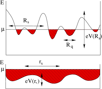
Figure 3: Top: Droplets in the insulator. The carriers assemble in non-percolating fragments of size $R_{q}<R_{s}$. Bottom: In the conductor, the wells are not deep enough to localize the carriers. The latter delocalize due to their quantum kinetic energy, $\mu>V(r_{s})$ ($\mu=E_{F}$ in the BCS limit of dense pairs).

Suppose the carriers fill a well of linear size $R<R_{s}$. Its typical depth $eV(R)$ is given by Eq. (3) , and it contains an excess impurity charge of order $eQ(R)=e(NR^{3})^{1/2}$. Upon filling the well with carriers, their chemical potential raises continuously with respect to the bottom of the well. Assume that when the chemical potential reaches $eV(R)$ we have filled in $Q_{q}(R)$ particles. If $R$ is small, $Q_{q}(R)<Q(R)$, that is, the exclusion principle or the repulsion between bosons limits the number of carriers we can fill into the well. In large wells, we can at most fill in $Q(R)$ particles before turning the well into a hump. However, those larger wells will not be filled homogeneously with particles. Rather, they split into smaller droplets for which $Q_{q}(R)\approx Q(R)$. The latter relation defines SEbook a typical droplet size $R_{q}$:

$$\mu\left(n=n_{q}\equiv\frac{Q(R_{q})}{R_{q}^{3}}\right)=eV(R_{q}).$$ (24)

Here we have to use the expressions for the chemical potential given above in Eq. (21).

Analyzing the three regimes of the phase diagram (BCS side, repulsive bosons and very dilute bosons) we find the following results. When $n\xi^{3}>1$ ($N>N_{A}^{(3d)}$ on the transition line), $\mu$ is given by $E_{F}(n)$, and we find the droplet size SEbook

$$R_{q,1}=\frac{a}{(a^{3}N)^{1/9}}.$$ (25)

In the repulsive boson regime, $(N\xi^{3})^{2}<n\xi^{3}<1$ (or $N_{B}^{(3d)}<N<N_{A}^{(3d)}$ on the transition line), we find instead

$$R_{q,2}=(a\xi)^{1/2}.$$ (26)

Eventually, in the lowest density regime, $n\xi^{3}<(N\xi^{3})^{2}$ where the bosons do not significantly interact, $R_{q}$ is simply the typical localization radius in the disorder potential. It is obtained from $\hbar^{2}/mR^{2}\sim eV(R)$ as

$$R_{q,3}=\frac{a}{(a^{3}N)^{1/5}}.$$ (27)

In all three cases, the insulator consists mostly of puddles of size $R_{q}$ which are well separated and do not percolate. One can verify that the SI transition occurs when the droplets grow to the size of the non-linear screening radius, $R_{q}=R_{s}=(N/n^{2})^{1/3}$. Indeed, at this point droplets of size $R_{s}$ start to percolate, which induces the delocalization transition.

Note the remarkable fact that in all insulating regimes the density of carriers in the above droplets is the same as the critical density of the corresponding segment of the SI transition, $n_{q}=Q(R_{q})/R_{q}^{3}=n(N)$.

II.3.2 Level spacing in droplets

Before we turn to the role which droplets play in the transport properties of the insulator phase, we have to discuss the level spacing in a typical droplet. The typical cost to add another carrier into a droplet is $\delta=R_{q}^{-3}\,d\mu/dn(n=n_{q})$. This is essentially the level spacing of the considered droplet. Interestingly this quantity turns out to be equal to the charging energy $e^{2}/R_{q}$. This holds both in the dense BCS-like part and in the interacting boson regime of the phase diagram. In the very dilute boson regime, the quantity of interest is not the level spacing $\delta$, but the typical kinetic energy scale of a localized wavefunction, which again turns out to be equal to the charging energy $e^{2}/R_{q}$. Thus, for the above (spontaneously originating droplets) we do not have to distinguish between one-electron level spacing and charging energy.

This unique energy scale is important in determining whether all carriers are paired or whether it is energetically favorable to break up a pair and redistribute the constituting holes onto two different droplets. The cost of such a break up is the pairing energy, while the maximal energy gain is of order $\delta\sim e^{2}/R_{q}$. Thus the criterion for having all carriers paired up in the ground state is

$$\delta\sim e^{2}/R_{q}<E_{\rm pair}.$$ (28)

In the BEC regime the pairing energy is given by $E_{\rm pair}\sim\hbar^{2}/m\xi^{2}$. In the BCS regime it is even bigger, if the BCS coupling remains strong, see Eq. (14). Thus, if $\xi<a$, it is never favorable to break Cooper pairs, i.e. the insulating state is always a Bose glass. Moreover the droplets are actually superconducting at low enough temperatures. In tunneling experiments they should show a hard gap with coherence peaks on its shoulders, despite the absence of global phase coherence among the droplets.

II.4 Variable range hopping transport in the insulator

The above implies that for systems with small pairs, $\xi<a$, the low temperature transport is Efros-Shklovskii variable range hopping of Cooper pairs between droplets. This yields a conductivity

$$\sigma(T)=\sigma_{0}\exp\left[-\left(\frac{T_{\rm ES}}{T}\right)^{1/2}\right]\,,$$ (29)

with a characteristic temperature

$$T_{\rm ES}=2.8\frac{(2e)^{2}}{\kappa\ell_{2}},$$ (30)

where $\ell_{2}$ is the effective localization length of a Cooper pair. This prediction agrees qualitatively with experimental data Ando ; Andoprivate .

However, there is an exception to the above assertion that pairs prevail in the insulator if $\xi<a$. Namely, if the dimensionless BCS coupling $\lambda$ decreases with increasing density in the BCS regime, the pairing energy $E_{\rm pair}$ can become exponentially suppressed at high densities. (This presumably happens on the overdoped side of high $T_{c}$ superconductors.)

When $E_{\rm pair}\approx\Delta$ falls below the level spacing in typical droplets, $\delta$, it becomes favorable to break up pairs and redistribute the carriers on different droplets. One can verify that at the same time the parity gap (the extra cost for having an odd number of particles per droplet) becomes smaller than the level spacing MatveevLarkin . In this situation the ground state of the system is a Coulomb glass of unpaired fermions. Consequently, the low temperature transport is again of the form (29), but with a characteristic temperature

$$T_{\rm ES}=2.8\frac{e^{2}}{\kappa\ell_{1}},$$ (31)

which is roughly 8 times smaller than (30), because the localization length of a hole is about twice as big as that of a pair, $\ell_{1}\sim 2\ell_{2}$. When pairs are not very strongly bound ($\xi>a$), as well as in the case of weak coupling, only the BCS segment of the superconductor-insulator border survives. In the weak coupling case, it can easily happen that $E_{\rm pair}<\delta$ in the droplets of the insulator. In this case they contain odd or even numbers of holes, and the low temperature variable range hopping is dominated by unpaired holes.

So far we have not specified any particular strong coupling mechanism which leads to the preformed pairs on the insulating side of the SI transition. In App. A we discuss an explicit example of strong coupling superconductivity, which allows one to formulate a direct microscopic criterion for the condition $\xi<a$. As discussed above, the latter is necessary to observe the BEC part of the SI transition in a heavily doped system.

II.5 Coulomb correlation energy

As we saw above the long range Coulomb interactions considered within mean field approximation play a major role in our theory. However, the correlation energy produced by the Coulomb interaction between nearest neighbors has been neglected so far. We should thus make sure that corrections to the chemical potential due to Coulomb correlations are subdominant with respect to the leading term given in Eq. (21). According to Foldy Foldy the energy per particle in a disorder-free, Coulomb interacting Bose system in 3d is

$$u_{\rm Cb}=\frac{e^{2}}{a}{\rho_{s}^{-3/4}}=\frac{\hbar^{2}}{m}n^{2/3}\rho_{s}^{5/8}=\frac{\hbar^{2}}{m}n^{1/4}a^{-5/4},$$ (32)

where $\rho_{s}=(a^{3}n)^{-1/3}$. One can verify that this quantity is indeed smaller than $\mu(n,R_{s})$, along the whole SI phase transition line, consisting of the segments $n_{1}(N)$, $n_{2}(N)$ and $n_{3}(N)$.

III SI phase diagram of a layered superconductor

III.1 General theory

III.1.1 Non-linear screening in a layered system

In this section, we extend our previous arguments to the case of anisotropic layered superconductors. We assume that with respect to the motion along the $c$-axis ($z$-axis) all holes reside in the lowest spatial quantization mode of the narrow quantum wells defining the conducting $ab$-planes ($x,y$-plane) perpendicular to the $c$-axis. These parallel wells are located at a distance $d$ from each other, each well containing holes with the two-dimensional concentration $nd$. Impurities of both signs are randomly distributed between these narrow quantum wells. We assume again that a strong attraction between the holes of a given well leads to preformed pairs (composite bosons) with a size $\xi$ in the plane of the well. To simplify things we will first assume an isotropic dielectric constant $\kappa$. Modifications due to anisotropy will be discussed in the next subsection.

Let us define again the effective Bohr radius in the $ab$-plane, $a=\hbar^{2}\kappa/me^{2}$. For the insulating phase we need to understand the non-linear screening in a system containing impurities in the bulk and screening carriers confined to planes. There are two limits of this screening problem. When the non-linear screening radius is bigger than the distance between layers, $R_{s}>d$, we can use our results for the isotropic 3d case, cf. Eqs. (5,6). On the other hand if $d>R_{s}$, the potential fluctuations within each plane are screened independently. For these two cases we have obtained the phase diagrams of Fig. 4. The specific expressions for the various lines are derived below.

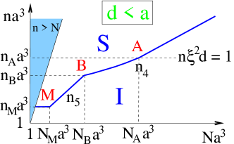
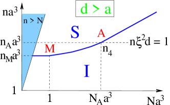
Figure 4: The superconductor-insulator transition in the plane $(n,N)$ for the model of a layered high $T_{c}$ superconductor (on a log-log scale). S stands for superconductor, I for insulator. The shaded region $n>N$ is unphysical. (a) Narrowly spaced layers, $d<a$. At lowest densities the SI transition is a Mott transition in the layers. The very dilute boson part of the curve (M-B) is described by $n_{5}$, Eq. (37), while the interacting boson and BCS parts (B-A and beyond) are described by $n_{4}$, Eq. (36). (b) Widely spaced layers, $d>a$. The dilute boson regime does not exist. In both cases, the point $A$ where a weak BEC-BCS crossover takes place, exists only if $(ad)^{1/2}>\xi$ or $a>\xi$, respectively.

The non-linear screening radius for the case $d>R_{s}$ has been derived in Refs. Gergel78, ; SE86, . Let us cover a conducting plane by densely packed cubes of linear size $R<d$. Fluctuations of the charge among these cubes are of the order of $e(NR^{3})^{1/2}$. The random potential they create in the planes can be screened by redistributing the charge of two-dimensional holes, $endR^{2}$ between potential hills and wells of linear size $R$, if the latter is large enough. We find the nonlinear screening radius $R_{s}$ by equating $e(NR^{3})^{1/2}=endR^{2}$, which yields

$$R_{s}=\frac{N}{(nd)^{2}}.$$ (33)

Only scales of the random potential with $R<R_{s}$ survive the screening. Thus, the amplitude of the remaining random potential is

$$eV_{s}=\frac{e^{2}}{\kappa}\frac{N}{nd}.$$ (34)

At small enough hole concentration $n$ the screening radius is always bigger than $d$. However, upon approaching the SI transition, either of the above screening scenarios may apply. As we will see, the first case applies to small separations of layers, $d<a$, while the screening of independent layers governs close to the SI transition if $d>a$.

III.1.2 Narrowly spaced layers, $d<a$

The difference between layered materials and isotropic ones is due to the confinement of the carriers to the layers. The quantum kinetic energy, or the chemical potential of pairs confined to a region of linear size $X$ in the plane, evaluates to

$$\mu(n,X)=\max\left[\frac{\hbar^{2}}{mX^{2}},\frac{\hbar^{2}}{m}\frac{nd}{\max\left[1,\log(1/\xi^{2}nd)\right]}\right].$$ (35)

Note that in 2d there is only a logarithmic difference between the Fermi energy $E_{F}$ in the fermion fluid and the interaction energy per particle in the Bose gas, both scaling essentially as $(\hbar^{2}/m)nd$. The logarithmic dependence of $\mu$ on the pair size $\xi$ in the interacting boson regime is well-known Schick71 . Note that the logarithm is replaced by unity at the BEC-BCS crossover point $nd\xi^{2}=1$. The first term in (35) is the kinetic energy of a single boson or fermion in a well of size $X$, the relevant size in the context of non-linear screening being $X=R_{s}$.

We will show below that the logarithmic effects due to the finite size of pairs $\xi$ is only relevant for the transition when the pairs are small, $\xi<(ad)^{1/2}$. Let us thus first discuss the opposite case $\xi>(ad)^{1/2}$. The chemical potential for pairs, Eq. (35), then scales in the same way as that for fermions without any superconducting correlations. Thus the results below describe equally well the metal-insulator transition of unpaired fermions confined to planes.

Delocalization and hence the insulator-conductor transition, takes place roughly when $\mu(n,R_{s})=eV_{s}$. In the high density regime where the Fermi energy dominates, the transition occurs at

$$n_{4}=\frac{N^{1/2}}{(ad)^{3/4}}.$$ (36)

The difference between this result and Eq. (1) is due to the confinement of holes to the $ab$-planes. At low densities, the random potential $eV_{s}$ competes against the kinetic energy due to the confinement of carriers to regions of size $R_{s}$ in the plane. ¿From this we find the critical density

$$n_{5}=\frac{N}{(Na^{3})^{1/5}},$$ (37)

which is the same as in the isotropic case, Eq. (2).

The line (2) continues down to densities $n_{M}=1/a^{2}d$ which is the minimal density required to drive a Mott transition in the layers. Note that for $d<a$ this minimal density is higher than in the isotropic case, since here the carriers are confined to narrowly spaced planes.

The crossover between $n_{4}(N)$ and $n_{5}(N)$ occurs at the densities

$$n_{B}^{(2d)}a^{3} = \left(\frac{a}{d}\right)^{2},\quad\quad N_{B}^{(2d)}a^{3}=\left(\frac{a}{d}\right)^{5/2}.$$ (38)

The transition lines $n_{4}$ and $n_{5}$ can also be derived by approaching from the conducting side, in close analogy to the isotropic case.

It is justified to deal with fermions and thus to ignore the logarithm in Eq. (35) if we are still on the BCS side of the BCS-BEC crossover, i.e., if $\xi^{2}nd>1$ down to $n=n_{B}^{(2d)}$. This condition is equivalent to $\xi>(ad)^{1/2}$ as we anticipated above. In this case, the crossover to the dilute boson (BEC) regime occurs along the line $n_{5}$ only, without affecting the shape of the SI transition line.

Let us now discuss effects which arise if fermions bind into small pairs of size $\xi<(ad)^{1/2}$. As in the isotropic case, there is a BCS-BEC crossover at the point $A$ in the phase diagram, where $n_{A}^{(2d)}=1/\xi^{2}d>n_{B}^{(2d)}$ and

$$n_{A}^{(2d)}a^{3} = \frac{a^{3}}{\xi^{2}d},\quad\quad N_{A}^{(2d)}a^{3}=\left(\frac{a}{d}\right)^{1/2}\left(\frac{a}{\xi}\right)^{4}.$$ (39)

However, here the difference between the fermion regime and the interacting boson regime results only in a logarithmic factor correcting the line $n_{4}$ to

$$n_{4}=\frac{N^{1/2}}{(ad)^{3/4}}\log^{3/4}\left(\frac{(ad)^{3/4}}{\xi^{2}dN^{1/2}}\right).$$ (40)

III.1.3 Widely spaced layers, $d>a$

If the spacing between layers is larger than the Bohr radius we need to compare the potential fluctuations (34) to the chemical potential (35). As above, we will find that when pairs are large, $\xi>a$, they do not affect the phase transition line, which then becomes equivalent to the metal-insulator transition of an unpaired fermion system. In the high density regime, equating $E_{F}$ to $eV_{s}$ from Eq. (34), we find the transition line

$$n_{4}=\frac{N^{1/2}}{a^{1/2}d}.$$ (41)

The non-linear screening radius remains constant $R_{s}=a$ along the SI transition line.

It turns out that, contrary to the case $d<a$ discussed above, the line (41) describes the SI transition down to dopant densities where $N_{M}a^{3}=1$ and $n=n_{M}=1/a^{2}d$, while the first term in (35) never becomes relevant. Once the dopants are dilute, $Na^{3}<1$, one leaves the regime of heavy doping. The potential for individual carriers is then dominated by the closest impurity charge. Under these conditions the delocalization takes place as a standard Mott transition in the planes. It occurs when the nearest neighbor distance in the planes is of order $a$, i.e., when

$$n=n_{M}=\frac{1}{a^{2}d}.$$ (42)

Again, it is justified to deal with fermions and to neglect logarithmic factors if $\xi^{2}nd>1$ holds down to $n=n_{M}$. This is equivalent to the condition of large pairs, $\xi>a$.

However, in the case where fermions are strongly bound into pairs of size $\xi<a$, there are logarithmic corrections to the phase boundaries. One finds that the line (41) turns slightly upward,

$$n_{4}=\frac{N^{1/2}}{a^{1/2}d}\log^{1/2}\left(\frac{a^{1/2}d}{\xi^{2}dN^{1/2}}\right),$$ (43)

for $n_{M}<n<n_{A}^{(2d)}=1/\xi^{2}d$. The full phase diagram is shown in Fig. 4b.

III.2 Anisotropic dielectric constant

Here we refine the above analysis and take into account the anisotropy of the dielectric constant in a layered system. We use $\kappa_{z}$ for $\kappa_{zz}$ and $\kappa_{x}$ for $\kappa_{xx}=\kappa_{yy}$. We also define the average dielectric constant as $\kappa=(\kappa_{x}^{2}\kappa_{z})^{1/3}$.

In order to derive the SI transition line in the presence of an anisotropic dielectric constant we first switch to the new coordinate frame $(x^{\prime},y^{\prime},z^{\prime})$, where $x^{\prime}=x/\kappa_{x}^{1/2}$, $y^{\prime}=y/\kappa_{x}^{1/2}$ and $z^{\prime}=x/\kappa_{z}^{1/2}$. In this frame LL the Coulomb interaction of a charged impurity with a hole becomes isotropic $e^{2}/\kappa^{3/2}r^{\prime}$. At the same time, the concentrations $N$ and $n$ are transformed, too: $N^{\prime}=\kappa^{3/2}N$, $n^{\prime}=\kappa^{3/2}n$.

Let us first treat the case of narrowly layered systems. In the new frame we have similarly to Eqs. (5,6) $R^{\prime}_{s}=N^{\prime 1/3}/n^{\prime 2/3}=N^{1/3}/\kappa^{1/2}n^{2/3}$ and $eV(R^{\prime}_{s})=e^{2}N^{\prime 2/3}/\kappa^{3/2}n^{\prime 1/3}=e^{2}N^{2/3}/\kappa n^{1/3}$. Thus, returning to the laboratory system we arrive back at Eq. (6) for the amplitude of the screened potential $eV_{s}$, and to the same SI transition line (36) with redefined $\kappa=(\kappa_{x}^{2}\kappa_{z})^{1/3}$. However, note that the notion of the nonlinear screening radius $R_{s}$ becomes anisotropic. Characteristic potential wells have a scale $X_{s}=\kappa_{x}^{1/2}R_{s}^{\prime}=(N^{1/3}/n^{2/3})\alpha^{1/6}$ in the $(x,y)$ plane, where $\alpha=\kappa_{x}/\kappa_{z}$. On the other hand, the scale perpendicular to the planes is $Z_{s}=\kappa_{z}^{1/2}R_{s}^{\prime}=(N^{1/3}/n^{2/3})\alpha^{-1/3}=X_{s}\alpha^{-1/2}<X_{s}$. This anisotropy modifies the critical concentration $n_{5}$ (i.e., the very dilute boson limit) to

$$n_{5}=\frac{\alpha^{1/5}N}{(Na^{3})^{1/5}}.$$ (44)

It also affects the criterion on the smallness of pairs that is required for a BEC regime with logarithmic factors to exist. The criterion follows from $n_{B}^{(2d)}\xi^{2}d<1$ where $n_{B}^{(2d)}$ is the crossing point of $n_{4}$ and $n_{5}$. This yields the requirement

$$\xi<\alpha^{1/6}(ad)^{1/2},\quad\quad(d<d^{*}).$$ (45)

The crossover from widely to narrowly spaced layers can be obtained from the criterion $Z_{s}=d$. It occurs at the spacing

$$d=d^{*}=\frac{\kappa_{z}}{\kappa}a=\alpha^{-2/3}a.$$ (46)

In the widely spaced case one finds

$$eV_{s}=\frac{e^{2}}{\kappa^{3/2}}\frac{N^{\prime}}{n^{\prime}d^{\prime}}=\frac{e^{2}}{\kappa^{3/2}}\kappa_{z}^{1/2}\frac{N}{nd},$$ (47)

and thus the corrected transition line

$$n_{4}=\left(\frac{\kappa_{z}}{\kappa}\right)^{1/4}\frac{N^{1/2}}{a^{1/2}d}=\alpha^{-1/6}\frac{N^{1/2}}{a^{1/2}d}.$$ (48)

The Mott transition at low density now takes place at a density

$$n_{M}=n_{B}^{(2d)}=\frac{1}{a_{x}^{2}d}=\frac{\alpha^{1/3}}{a^{2}d},$$ (49)

where $a_{x}=\alpha^{-1/6}a$ is the effective Bohr radius in the plane. It is obtained by comparing kinetic and Coulomb energy in the plane, $\hbar^{2}/ma_{x}^{2}=e^{2}/[\kappa^{3/2}a_{x}^{\prime}]=e^{2}/[\kappa^{3/2}(a_{x}/\kappa_{x}^{1/2})]$. Logarithmic corrections occur in this case if $n_{M}d\xi^{2}<1$, i.e., for

$$\xi<a\alpha^{-1/6},\quad\quad(d>d^{*}).$$ (50)

Note that the critical lines $n_{4}$ for narrowly and widely spaced systems match when $d=d^{*}$. The same holds for the critical size of pairs necessary to have a BEC-like regime.

III.3 Is the BEC limit of this theory applicable to high $T_{c}$ superconductors?

Above we have obtained results along two lines. First, for relatively large pairs (in the BCS regime) we predict the SI transition line given by Eqs. (36) and (37). Second, for small pairs we have discussed an additional logarithmic factor originating from BEC effects. One may question whether the value of $\xi$ in high $T_{c}$ superconductors is small enough so that the condition $nd\xi^{2}\leq 1$ for a BEC-like regime with extra logarithmic factors is realistic. The most frequently cited number for under-doped uncompensated YBCO for the superconducting coherence length is $2$ nm. However, for the case of strong coupling of holes the size of pairs, $\xi$, can be smaller than the coherence length. ARPES data in YBCO indicate that actually Campuzanoprivate $\xi\sim 1$nm. Using that that the boundary of the superconducting dome on the underdoped side occurs at $(n_{u}d)=0.06a^{-2}_{0}$ where $a_{0}\sim 0.4$nm is the lattice constant of the two-dimensional Cu lattice, one finds that the SI transition at $T=0$ empirically happens when $nd\xi^{2}\approx 0.4<1$. This means that the BEC part of our diagram Fig. 4 is marginally relevant. In iron-arsenide superconductors the small value $\xi<2$ nm was recently found Ong . Since $n_{u}da_{0}^{2}$ has a similar value as in cuprates, this leads to $n_{u}d\xi^{2}\sim 1$ in this new family of superconductors as well.

The low density (BEC) regime might indeed be experimentally relevant if one adopts a popular interpretation of the pseudogap which is observed in underdoped samples Randeria ; Uemura ; Deutscher ; Renner ; PhysRep ; Campuzano . The latter assumes that the pseudogap is due to preformed hole pairs with large binding energy ($E_{\rm pair}>T_{c}$), the pairs being localized by disorder at low doping density. If such an interpretation is correct, the small $N$ part of our diagram Fig. 4 may be relevant for high $T_{c}$ superconductors.

As we have seen the SI boundary reflects the BEC-BCS crossover in the form of extra logarithmic factors in the critical density $n_{4}$ only if $\xi$ is sufficiently small, i.e., if condition (45) or (50) is satisfied. Let us discuss this condition for the example of Bi₂Sr₂Cu₂O_6+δ (Bi-2201). The mean distance between copper planes is $d=12.3\AA$, and the lattice spacing in the planes is $a_{0}=5.36\AA$. From recent optical measurements vanHeumen , one can extract the effective mass of carriers as $m_{\rm eff}\approx 3-4m_{e}$ in the underdoped regime. The dielectric constant along the c-axis is BSCCO $\kappa_{z}=18.9$. We are not aware of direct measurements of $\kappa_{x}$, but usually, the anisotropy is relatively modest Tajima , e.g., $\alpha=\kappa_{x}/\kappa_{z}=0.99$ in Nd₂CuO₄, or $0.7$ in Pr₂CuO₄. Neglecting the anisotropy we can use $\kappa=\kappa_{z}$ and the effective mass to estimate the Bohr radius in Bi-2201 as $a\approx a_{x}\approx a_{z}\approx 3\AA$. We can compare this to an alternative estimate obtained as follows: We assume that the SI transition of uncompensated materials is essentially a Mott transition of doped carriers, which is known to occur roughly when MottDavis $(n_{u}d)a^{2}=c$ with fn2 $c\approx 0.04$. Using an approximate value for $n_{u}d\approx 0.06a_{0}^{-2}$ we find $a\approx 4.4\AA$, in rough agreement with the above calculation based on the effective mass. This material thus certainly corresponds to widely spaced layers, $d>a$. The estimated Bohr radius $a$ is of the same order as the typical pair size $\xi$ in strongly underdoped samples. The requirement (50) for observing the SI transition in the BEC regime is thus just marginally satisfied in this standard cuprate compound.

More favorable conditions for the crossover to the BEC limit may be expected in materials with high dielectric constants (such as in La_2-xSr_xCuO₄), which increases the Bohr radius. A similar tendency can be expected from a small effective mass (small band mass and/or small mass renormalization), provided it does not occur simultaneously with an increase of the pair size $\xi$.

The application of our theory to certain particular superconductors may require further adjustments of the model. For example, in $\rm{Y_{1-z}La_{z}(Ba_{1-x}La_{x})_{2}Cu_{3}O_{y}}$ acceptors are divalent and we have to define proper variables for the phase diagram. We can use $N_{A}=(y-6)/v_{\rm uc}$ for the concentration of divalent oxygen acceptors (excessive oxygen), $N_{D}=x/v_{\rm uc}$ for the concentration of monovalent donors, and $n=2N_{A}-N_{D}$ for the concentration of holes. Here $v_{\rm uc}$ is the volume of the unit cell. It is easy to show that the concentration $N=4N_{A}+N_{D}$ plays the role of the effective concentration of monovalent charged impurities. Indeed, for randomly distributed impurities in a given volume $R^{3}$, the variances of the donor, acceptor and net charge number distribution are equal to $N_{A}R^{3}$, $N_{D}R^{3}$ and $(p^{2}N_{A}+N_{D})R^{3}$ respectively, where $p$ represents the valence of the acceptor. So the effective concentration of monovalent charged impurities is not $N=N_{A}+N_{D}$ but $N=p^{2}N_{A}+N_{D}$. For excess oxygen atoms one has $p=2$, and the coefficient 4 in the expression for $N$ reflects the enhanced role of divalent charge in the creation of potential fluctuations.

There is a further complication for YBCO, in that a fraction of holes does not reside in CuO planes, but in CuO chains. This should be taken into account when comparing our theory with YBCO data. However, most other high $T_{c}$ layered superconductors do not suffer from such a complication.

IV Conclusion

In conclusion we have established the phase diagram for the superconductor-insulator transition in heavily doped, strongly compensated semiconductors endowed with a strong superconductive coupling mechanism. The phase transition line at large impurity and carrier density coincides essentially with the well-known metal-insulator transition in doped semiconductors. However, if Cooper pairs are tightly bound, such that $\xi<a$, there is a low density (BEC) regime where preformed pairs are dilute even at the SI transition. In this regime we have established two new segments of the SI transition line which reflect that a gas of compact bosons is more compressible than an equally dense gas of weakly interacting fermions.

Recently, an interesting system exhibiting a direct SI transition upon doping has been discovered in the form of boron-doped diamond diamondexp . The latter can be simultaneously doped by both donors and acceptors and thus constitutes a promising system in which one might observe the effects we predict for the isotropic 3d case. It would also be interesting to test our predictions numerically, e.g., following the lines of recent work which investigated the interplay of superconductivity and localization in strong disorder diamond .

We have extended considerations from the isotropic case to layered systems such as the cuprates. In this case, we have found new equations for the SI line which can be verified experimentally. We showed that due to the smaller phase space for bosons in the plane, the crossover to the BEC regime manifests itself on the phase transition line only by an additional logarithmic factor. Except for the logarithmic factors, our results also apply to the metal-insulator transition in layered, strongly doped fermion systems.

Apart from determining the phase transition line, we have established the properties of the insulating phase. We assert that in the presence of strong superconducting couplings all fermions are paired, and hence at lowest temperatures, transport is due to the variable range hopping of Cooper pairs. This kind of transport may be observable in compensated diamond and high $T_{c}$ materials.

We are grateful to Y. Ando, D. Basov, J. T Devreese, A. Kamenev, B. Spivak, V. Turkowski and D. van der Marel for useful discussions. The authors acknowledge the hospitality of the Aspen Center for Theoretical Physics, where part of this work was done. MM acknowledges support by the Swiss National Fund for Scientific Research under grants PA002-113151 and PP002-118932.

Appendix A Small pairs in bipolaron systems

Fröhlich polarons are quasiparticles arising in systems with strong electron phonon coupling. An extensive study of polarons is given in Ref. VerbistDevreese, , based on Feynman’s path integral approach, giving accurate results in dimensions $d=2,3$. If the coupling strength is large enough polarons can bind into strongly bound pairs which finally undergo a SI transition if they are dense enough.

An essential ingredient for strong coupling is a significantly small ratio between the electronic dielectric constant $\kappa_{\rm el}$, and the static one, $\kappa>\kappa_{\rm el}$,

$$\eta\equiv\frac{\kappa_{\rm el}}{\kappa}.$$ (51)

Note that the static dielectric constant is the one which enters the screening problems discussed in the main text.

The electron-phonon coupling is characterized by the coupling constant,

$$\alpha = \frac{e^{2}}{2\hbar\omega_{LO}}\left(\frac{2m\omega_{LO}}{\hbar}\right)^{1/2}\left(\frac{1}{\kappa_{\rm el}}-\frac{1}{\kappa}\right)$$ (52)

$$\approx \frac{e^{2}}{2\hbar\omega_{LO}}\left(\frac{2m\omega_{LO}}{\hbar}\right)^{1/2}\frac{1}{\kappa_{\rm el}}=\frac{\xi}{a_{\infty}}.$$ (53)

Here, $m$ is the band mass and $\omega_{LO}$ the long wavelength optical phonon frequency. In the last step it was assumed that $\eta\ll 1$. Further,

$$a_{\infty}=\frac{\hbar^{2}\kappa_{\rm el}}{me^{2}}\ll a,$$ (54)

is an ”effective Bohr radius” built from the electronic dielectric constant. However, the Bohr radius which appears in the theory presented in the main text is given by

$$a=\frac{\hbar^{2}\kappa}{m_{\rm pol}e^{2}},$$ (55)

where $m_{\rm pol}>m$ is the polaron mass. At large coupling, one finds Verbist92 $m_{\rm pol}/m\propto\alpha$. Note that $a$ can be much larger than $a_{\infty}$ if $\eta\alpha\ll 1$.

At strong coupling polarons can bind into pairs, so-called bipolarons. The bipolaron radius is usually only $10-20\%$ larger VerbistDevreese than the radius of a single polaron, which is given by

$$\xi=\left(\frac{\hbar}{m\omega_{LO}}\right)^{1/2}=\alpha a_{\infty}.$$ (56)

These pairs are stable if the coupling is sufficiently strong ($\alpha>\alpha_{c}$), and if the ratio $\eta$ is sufficiently small. The critical values have been computed VerbistDevreese to be $\alpha_{c}=2.9$ (2D) and $6.8$ (3D).

For not too strong couplings $\alpha>\alpha_{c}$ the maximal admissible ratio of dielectric constants which allows for bipolaron formation was found to be (for both 2d and 3d)

$$\eta_{c}=\frac{(\gamma-1)(\alpha-\alpha_{c})}{\gamma(\alpha-\alpha_{c})+\alpha_{c}}.$$ (57)

with $\gamma\approx 1.63/\sqrt{2}\approx 1.15$. Note that $\eta_{c}\to 0$ as $\alpha\to\alpha_{c}$.

We are eventually interested in the possibility of small pairs with $\xi<a$. Note that even though a large coupling $\alpha$ implies $\xi>a_{\infty}$, a small ratio $\eta\ll 1$ still allows one to have

$$\frac{\xi}{a}=\alpha\,\eta\,\frac{m_{\rm pol}}{m}\sim\alpha^{2}\eta<1.$$ (58)

This is precisely what is needed to observe the BEC part of the SI transition line.

At very strong coupling, larger conglomerates of polarons can form stable bound states. The formation of such multipolarons has not been studied systematically yet, apart from an analysis at asymptotically strong coupling Devreese93 . For multipolarons to exist, the coupling needs to be considerably stronger, $\alpha\gg\alpha_{c}$. At a given large $\alpha$, the most stable bound state will depend on the ratio of dielectric constants, $\eta$. The smaller $\eta$, the more polarons can bind together. For example, at asymptotically strong coupling one finds bipolarons for $0.046=\eta^{(3)}_{c}<\eta<\eta^{(2)}_{c}=0.079$, and larger multipolarons for $\eta<\eta^{(3)}$.

Multipolarons containing an even number of polarons will be compact bosons, which eventually undergo a Bose Einstein condensation in sufficiently weak disorder. Up to numerical prefactors, the SI-transition for such multipolarons would be of the same nature as the one discussed in the main text for bosons formed by pairs of carriers.

References

- (1) M. P. A. Fisher, P.B. Weichman, G. Grinstein, S. M. Girvin, Phys. Rev. B 40, 546 (1989).
- (2) A. M. Finkelshtein, JETP Lett. 45, 46 (1987).
- (3) A. F. Hebard and M. A. Paalanen, Phys. Rev. Lett. 65, 927 (1990).
- (4) A. Goldman and N. Markovic, Phys. Today 51, 39 (1998); Markovic et al., Phys. Rev. B 60, 4320 (1999); K. A. Parendo, K. H. Tan, A. Bhattacharya, M. Eblen-Zayas, N. E. Staley, A. M. Goldman, Phys. Rev. Lett. 94, 197004 (2005).
- (5) M. Ma and P. A. Lee, Phys. Rev. B 32, 5658 (1985); M. Ma, B. I. Halperin, and P. A. Lee, Phys. Rev. B 34, 3136 (1986).
- (6) A. Ghosal, M. Randeira, N. Trivedi, Phys. Rev. Lett. 87, 3940 (1998).
- (7) N. Mason and A. Kapitulnik, Phys. Rev. Lett. 82, 5341 (1999).
- (8) V. F. Gantmakher, M. V. Golubkov, J. Lok, A. K. Geim, Sov. Phys. JETP, 82, 951 (1996).
- (9) G. Sambandamurthy, L. W. Engel, A. Johansson, and D. Shahar Phys. Rev. Lett. 92, 107005 (2004); Phys. Rev. Lett. 97, 107005 (2005).
- (10) Y. Dubi, Y. Meir, Y. Avishai, Nature 449, 876 (2007).
- (11) T.I. Baturina, C. Strunk, M.R. Baklanov, and A. Satta, Phys. Rev. Lett. 98, 127003 (2007).
- (12) M. V. Feigel’man, L. B. Ioffe, V. E. Kravtsov, and E. A. Yuzbashyan, Phys. Rev. Lett. 98, 027001 (2007).
- (13) M. A. Steiner, N. P. Breznay, and A. Kapitulnik, Phys. Rev. B, 77 212501 (2008).
- (14) B. I. Shklovskii, A. L. Efros, Zh. Eksp. Theor. Fiz. 61, 816 (1971) - (Engl. transl.: Sov. Phys. JETP 34, 435 (1972)).
- (15) B. I. Shklovskii, A. L. Efros, Electronic properties of doped semiconductors, Springer, Heidelberg (1984) [available from http://www.tpi.umn.edu/shklovskii/].
- (16) K. Segawa, Y. Ando, Phys. Rev. B 74, 100508 (2006).
- (17) B. I. Shklovskii, Phys. Rev. B 76, 224511 (2007).
- (18) B. I. Shklovskii, Semiconductors (St. Petersburg), 42, 927 (2008).
- (19) G. M. Falco, T. Nattermann, and V. L. Pokrovsky, arXiv:0811.1269, arXiv:0808.2565.
- (20) D.M. Eagles, Phys. Rev. 186, 456 (1969).
- (21) A. J. Leggett, in Modern Trends in the Theory of Condensed Matter, Springer-Verlag, Berlin (1980), pp. 13 27.
- (22) P. Nozières, S. Schmitt-Rink, J. Low Temp. Phys. 59, 195 (1985).
- (23) Q. Chen, J. Stajic, S. Tan, K. Levin, Phys. Rep. 412, 1 (2005).
- (24) Usually the BCS coupling constant increases with density, so that for a strong coupling superconductor one expects (14) to remain valid at high density. However, under certain circumstances (e.g., in SrTiO3, see Ref. SrTiO3, ), the interaction strength can decrease more strongly with increasing density than the density of states at the Fermi level increases. In this case, may decrease with increasing density, and the small exponential in Eq. (10) can become relevant again.
- (25) C. S. Koonce et al., Phys. Rev. 163 380 (1967).
- (26) K. Segawa, Y. Ando, private communication.
- (27) K. A Matveev and A. I. Larkin, Phys. Rev. Lett. 78, 3749 (1997).
- (28) L. L. Foldy, Phys. Rev. 124, 649 (1961).
- (29) L. D. Landau, E. M. Lifshitz, Electrodynamics of Continuous Media, 2nd edition, Sec.13, p. 57., Butterworth-Heinemann, Oxford (2000).
- (30) V. A. Gergel and R. A. Suris, Zh. Eksp. Teor. Fiz. 75, 191 (1978) [Engl. transl.: Sov. Phys. JETP 48, 95 (1978)].
- (31) B. I. Shklovskii and A. L. Efros, Pis’ma Zh. Eksp. Theor. Fiz. 44, 95 (1986) [Engl. transl.: JETP Lett. 44, 669 (1986)].
- (32) M. Schick, Phys. Rev. A 3, 1067 (1971).
- (33) J. C. Campuzano, private communication.
- (34) L. Wray et al., arXiv:0808.2185.
- (35) M. Randeria, in Bose-Einstein Condensation, edited by A. Griffin, D. W. Snoke, and S. Stringari, Cambridge University, Cambridge (1995), pp. 355 392.
- (36) Y.J. Uemura, Physica C 194, 282 (1997).
- (37) G. Deutscher, Nature 397, 410 (1999).
- (38) C. Renner, B. Revaz, K. Kadowaki, I. Maggio-Aprile and O. Fischer, Phys. Rev. Lett. 80, 3606 (1998).
- (39) M. Shi et al. arXiv:0810.0292.
- (40) S. Tajima et al., Phys. Rev. B 43, 10496 (1991).
- (41) E. van Heumen et al., arXiv:0807.1730.
- (42) A. A. Tsvetkov et al., Phys. Rev. B 60, 13196 (1999).
- (43) N. F. Mott and E. A. Davis, Electronic processes in non-crystalline materials, Oxford, (1979).
- (44) The value of has to be taken with a grain of salt in the present context. The presence of divalent acceptors in YBCO, e.g., may enhance the effective disorder and thus increase . On the other hand, interaction effects tend to decrease the value of .
- (45) Y. Yanase and N. Yorozu, arXiv:0810.2915.
- (46) E. A. Ekimov et al., Nature 428, 542 (2004).
- (47) G. Verbist, F. M. Peeters, and J. T. Devreese, Phys. Rev. B 43, 2712 (1991).
- (48) G. Verbist, M. A. Smondyrev, F. M. Peeters, and J. T. Devreese, Phys. Rev. B 45, 5262 (1992).
- (49) M. A. Smondyrev, G. Verbist, F. M. Peeters, and J. T. Devreese, Phys. Rev. B 47, 2596 (1993).