Measuring and calibrating
Galactic synchrotron emission

Abstract

Our position inside the Galaxy requires all-sky surveys to reveal its large-scale properties. The zero-level calibration of all-sky surveys differs from standard ’relative’ measurements, where a source is measured in respect to its surroundings. All-sky surveys aim to include emission structures of all angular scales exceeding their angular resolution including isotropic emission components. Synchrotron radiation is the dominating emission process in the Galaxy up to frequencies of a few GHz, where numerous ground based surveys of the total intensity up to 1.4 GHz exist. Its polarization properties were just recently mapped for the entire sky at 1.4 GHz. All-sky total intensity and linear polarization maps from WMAP for frequencies of 23 GHz and higher became available and complement existing sky maps. Galactic plane surveys have higher angular resolution using large single-dish or synthesis telescopes. Polarized diffuse emission shows structures with no relation to total intensity emission resulting from Faraday rotation effects in the interstellar medium. The interpretation of these polarization structures critically depends on a correct setting of the absolute zero-level in Stokes U and Q.

1 Introduction

All-sky radio continuum surveys provide basic information on our local environment and the large-scale properties of the Galaxy. They are required to model the Galactic emission components in 3-D (Sun et al. (2008)) and guide more sensitive higher-angular resolution observations of the Galactic plane or other regions or objects of interest. All-sky surveys are quite time consuming projects, which require special observing methods to accurately measure large-scale sky emission. They need similar telescopes in the northern and southern hemisphere and have to adapt calibration data from additional instruments to provide the absolute level of sky emission. Thus all-sky surveys are rare, in particular in linear polarization, where the signals are much weaker than in total intensities.

In the following we describe the basic methods to calibrate and adjust total intensity surveys as well as the more complex requirements being applied for polarization surveys. We do not discuss the instrumental corrections to be taken into account during the data reduction process, which can be found in the original publications.

2 Radio continuum measurements

When pointing a radio telescope to a certain sky direction we record - beside the signal of interest - a variety of other much stronger signals. The observed signal can be expressed as a temperature $\rm T_{obs}$:

$$\rm T_{obs}=T_{sys}+T_{atm}+T_{ground}+T_{CMB}+T_{conf}+T_{gal}+T_{sou}$$ (1)

where $\rm T_{sys}$ is the contribution from all components of the receiving system, typically 20 K to 30 K for a cooled receiver for cm-wavelength observations. $\rm T_{atm}$ is the contribution from the atmosphere, typically a few K, depending on elevation and the actual weather conditions. $\rm T_{ground}$ is the emission picked up by the sidelobes of a telescope from the ground, thus depending on azimuth and elevation. $\rm T_{CMB}$ is the wavelength independent isotropic radiation from the cosmic microwave background (CMB) of 2.73 K (Mather et al. (1994)). $\rm T_{conf}$ also is an isotropic component resulting from unresolved weak extragalactic sources. $\rm T_{conf}$ depends on wavelength and beam size. $\rm T_{gal}$ is the diffuse Galactic background emission and, finally, $\rm T_{sou}$ the signal of interest from a specific Galactic or extragalactic source. $\rm T_{sou}$ and - in the case of Galactic surveys - $\rm T_{gal}$ are to be separated from the other components in an appropriate way. The problem is the weakness of the sky emission compared to the other contributions to $\rm T_{obs}$.

2.1 Absolute versus relative measurements

’Relative measurements’ are the standard mode for continuum and polarization observations, when the signal from a source or a certain region of the sky is of interest. In that case the region surrounding the source or the source complex is refered to as the zero-level and the difference signal is taken as $\rm T_{sou}$. This is justified in case the measurements of the source signal and its adjacent zero-level are not suffering from time or telescope position dependent changes of the unwanted contributions in an unpredictable way. Galactic diffuse emission shows intrinsic variations, which might become a problem when they mix up with emission from extended faint sources, e.g. a large diameter supernova remnant (SNR), and can not be separated. Thus large errors for integrated flux densities reported for extended SNRs are very common.

An ’absolute measurement’ means that the entire signal from the sky is recovered and the three terms $\rm T_{sys}+T_{atm}+T_{ground}$ are subtracted. This is required for Galactic total intensity and polarization all-sky surveys, but not easy to obtain with high precision at decimeter and shorter wavelengths. The two isotropic sky components $\rm T_{CMB}$ and $\rm T_{conf}$ don’t matter in this context. Special observing and reduction procedures are applied for survey observations. For instance, very long scans across the sky are observed along the same azimuth or elevation range to ensure that $\rm T_{atm}$ and/or $\rm T_{ground}$ are as constant as possible, while the sky emission varies as a function of time. From an appropriate analysis of a large number of scans individual corrections for each scan against the mean of all scans can be calculated. The final all-sky survey map is constructed from these corrected scans. Nevertheless, the maps often show ’striping effects’ along the scan direction at the noise level or exceeding it, which indicate residuals from the correction procedures. In general distortions of the measurements on short time scales, e.g. by weather changes or variing low-level RFI, are more difficult to correct than smooth changes of the baseline level by temperature effects over a night.

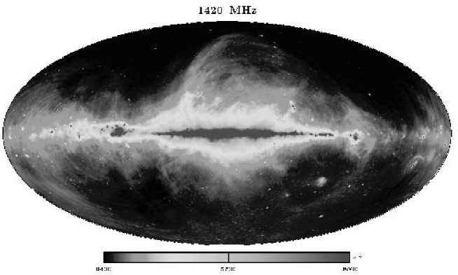
Figure 1: All-sky survey at 1.42 GHz combined from northern sky data observed with the Stockert 25-m telescope near Bonn/Germany (Reich 1982; Reich & Reich 1986) and southern sky observations observed with a 30-m dish at Villa Elisa/Argentina (Reich et al. (2001)).

2.2 Sky horn measurements

Continuum all-sky surveys receive their zero-level calibration by using low-resolution sky horn data. Their antenna diagrams are well known to enable a proper far-sidelobe correction. Reference loads at precisely known temperatures are required to find $\rm T_{sys}$. The all-sky surveys need to be convolved to the beam size of the sky horns, which are typically several degrees, to find the temperature offset. This way the 1.42 GHz survey (Fig. 1) was calibrated to an accuracy of 0.5 K $\rm T_{B}$. The 408 MHz survey by Haslam et al. (1982) has a zero-level accuracy of about 3 K $\rm T_{B}$. This accuracy is lower than the sensitivity (3 x r.m.s-noise) of both surveys of 0.05 K $\rm T_{B}$ and 2K $\rm T_{B}$, respectively.

The probably most famous sky horn observations are those by Penzias & Wilson (1965) leading to the discovery of the 3 K cosmic microwave background radiation. This led to the award of the Nobel Prize in 1978. Their absolute measurements revealed an isotropic sky component of 3.5 K, interpreted by Dicke et al. (1965) to originate from the CMB. This 4.08 GHz measurement of 3.5 K happened at a time, when ’relative’ measurements in the mK range were regularly made. This clearly reflects the technical challenges for these kind of measurements.

2.3 Adjusting surveys by TT-plots

Ground based surveys carried out at different frequencies with their zero-level adapted from sky horn measurements may be further adjusted relative to each other by using the so-called TT-plot method according to Turtle et al. (1962). This method was discussed in some detail by Reich et al. (2004). The surveys to be adjusted were convolved to a common angular resolution of 15^∘ and the TT-plots were performed for a strip in right ascension for declinations between 30^∘ and 45^∘, where no contamination from local structures like the giant loops is evident. As an example we show the TT-plot between the 408 MHz survey by Haslam et al. (1982) and the 1420 MHz survey by Reich (1982) in Fig. 2 (left panel) after a zero-level correction of -2.7 K for the 408 MHz survey. This correction is within its quoted zero-level error of 3 K. The mean of the fitted lines passes 0 K at both wavelengths. This result assumes the 1420 MHz survey to be correct, although the sky horn data are uncertain by 0.5 K. Using several pairs of surveys improves and constrains the corrections (see Reich et al. (2004) for details).

The WMAP total intensity all-sky surveys provide valuable high-frequency maps of Galactic emission and are of similar low-angular resolution compared to the ground based surveys up to 1.4 GHz. Unfortunately the WMAP total intensity maps have not yet set on an absolute zero-level. The three year’s release (Hinshaw et al. (2007)) at 22.8 GHz shows numerous small patches at high latitudes with temperatures below -100 $\mu$K, which is incorrect. We used the TT-plot technique to adjust the WMAP 22.8 GHz map in respect to 1420 MHz (see Fig. 2, right panel) and find an offset of 250$\pm 70~{}\mu$K. For the recent WMAP release of five years observations (Hinshaw et al., preprint), an offset of 260$\pm 70~{}\mu$K using the same method. This is quite a significant correction and has a clear effect on the spectral index between 1420 MHz and 22.8 GHz. The most frequent high-latitude temperature spectral indices increase from about -3.1 (without correction) to about -2.8, which is just slightly steeper (by about 0.1) compared to the spectra between 408 MHz and 1420 MHz.

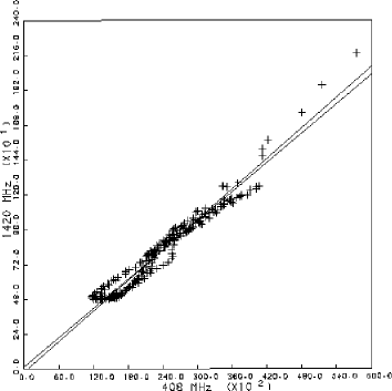
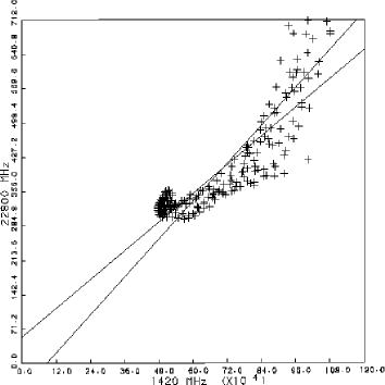
Figure 2: Left panel: TT-plot between the 408 MHz and 1420 MHz total intensity surveys leading to a zero-level correction of -2.7 K for the 408 MHz survey. Right panel: TT-plot between 1420 MHz and 22.8 GHz leading to an offset correction of the WMAP 3-yr survey by +250 $\mu$K.

Absolute sky measurements with high precision are needed to calibrate the WMAP total intensity maps. This is expected from ARCADE (Kogut et al. (2006)), a balloon-borne instrument designed to measure the absolute sky temperature between 3.3 GHz and 90 GHz in a number of channels. This exeriment will provide high-precision low-resolution data of Galactic emission.

2.4 Galactic plane surveys

Current Galactic plane surveys were carried out with large single-dish telescopes at arcmin angular resolution to resolve diffuse Galactic emission structures from individual sources like SNRs or HII-regions. Synthesis telescope surveys achieve even higher angular resolutions. These surveys use all-sky surveys to add the missing large-scale information and adjust their zero-level. This has been done using the total intensity northern sky 1.4 GHz survey (Fig. 1) to adjust 1.4 GHz Effelsberg total intensity surveys (Kallas & Reich 1980; Reich et al. (1990, 1997); Uyanıker et al. (1999)). These combined data at about 9’ angular resolution were used to calibrate the Canadian Galactic Plane Survey (CGPS) carried out with the synthesis telescope at DRAO/Penticton as described by Taylor et al. (2003), thus providing a survey including all structural information larger than 1’. Similarly the CGPS survey at 408 MHz uses the all-sky survey carried out by Haslam et al. (1982) with the Effelsberg, Parkes and Jodrell Bank telescopes at that frequency.

3 Calibration of polarization data

The scheme for ’relative’ and ’absolute’ zero-level calibration of polarization data, which means the calibration of the observed Stokes U and Q maps, in principle follows that of total intensity data: The absolute zero-level is required for all-sky maps and a relative zero-level setting is sufficient for polarized sources. The only ground-based all-sky polarization survey was made at 1.4 GHz by Wolleben et al. (2006) for the northern hemisphere using the DRAO 26-m telescope and by Testori et al. (2008) using one of the Villa Elisa 30-m telescopes for the southern sky, where the different calibration steps are discussed. The ’absolute zero-level’ of this polarization survey is adapted to 1.4 GHz measurements with the Dwingeloo 25-m telescope published by Brouw & Spoelstra (1976), where rotating dipoles were used allowing to separate sky emission from ground radiation contamination. The polarization intensity scale of these surveys, however, was adjusted by using smoothed polarization data from the Effelsberg or the Parkes telescopes, respectively. We show the combined all-sky 1.4 GHz polarization survey (Reich et al., in prep.) in Fig. 3.

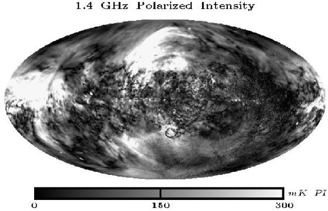
Figure 3: 1.4 GHz polarization all-sky survey combined from northern sky observations by Wolleben et al. (2006) and southern sky observations by Testori et al. (2008) at an absolute zero-level. The angular resolution of the survey is about 36’ and its sensitivity about 45 mK (3 x r.m.s-noise).

For the interpretation of Galactic polarization emerging from Faraday rotation in the interstellar medium, also the step of absolute zero-level calibration is required. Otherwise any interpretation becomes problematic, as it was discussed in some detail by Reich (2006). Polarization features emerging from Faraday rotation are in general not or very weakly related to total intensity sources or emission structures. The effect of zero-level calibration is different for polarized emission, because vectors are added, while for total intensities it is a scalar.

Polarized emission PI and polarization angle $\phi$ are calculated from the observed Stokes parameters U and Q, assumed to be corrected for all kinds of instrumental effects, by:

$$\rm PI^{2}~{}=~{}U^{2}~{}+~{}Q^{2}\quad and\quad\phi~{}=~{}0.5~{}atan(U/Q)$$ (2)

Adding missing components in $\rm U_{zero}$ and $\rm Q_{zero}$ gives:

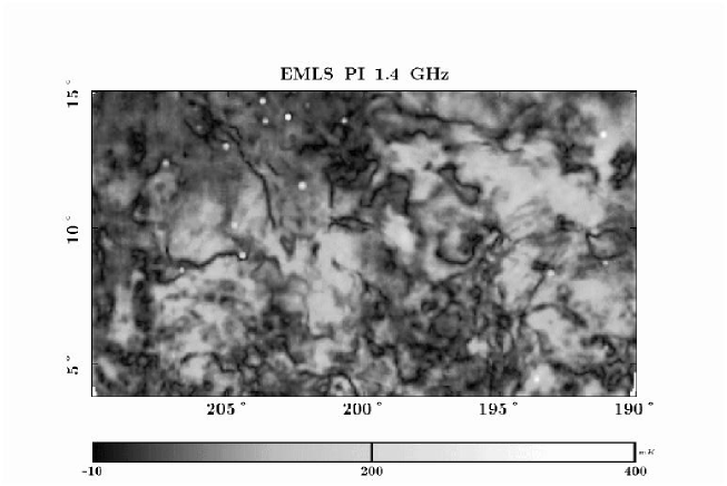
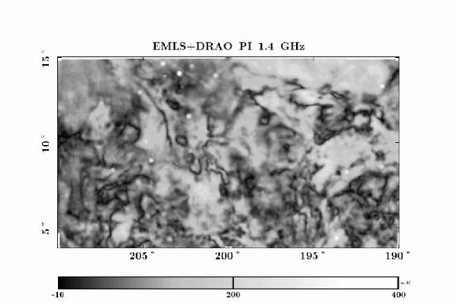
Figure 4: Example map showing polarized intensities from the 1.4 GHz ”Effelsberg Medium Latitude Survey” (Uyanıker et al. (1999)) with and without absolute zero-level adjustment. The upper panel shows the original Effelsberg map of polarized intensities. The lower panel shows the Effelsberg map with added large-scale components in U and Q exceeding the map size.

$$\rm PI_{abs}^{2}~{}=~{}(U+U_{zero})^{2}~{}+~{}(Q+Q_{zero})^{2}\quad\phi~{}=~{}0.5~{}atan((U+U_{zero})/(Q+Q_{zero}))$$ (3)

PI and $\phi$ depend on U(Q) and $\rm U_{zero}(Q_{zero})$ in a non-linear way. U(Q) and $\rm U_{zero}(Q_{zero})$ may have rather different levels and signs, that the inclusion of $\rm U_{zero}(Q_{zero})$ does not only change the level of PI, but also largely influences the morphology of the observed structures. This is demonstrated in Fig. 4, where 1.4 GHz polarized emission observed with the Effelsberg 100-m telescope is shown. The numerous small-scale polarization structures (’canals’ and ’rings’) have almost no counterpart in the very smooth total intensity map showing a smooth positive temperature gradient towards the Galactic plane and many compact extragalactic sources (see Uyanıker et al. (1999)). Fig. 4 shows the polarized emission as it was observed and after a correction for missing large-scale components provided by the northern sky polarization survey by Wolleben et al. (2006). The polarization level increases including large-scale components, but most remarkable is the change of morphology of the small-scale structures, which may change from absorption into emission structures and vice versa. Without the large-scale correction any physical interpretation or radiation transfer modelling of the observed features is strongly limited.

While the WMAP total intensity surveys need a zero-level correction as described above, this does not hold for the polarization data, where the maps are at a correct zero-level. WMAP observes difference signals from two feeds with about $140^{\circ}$ viewing angle difference (Bennett et al. (2003)). Other than for Stokes I, the Stokes parameter U and Q have no isotropic component.

3.1 Polarization surveys of the Galactic plane

With the availability of the 1.4 GHz all-sky polarization survey, Galactic plane surveys at 1.4 GHz can be properly calibrated as demonstrated in Fig. 4 for a section of the Effelsberg 1.4 GHz survey. The Effelsberg maps combined with the DRAO 26-m survey were then used to correct the 1.4 GHz polarized emission component of the CGPS, which results in a Galactic plane survey with 1’ angular resolution showing unprecedented details of the magnetized interstellar medium (Landecker et al., in prep.). This survey covers the Galactic plane in the longitude range $65^{\circ}\leq l\leq 175^{\circ}$ and latitudes between $-3.5^{\circ}\leq b\leq 5.5^{\circ}$. The filtering applied to the three surveys before merging the U and Q maps is shown in Fig. 5.

The WMAP polarization survey at 22.8 GHz (Page et al. (2007)) proves to be very valuable for the correction of high-resolution polarization data at a few GHz. Faraday rotation of the polarization angles at high latitudes and towards the anti-centre direction are small, that an extrapolation of the WMAP U and Q maps from 22.8 GHz towards lower frequencies is possible. This requires the correct spectral index for polarized emission, which should be close to that observed for total intensity synchrotron emission. For example a rotation measures (RM) of 50 rad $\rm m^{-2}$ causes a polarization angle rotation of about $10^{\circ}$ at $\lambda$6 cm. This technique was applied to the running Sino-German $\lambda$6 cm (4.8 GHz) polarization survey of the Galactic plane, which is carried out with the Urumqi 25-m telescope of NAOC/China. As described by Sun et al. (2007) this survey aims to cover the Galactic plane for latitudes between $\pm 5^{\circ}$ with an angular resolution of 9.5’ and a rms-sensitivity of 1.4(0.7) mK $\rm T_{B}$ for total (polarized) intensities. Measurements of an absolute polarization level of a few milli-Kelvin is a very ambitious task for a multi-purpose instrument like the Urumqi 25-m telescope and should be done with dedicated small instruments. The C-BASS project (Pearson & C-BASS collaboration 2007) might be able to provide this required information.

Sun et al. (2007) published the first survey map from the Urumqi $\lambda$6 cm survey and demonstrated the application of the WMAP zero-level correction for an area centered at Galactic longitude $125.5^{\circ}$. The zero-level offset extrapolated from the smoothed U and Q 22.8 GHz maps was found to be -0.3 mK $\rm T_{B}$ and 8.3 mK $\rm T_{B}$ for U and Q, respectively. The large value for Q indicates that the magnetic field runs almost parallel to the Galactic plane, as expected. The observed maps show a lot of diffuse polarized structures partly associated with SNRs, but also in the direction of some HII-regions, which act as Faraday screens and prove the presence of well-ordered magnetic fields of a few $\mu$G along the line-of-sight. Of particular interest is a large polarized structure in the field, G125.6-1.8, with a diameter of about 70’ showing no signature in total intensity nor in H$\alpha$-emission. This structure changes from a polarized emission structure as seen in the original Urumqi map into an absorption structure after WMAP calibration. The properties of this feature were modelled by Sun et al. (2007). For a size of 58 pc and a RM of 200 rad $\rm m^{-2}$ the calculated magnetic field strength exceeds 6.9 $\mu$G along the line-of-sight for an upper limit of the thermal electron density of 0.84 cm^-3 and assumed spherical symmetry. Such regular magnetic fields exceed the strength of the regular Galactic magnetic field, which is about 2$\mu$G in this area according to Han et al. (2006). The origin of these magnetic bubbles is not known, and it is also yet unclear how numerous they are and to what extent they influence the properties of the magnetized interstellar medium. Structures with such a high RM can not be studied at low frequencies, because small RM fluctuations cause depolarization across the observing beam. G125.6-1.8 is outstanding at $\lambda$6 cm, but remains undetected in the $\lambda$21 cm Galactic plane polarization survey by Landecker et al. (in prep.).

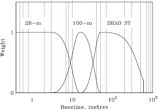
Figure 5: Weighting scheme of spatial structures applied to the three surveys as indicated (Landecker et al. in prep.). The combined maps in U and Q result in a Galactic plane survey, which is complete for all polarized structures larger than 1’ (see text).

3.2 Faraday screen observations

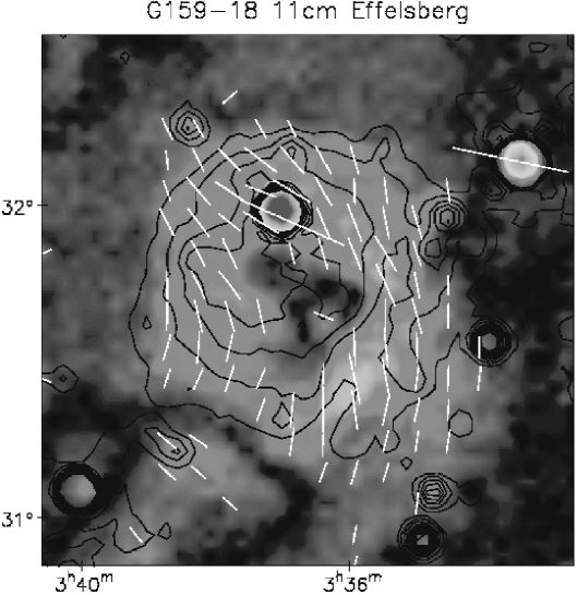
Figure 6: $\lambda$11 cm Effelsberg observations of the Perseus dust cloud G159.5-18.5 in total intensity (contours) and polarised intensity (greyscale and vectors). The linear polarization data indicate strong emission apparently originating from the thermal gas of G159.5-18.5. This is a clear indication that G159.5-18.5 acts as a Faraday screen rotating the polarization angle of background emission (see text).

Numerous Galactic polarized features were already discussed in the literature, but a number of them clearly suffer from insufficient calibration. As an example for a misinterpretation of that kind we discuss the case of the dust complex G159.5-18.5 in Perseus (Reich & Gao, in prep.). G159.5-18.5 is an extended source of about $1^{\circ}$ in size and very well studied at optical and infrared wavelengths, star light polarization and molecular line emission (Ridge et al. (2006) and references therein).

Recently G159.5-18.5 received particular attention, because it is one of the very few well established cases, where emission from spinning dust particles was clearly detected. Watson et al. (2005) presented observations made with the COSMOSOMAS telescope in the frequency range between 11 GHz and 17 GHz, which were combined with WMAP data at higher frequencies, showing a spectrum as expected for spinning dust emission, which is clearly in excess over the weak thermal emission. Battistelli et al. (2006) presented 11 GHz polarization observations with the COSMOSOMAS telescope of a large area in Perseus and detected faint polarized emission of 3.4% +1.5%/-1.9% from G159.5-18.5, which they interpreted as polarized emission emerging from spinning dust grains, which would be the first detection of that kind. However, the polarization data are on a relative zero-level in U and Q.

Watson et al. (2005) extracted information of the thermal emission component of G159.5-18.5 from existing ground based all-sky surveys. Recent pointed observations with the Effelsberg 100-m telescope at $\lambda$11 cm and the Urumqi 25-m telescope at $\lambda$6 cm with higher quality clearly confirm the existence of optically thin thermal gas in G159.5-18.5 with a flux density of about 3.8 Jy, more than four times below the flux density of spinning dust seen at COSMOSOMAS wavelengths. Surprisingly strong polarized emission was observed at $\lambda$11 cm (Fig. 6) and $\lambda$6 cm, which is not expected to originate from thermal gas. Spinning dust plays no role at $\lambda$11 cm wavelength, that the only valid interpretation is that G159.5-18.5 acts as a Faraday screen hosting a strong regular magnetic field along the line-of-sight. The Faraday screen rotates the background polarized emission of G159.5-18.5, which then adds to foreground polarization in a different way than in the area outside of G159.5-18.5. In fact, correcting the Battistelli et al. (2006) polarization data of G159.5-18.5 for missing large-scale emission as observed by WMAP reduces the polarized emission signal below that of its surroundings.

The Faraday screen model as discussed by Reich & Gao (in prep.) fits all available polarization observations with a RM of the order of 190 rad m^-2 implying a line-of-sight magnetic field of about 10 $\mu$G.

4 Conclusions

We have discussed calibration methods being applied to all-sky and Galactic plane continuum surveys in total intensity and linear polarization. The interpretation of polarized emission emerging from Faraday rotation effects in the interstellar medium requires special attention, in paparticularn absolute zero-level setting is essential.