Optical Bragg, atom Bragg and cavity QED detections of quantum phases and excitation spectra of ultracold atoms in bipartite and frustrated optical lattices

Abstract

Ultracold atoms loaded on optical lattices can provide unprecedented experimental systems for the quantum simulations and manipulations of many quantum phases and quantum phase transitions between these phases. However, so far, how to detect these quantum phases and phase transitions effectively remains an outstanding challenge. In this paper, we will develop a systematic and unified theory of using the optical Bragg scattering, atomic Bragg scattering or cavity QED to detect the ground state and the excitation spectrum of many quantum phases of interacting bosons loaded in bipartite and frustrated optical lattices. The physical measurable quantities of the three experiments are the light scattering cross sections, the atom scattered clouds and the cavity leaking photons respectively. We show that the two photon Raman transition processes in the three detection methods not only couple to the density order parameter, but also the valence bond order parameter due to the hopping of the bosons on the lattice. This valence bond order coupling is very sensitive to any superfluid order or any Valence bond (VB ) order in the quantum phases to be probed. These quantum phases include not only the well known superfluid and Mott insulating phases, but also other important phases such as various kinds of charge density waves (CDW), valence bond solids (VBS), CDW-VBS phases with both CDW and VBS orders unique to frustrated lattices, and also various kinds of supersolids. We analyze respectively the experimental conditions of the three detection methods to probe these various quantum phases and their corresponding excitation spectra. We also address the effects of a finite temperature and a harmonic trap. We contrast the three scattering methods with recent in situ measurement inside a harmonic trap and argue that the two kinds of measurements are complementary to each other. The combination of both kinds of detection methods could be used to match the combination of Scanning tunneling microscopy (STM), the Angle Resolved Photo Emission spectroscopy ( ARPES ) and neutron scattering in condensed matter systems, therefore achieve the putative goals of quantum simulations

I Introduction

Various kinds of strongly correlated quantum phases of matter may have wide applications in quantum information processing, storage and communications manybody . It was widely believed and also partially established that due to the tremendous tunability of all the parameters in this system, ultracold atoms loaded on optical lattices (OL) can provide an unprecedented experimental systems for the quantum simulations and manipulations of these quantum phases and quantum phase transitions between these phases. For example, Mott and superfluid phases boson may have been successfully simulated and manipulated by ultra-cold atoms loaded in a cubic optical lattice bloch . However, there are still at least two outstanding problems remaining. The first is to how to realize many important quantum phases manybody . The second is that assuming the favorable conditions to realize these quantum phases are indeed achieved in experiments, how to detect them without ambiguities. In this paper, we will address the second question.

Because these ultra-cold atoms are charge neutral, so in contrast to many condensed matter systems, they can not be manipulated electrically or magnetically, so the experimental ways to detect these quantum phases of cold atoms are rather limited. The earliest detection method is through the so called time of flight measurement manybody ; bloch which simply opens the trap and turn off the optical lattice and let the trapped atoms expand and interfere, then take the image. This kind of measurement is destructive and may not be used to detect the ground state and excitation spectrum of quantum phases in optical lattices. There are also other detection methods such as the Optical Bragg scattering in Fig.1a and the atom Bragg scattering in Fig.1b. The Optical Bragg scattering (Fig.1a) has been used previously to study periodic lattice structures of cold atoms loaded on optical lattices braggsingle . It was also proposed as an effective method for the thermometry of fermions in an optical lattice braggthermal . Recently, it was argued that it can be used to detect the putative anti-ferromagnetic ground state of fermions in OL braggafm . There are also very recent optical Bragg scattering experimental data from a Mott state, a BEC and some artificial AF state blochlight . The atom Bragg diffraction in Fig.1b ( also called ”atom Bragg spectroscopy ” ) is based on stimulated matter waves scattering by two incident laser pulses braggbog ; braggeng , then take images through the time of flight measurements. There are also two kinds of ”atom Bragg spectroscopies ”. The momentum braggbog transfer Bragg spectroscopy was used to detect the Bogoliubov mode inside an BEC condensate. The energy transfer braggeng Bragg spectroscopy was used to detect the Mott gap in a Mott state in an optical lattice. The photon and atom Bragg diffractions are two complementary experimental detection methods. During the last several years, there have been extensive of experimental and theoretical research combining cavity QED and cold atoms. For example, several experiments qedbec1 ; qedbec2 successfully achieved the strong coupling of a BEC of $N\sim 10^{5}$ ${}^{87}Rb$ atoms to the photons inside an ultrahigh-finesse optical cavity. The super-radiant phase phased was realized in a recent experiments orbital using BEC and also in a previous experiment using thermal atoms orbitalt where the effective two ”atomic” levels are the two momentum states of the cold atoms in the optical lattice formed by the cavity field and the off-resonant transverse pumping Laser. Since the first experimental observation of the bi-stabilities of BEC atoms at very low photon numbers inside a cavity qedbecoff , there have been very active theoretical studies on the bi- or multi-instabilities of BEC spinors spinor , spinless fermions fermion or BEC with a spin-orbit coupling spinorbit inside a cavity. It was also preliminarily proposed that the cavity photons may be used to non-destructively detect superfluid and Mott phases of ultra-cold atoms in optical lattices. ( The quantitative theory will be developed in Sec.VIII and the Appendix D ) off1 ; off2 .

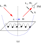
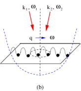
Figure 1: Optical (a) and atom (b) Bragg scattering of cold atoms moving in 2 dimensional optical lattices. The $\vec{q}=\vec{k}_{1}-\vec{k}_{2}$ and $\omega=\omega_{1}-\omega_{2}$ are momentum and energy transfer from the laser beams to the cold atoms respectively. Tilting and rotating the incident beam(s) around the dashed line can probe the ground state and the excitation spectrum of the whole 2d optical lattice.

In this paper, we will explore the applicabilities of both photon Bragg diffraction and atom Bragg diffraction to detect several important quantum phases in both bipartite and frustrated lattices. We will also discuss in detail the possibility that the cavity QED can be used as a possible new detection method. The physical measurable quantities of the three experiments are the light scattering cross sections, the atom scattered clouds and the cavity leaking photons respectively. All these experimental measurable quantities are determined by the density-density and bond-bond correlation functions. We will develop a systematic and unified theory of using the optical Bragg scattering, atomic Bragg scattering or cavity QED to detect the nature of quantum phases such as both the ground state and the excitation spectrum above the ground state of interacting bosons loaded in optical lattices.

The Extended Boson Hubbard Model (EBHM) with various kinds of interactions, on all kinds of lattices and at different filling factors is described by the following Hamiltonian boson ; bloch ; gan ; square ; sca ; frusqmc ; pq1 ; mob ; bipart ; frus ; honey :

$$H_{BH} = -t\sum_{\langle ij\rangle}(b^{\dagger}_{i}b_{j}+h.c.)-\mu\sum_{i}n_{i}+\frac{U}{2}\sum_{i}n_{i}(n_{i}-1)$$ (1)

$$+ V_{1}\sum_{<ij>}n_{i}n_{j}+V_{2}\sum_{\langle ik\rangle}n_{i}n_{k}+\cdots$$

where $n_{i}=b^{\dagger}_{i}b_{i}$ is the boson density, $t$ is the nearest neighbor hopping which can be tuned by the depth of the optical lattice potential, the $U,V_{1},V_{2}$ are onsite, nearest neighbor (nn) and next nearest neighbor (nnn) interactions respectively, the $\cdots$ may include further neighbor interactions, dipole-dipole interaction $V=\frac{p^{2}}{|\vec{r}_{i}-\vec{r}_{j}|^{3}}$ and possible ring-exchange interactions. The filling factor $n=N_{a}/N$ where $N_{a}$ is the number of atoms and $N$ is the number of lattice sites. The on-site interaction $U$ can be tuned by the Feshbach resonance boson . There are many possible ways to generate longer range interaction $V_{1},V_{2},....$ of ultra-cold atoms loaded in optical lattices. Being magnetically or electrically polarized, the ${}^{52}Cr$ atoms cromium or polar fermionic molecules junpolar ${}^{40}K+^{87}Rb$ ( or bosonic molecules ${}^{39}K+^{87}Rb$ ) interact with each other via long-rang anisotropic dipole-dipole interactions. Loading the ${}^{52}Cr$ or the polar bosonic molecules on a 2d optical lattice with the dipole moments perpendicular to the trapping plane can be mapped to Eqn.1 with long-range repulsive interactions $\sim p^{2}/r^{3}$ where $p$ is the dipole moment. Possible techniques to generate long-range interactions in a gas of ground state alkali atoms by weakly admixing excited Rydberg states with laser light was proposed in mixture . The generation of the ring exchange interaction has been discussed in qs .

Various kinds of bipartite and frustrated optical lattices can be realized by suitably choosing the geometry of the laser beams generating the optical lattices. For example, using three coplanar beams of equal intensity having the three vectors making a $120^{\circ}$ angle with each other, the potential wells have their minima in a honeycomb or a triangular lattice honeylattice . Four beams travel along the three fold symmetry axes of a regular tetrahedron, the potential wells have their minima in a body-centered-cubic lattice honeylattice . The authors in kalattice proposed to create a kagome optical lattice using superlattice techniques. It was known that cold atoms in a frustrated lattice show completely different behaviors than in a bipartite lattice. Some of the important phases with long range interactions in bipartite lattices are studied in details in square ; squaresoft ; frusqmc ; honey ; pq1 ; mob ; bipart ; frus and listed in Fig.2 and 3. Some quantum phases in frustrated lattices are studied in gan ; frus and will be briefly reviewed in the appendix A.

In this paper, we explicitly show that the two photon Raman transition processes shown in Fig.4 in the optical Bragg scattering, atomic Bragg scattering or cavity QED ( with the classical scattered light in Fig.1a replaced by the quantum cavity photon in Fig.11 ) not only couple to the density order parameter, but also the valence bond order parameter due to the hopping of the bosons on the lattice. This kinetic energy coupling is extremely sensitive to any superfluid order or any Valence bond (VB ) order which can be considered as a local superfluid order on a local bond at corresponding ordering wavevectors. By tuning the incident angle in the Fig.1a, the angle between the two laser lights in Fig.1b or the incident light and the cavity axis in Fig.11a, one can detect both the ground state and the excitation spectrum by measuring the light scattering cross sections, the atom scattered clouds and the leaking cavity photon numbers respectively. The static structure function can detect not only the well known superfluid and Mott insulating phases, but also other interesting phases such as charge density wave (CDW), both dimer and plaquette valence bond solids (VBS), even some CDW-VBS phase unique in frustrated lattices at commensurate fillings gan ; square ; frusqmc ; pq1 ; mob ; bipart ; frus ; honey . It can also detect the corresponding CDW supersolids and VB supersolids at in-commensurate fillings in both bipartite and frustrated lattices. Furthermore, the dynamic structure function can detect the excitation spectrum and the corresponding spectral weights in all these quantum phases.

Recently, there are very impressive advances in probing individual atoms without and with optical lattices using electron and optical microscopy local0 ; local1 ; insitu0 ; insitu1 . It is a direct in situ measurements on individual density and density fluctuations. For example, the superfluid phase and the Mott phase in optical lattices studied by the earliest time of flight measurements in bloch are probed by the spatially resolved, in situ imagings. As argued in Sec. IX, the in situ measurement is an effective measurement of local density and density fluctuations. Under the local density approximation (LDA), these in situ imagings can be used to extract the temperature of the system and test the scaling relations of thermodynamic quantities across classical and quantum phase transitions trapthe0 ; trapthe1 , but so far, it may not be used to test the dynamic density-density or bond-bond scaling relations which are non-local in the space and time, their peak positions lead to the excitation spectra of the corresponding quantum phases ( See Fig.8 ). These dynamic correlation function can be precisely measured by the three scattering methods to be studied in this paper. However, all the three scattering methods involve large number of atoms in the system, so it is a momentum space probes, so it may not resolve the local information. So the scattering detection methods and the in situ measurements are complementary and dual to each other. Both kinds of measurement involve density or bond and their correlations, but the former focus in momentum space, the latter in the real space, similar to the relation between the ARPES versus STM in high temperature superconductors hightc . In Sec.IX, we will compare both kinds of methods in some details.

The rest of the paper is organized as the follows. In Sec.II, just from symmetry breaking points of view, we study several very general and important properties of density-density, bond-bond correlation functions and their finite size scaling properties inside a flat trap flattrap . In Sec. III, we study the off-resonant light scattering from the two level atoms hopping in an optical lattice and find the off-resonant light beams not only couple to the density, but also the kinetic energy of the cold atoms hopping on a optical lattice. We also estimate the relative strengths of the two couplings by using the harmonic approximation boson . We show that the light scattering cross section is the sum of the density-density and bond-bond correlation function with the corresponding form factors. In Sec.IV, we study the density-density correlation function in the superfluid, Mott and quantum critical regime at integer filling case from both the boson action and its dual vortex action. All the previous work seem focused on the order parameter correlation functions instead of the density-density ones which are measured by the three experimental detection methods. In Sec. V, we study the elastic scattering cross section in a CDW to detect the ground state, also in-elastic scattering cross section to detect the excitation spectrum and its scaling form near the second order transition from the CDW and CDW supersolid. In Sec. VI, we study the elastic scattering cross section in a VBS to detect the ground state, also in-elastic scattering cross section to detect its excitation spectrum and its scaling form near the second order transition from the VBS and VBS supersolid. In Sec. VII, we extend our discussions to frustrated lattices and stress several new features in the density-density and bond-bond correlation functions unique to frustrated lattices. Then we apply the formalism to study the light scattering cross sections from the X-CDW, VBS and CDW-VBS phases in a triangular lattice. In Sec.VIII, we propose to use cavity QED as an effective detection method. Phase sensitive homodyne measurement and the Florescence spectrum measurement can be used to detect the ground state and excitation spectrum of various quantum phases. This possible cavity enhanced off-resonant light scattering detection method should be complementary to the light scattering and atom Bragg scattering discussed in the previous sections. In the Sec. IX, we discuss quantum phases and quantum phase transitions inside a harmonic trap. We classify the necessary conditions for the local density approximation ( LDA ) to hold and give the scaling forms for the static and equal time density-density ( or bond-bond ) correlation functions under the LDA. We compare the scattering detection methods with the in situ local measurements. We also point out the possibility to experimentally observe a stable ring-structure supersolid of dipolar bosons inside a harmonic trap. In the final Sec.X, we contrast the three scattering experiments, also the in situ local measurements, discuss their strengths and weaknesses in detecting all these quantum phases and summarize our results. In the appendix A, we will review several important phases in both bipartite and frustrated lattices. We also stress a recently discovered new phase which has both CDW and VBS order called CDW-VBS phase in the triangular lattice. This kind of CDW-VBS phase is unique and quite common to frustrated lattices. In the appendix B, we discuss light Bragg scattering experiment and a possible quantum beat measurement to measure small energy differences in inelastic light Bragg scattering experiment. In the appendix C, we analyze both momentum and energy atom Bragg scattering experiments. In the Appendix D, we point out some mistakes in the previous work off1 and show that the light scattering cross section or cavity QED scattering at the classical diffraction minimum $\vec{q}=(\pi,\pi)$ may be an effective measurement of the superfluid density $\rho_{s}$. A short report on some results of this paper already appeared in braggprl . In the following, we just take 2d optical lattices as examples. The 1d and 3d cases can be similarly discussed .

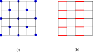
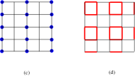
Figure 2: Several insulating states at filling factor $f=1/2$ in a square lattice. (a) The charge density wave (CDW) phase with ordering wavevector $\vec{Q}_{n}=(\pi,\pi)$. (b) valence bond solid (VBS) phases with ordering wavevector $\vec{Q}_{K}=(\pi,0)$ where the kinetic energy $\langle K_{ij}\rangle=\langle b^{\dagger}_{i}b_{j}+h.c.\rangle$ takes a non-zero constant $K$ in the two sites connected with a dimer, but $0$ in the two sites without a dimer. (c) Stripe CDW order at $\vec{Q}_{n}=(\pi,0)$ and (d) Plaquette VBS order at $\vec{Q}_{K1}=(\pi,0),\vec{Q}_{K2}=(0,\pi)$. See Refs.gan ; pq1 ; mob ; bipart ; frus .

II Density-density and bond-bond correlation functions in a bipartite lattice

In this section, from symmetry breaking point of view, we will study several important properties of the density-density correlation functions and the bond-bond correlation functions in these quantum phases in a bipartite lattice respectively. The counterparts in a frustrated lattice will be discussed in Sec.VII. The results achieved should also be useful to Quantum Monte Carlo simulations square ; squaresoft ; honey on the extended boson Hubbard model in Eqn.1 in a finite $N=L\times L$ lattice.

II.1 Density-Density correlation function

In view of the possible CDW ordering at $\vec{q}=\vec{Q}_{N}$, one can decompose the density at site $i$ as

$$N_{i}=n_{i}+(-1)^{i}m_{i}$$ (2)

where $i=x$ for the $\vec{Q}_{N}=(\pi,0)$ stripe CDW in Fig.2c and $i=x+y$ for the $\vec{Q}_{N}=(\pi,\pi)$ CDW in Fig.2c. Then the density-density correlation function is defined as:

$$S_{N}(\vec{q},t)=\frac{1}{N^{2}}\sum_{i,j}e^{-i\vec{k}\cdot(\vec{r}_{i}-\vec{r}_{j})}\langle N_{i}(t)N_{j}(0)\rangle$$ (3)

By substituting the decomposition of $N_{i}$ into the above Eqn. we can get:

$$S_{N}(\vec{q},t) = \frac{1}{N}\sum_{i}e^{-i\vec{q}\cdot\vec{r}_{i}}\langle n(i,t)n(0,0)\rangle_{C}+n^{2}\delta_{\vec{q},0}$$ (4)

$$+ \frac{1}{N}\sum_{i}e^{-i(\vec{q}-\vec{Q}_{N})\cdot\vec{r}_{i}}\langle m(i,t)m(0,0)\rangle_{C}$$

$$+ m^{2}\delta_{\vec{q},\vec{Q}_{N}}$$

where we have used the translational invariance to get rid of one summation, $\langle n_{i}(t)n_{j}(0)\rangle_{C}=\langle n_{i}(t)n_{j}(0)\rangle-n^{2}$ and $\langle m_{i}(t)m_{j}(0)\rangle_{C}=\langle m_{i}(t)m_{j}(0)\rangle-m^{2}$ are connected Green functions.

Its Fourier transform leads to the dynamic structure function:

$$S_{N}(\vec{q},\omega) = \int dte^{-i\omega t}S_{N}(\vec{q},t)$$ (5)

$$= n^{2}\delta_{\vec{q},0}\delta(\omega)+\frac{1}{N}S^{inel}_{n}(\vec{q},\omega)$$

$$+ m^{2}\delta_{\vec{q},\vec{Q}_{N}}\delta(\omega)+\frac{1}{N}S^{inel}_{m}(\vec{q},\omega)$$

where the first and the third $\delta(\omega)$ terms denote the elastic scattering at $\vec{q}=0$ and $\vec{q}=\vec{Q}_{N}$ respectively $S^{el}_{n}\delta(\omega)=n^{2}\delta_{\vec{q},0}\delta(\omega),S^{el}_{m}\delta(\omega)=m^{2}\delta_{\vec{q},\vec{Q}_{N}}\delta(\omega)$, the second and the fourth terms denote the inelastic scattering near $\vec{q}=0$ and $\vec{q}=\vec{Q}_{N}$ respectively.

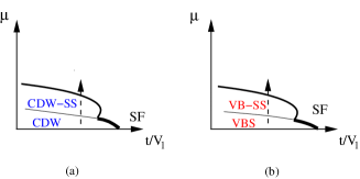
Figure 3: Zero temperature Phase diagram of the boson Hubbard model with nearest neighbor interaction $V_{1}$ near half filling in a bipartite lattice bipart . The labels of the axes are given in Eqn.1. (a) Ising limit. (b) Easy-Plane limit. See also Fig. 9 for the finite temperature phase diagram and Fig.13 for the phases inside a trap.

The equal time density-density correlation function is:

$$S_{N}(\vec{q},t=0) = \frac{1}{N}\sum_{i}e^{-i\vec{q}\cdot\vec{r}_{i}}\langle n(i,0)n(0,0)\rangle_{C}+n^{2}\delta_{\vec{q},0}$$ (6)

$$+ \frac{1}{N}\sum_{i}e^{-i(\vec{q}-\vec{Q}_{N})\cdot\vec{r}_{i}}\langle m(i,0)m(0,0)\rangle_{C}$$

$$+ m^{2}\delta_{\vec{q},\vec{Q}_{N}}$$

From $S_{N}(\vec{q},t=0)=\int\frac{d\omega}{2\pi}S_{N}(\vec{q},\omega)$, we can write the equal-time correlation function as the sum of the elastic one and the in-elastic one:

$$S_{N}(\vec{q},t=0)=S^{el}_{n}+\frac{1}{N}S^{inel}_{n}(\vec{q})+S^{el}_{m}+\frac{1}{N}S^{inel}_{m}(\vec{q})$$ (7)

where $S^{el}_{n}=n^{2}\delta_{\vec{q},0},S^{el}_{m}=m^{2}\delta_{\vec{q},\vec{Q}_{N}}$ and $S^{inel}_{n}(\vec{q})=\int\frac{d\omega}{2\pi}S^{inel}_{n}(\vec{q},\omega),S^{inel}_{m}(\vec{q})=\int\frac{d\omega}{2\pi}S^{inel}_{m}(\vec{q},\omega)$.

In the following, we discuss the density-density correlation functions in the superfluid, CDW and CDW supersolid respectively.

(a) Superfluid state near $\vec{q}=0$.

In the superfluid state, the first term in Eqn.4 stands for the gapless superfluid mode near $\vec{q}=0$. Taking the results from Ref.ssorder ; sforder , we have:

$$S^{SF}_{n}(\vec{q},\omega)=\langle\delta n(-\vec{q},-\omega_{n})\delta n(\vec{q},\omega_{n})\rangle=\frac{\rho_{s}q^{2}}{\omega^{2}_{n}+v^{2}q^{2}}$$ (8)

where $v^{2}=\rho_{s}/\kappa$ is the superfluid phonon velocity, the $\rho_{s}$ is the superfluid density and the $\kappa$ is the compressibility. Indeed

$$\kappa_{SF}=S^{SF}_{n}(\vec{q}\rightarrow 0,\omega=0)=\rho_{s}/v^{2}$$ (9)

as it should be. Note that the compressibility can also be directly measured by the in situ method insitu0 ; insitu1 ( see Sec.IX for details ). From the analytical continuation $i\omega_{n}\rightarrow\omega+i\delta$ and taking the imaginary part, we can identify the dynamic structure factor:

$$S^{>}_{n}(\vec{q},\omega)=S_{n}(q)\delta(\omega-vq),~{}~{}~{}S_{n}(q)=\rho_{s}q\pi/2v$$ (10)

where the $S_{n}(q)$ is the equal time density-density correlation function near $q=0$ shown in Fig.8a1.

The second term near $\vec{q}=\vec{Q}_{N}$ in Eqn.4 comes from the roton contribution near $\vec{q}=\vec{Q}_{N}$ in Fig.8a1. The dispersion near $\vec{q}=\vec{Q}_{N}$ can be taken as $\omega(q)\sim\Delta_{r}+\frac{(\vec{q}-\vec{Q}_{N})^{2}}{2m_{r}}$ where $\Delta_{r}>0$ is the roton gap. There is no CDW order yet, so $m=0$ in the Eqn.4. However, as one approaches the CDW from the SF in Fig.3a, there is a first order transition into the CDW driven by the collapse of the roton gap $\Delta_{r}$.

(b) CDW state near $\vec{q}=\vec{Q}_{N}$.

In the CDW state, the $nn$ correlator near $\vec{q}=0$ in Eqn.4 is very small, so can be dropped safely, so one only need to focus on the $mm$ correlator near $\vec{q}=\vec{Q}_{N}$. The discrete lattice symmetry was broken due to the non-uniform density distribution, so $m\neq 0$, there is also a gap $\Delta_{CDW}$ in the CDW state, so the connected equal time correlation function decays exponentially in the CDW state:

$$\langle m_{i}(0)m_{j}(0)\rangle_{C}\sim e^{-|\vec{r}_{i}-\vec{r}_{j}|/\xi_{CDW}}$$ (11)

where $\xi_{CDW}\sim 1/\Delta_{CDW}$ is the correlation length in the CDW. So the fluctuation part in Eqn.6 is only at the order of $\sim 1/N$, we conclude:

$$S_{N}(\vec{Q}_{N},t=0)=m^{2}+\frac{1}{N}S^{inel}_{m}(\vec{q}=\vec{Q}_{N})=m^{2}+O(1/N)$$ (12)

Here we can see that the equal time structure factor is the sum of the elastic scattering $S^{el}_{m}=m^{2}$ plus a $1/N$ in-elastic background.

For $\vec{q}\neq\vec{Q}_{N}$, but close to $\vec{Q}_{N}$, then we find

$$S_{N}(\vec{q},t)\sim\frac{1}{N}\sum_{i}e^{-i(\vec{q}-\vec{Q}_{N})\cdot\vec{r}_{i}}\langle m(i,t)m(0,0)\rangle_{C}$$ (13)

where one can extract the excitation spectrum and spectral weight of the CDW near $\vec{q}\neq\vec{Q}_{N}$ shown in Fig.8c1. In fact, the excitation spectrum around $\vec{k}-\vec{Q}_{N}=\vec{q}$ can also be extracted from the Feynman relation:

$$\omega_{CDW}(\vec{q})=\frac{\int^{\infty}_{-\infty}d\omega\omega S_{N}(\vec{q},\omega)}{\int^{\infty}_{-\infty}d\omega S_{N}(\vec{q},\omega)}$$ (14)

which holds at $\vec{q}\rightarrow 0$, but not at $\vec{q}=0$. The $f$-sum rule $\int^{\infty}_{-\infty}d\omega\omega S_{N}(\vec{q},\omega)=\langle[[n(\vec{q}),H],n(-\vec{q})]\rangle$ at $d=2$ gives:

$$\int^{\infty}_{-\infty}d\omega\omega S_{N}(\vec{q},\omega)=-2t\sum_{\vec{k}}[(\cos q_{x}-1)\cos k_{x}$$

$$+(\cos q_{y}-1)\cos k_{y}]\langle\Psi_{0}|b^{\dagger}_{\vec{k}}b_{\vec{k}}|\Psi_{0}\rangle~{}~{}~{}~{}~{}~{}~{}~{}~{}~{}~{}$$ (15)

where the $|\Psi_{0}\rangle$ is the ground state wavefunction.

The $d=1$ version of this sum rule was used to extract the excitation spectra by QMC in both the SF and the CDW state in Ref.sca . Note that at $d=1$, the SF to the CDW transition along the horizontal axis in Fig.3a is in the Kosterlitz-Thouless (KT) transition universality class instead of first order transition in $d=2$ and $d=3$. We expect that the SF to the CDW-SS transition in Fig.3a is also in the KT transition universality class.

(c) CDW Supersolid state

In this case, the first term near $\vec{q}=0$ in Eqn.4 stands for the gapless superfluid mode as given by Eqn.8 and shown in the lower branch in Fig.8b1.

The static order at $\vec{q}=\vec{Q}_{N}$ is given by Eqn.12 and the dynamic structure factor close to $\vec{Q}_{N}$ in the upper branch in Fig.8b1 is given by Eqn.13 respectively.

II.2 The bond-bond correlation function

Inside a VBS state with a ordering wavevector $\vec{Q}_{K}$, similar to Eqn.2, one can write the kinetic energy at a given bond $i,\alpha,\alpha=\hat{x},\hat{y}$ as

$$D_{i,\alpha}=B_{i,\alpha}+e^{i\vec{Q}_{K}\cdot\vec{r}_{i}}K_{i,\alpha}$$ (16)

For example, for the $\vec{Q}_{K}=(\pi,0)$ VBS state, Eqn.16 becomes:

$$D_{ix} = B_{ix}+(-1)^{i_{x}}K_{ix}$$

$$D_{iy} = B_{iy}=B_{ix}$$ (17)

Then the bond-bond correlation function is defined as:

$$S_{D\alpha}(\vec{q},t)=\frac{1}{N^{2}}\sum_{i,j}e^{-i\vec{k}\cdot(\vec{r}_{i}-\vec{r}_{j})}\langle D_{i\alpha}(t)D_{j\alpha}(0)\rangle$$ (18)

By substituting the decomposition Eqn.16 into the above Eqn. we can get:

$$S_{D\alpha}(\vec{q},t) = \frac{1}{N}\sum_{i}e^{-i\vec{q}\cdot\vec{r}_{i}}\langle B_{\alpha}(i,t)B_{\alpha}(0,0)\rangle_{C}+B^{2}\delta_{\vec{q},0}$$ (19)

$$+ \frac{1}{N}\sum_{i}e^{-i(\vec{q}-\vec{Q}_{K})\cdot\vec{r}_{i}}\langle K_{\alpha}(i,t)K_{\alpha}(0,0)\rangle_{C}$$

$$+ K^{2}\delta_{\vec{q},\vec{Q}_{K}}$$

where the $\langle B_{\alpha}(i,t)B_{\alpha}(0,0)\rangle_{C}=\langle B_{\alpha}(i,t)B_{\alpha}(0,0)\rangle-B^{2}$ and $\langle K_{\alpha}(i,t)K_{\alpha}(0,0)\rangle_{C}=\langle K_{\alpha}(i,t)K_{\alpha}(0,0)\rangle-K^{2}$ are connected Green functions.

In a VBS or a VBS superfluid state, the density is uniform, then the Eqn.4 should be replaced by:

$$S_{N}(\vec{q},t)=\frac{1}{N}\sum_{i}e^{-i\vec{q}\cdot\vec{r}_{i}}\langle n(i,t)n(0,0)\rangle_{C}+n^{2}\delta_{\vec{q},0}$$ (20)

where there is no staggered component $m$.

Inside a VBS state with a ordering wavevector $\vec{Q}_{K}$, there is a big CDW gap in the connected density-density correlation function in Eqn.20. Obviously, this CDW gap is much larger than the VBS gap introduced below Eqn.22. Furthermore, $S_{N}(\vec{Q}_{K},0)=\frac{1}{N}\sum_{i}e^{-i\vec{Q}_{K}\cdot\vec{r}_{i}}\langle n(i,0)n(0,0)\rangle_{C}$ is a smearing of a very small density fluctuation on a lattice scale, so it contributes to a very small background which is completely negligible compared to the VBS fluctuations near $\vec{Q}_{K}$ to be discussed in the following. ( Note that inside a superfluid, it may still be appreciable even at the classical diffraction minimum $\vec{q}=(\pi,\pi)$ as to be shown in the Appendix B ).

(a) Superfluid near $\vec{q}=0$.

The gapless superfluid mode near $\vec{q}=0$ in Eqn.20 is still given by Eqn.8, but there is no peak near $\vec{q}=\vec{Q}_{K}$ in Eqn.20. Instead, there is a peak near $\vec{q}=\vec{Q}_{K}$ in the bond-bond correlation function in Eqn.21. The excitation spectrum near $\vec{q}=\vec{Q}_{K}$ can be taken as $\omega_{v}(q)\sim\Delta_{rv}+\frac{(\vec{q}-\vec{Q}_{K})^{2}}{2m_{rv}}$ where $\Delta_{rv}>0$ is the ” valence bond roton” gap. There is no VBS order yet, so $K=0$ in the Eqn.21. However, as one approaches the VBS from the SF in Fig.3b, there maybe a first order transition into the VBS driven by the collapse of the gap $\Delta_{rv}$.

(b) VBS state

The lattice symmetry was broken by the non-uniform kinetic energy, so $K\neq 0$. One can neglect the very small $BB$ fluctuations near $\vec{q}=0$ in Eqn.19. Then Eqn.19 can be simplified to:

$$S_{K\alpha}(\vec{q},t) = \frac{1}{N}\sum_{i}e^{-i(\vec{q}-\vec{Q}_{K})\cdot\vec{r}_{i}}\langle K_{\alpha}(i,t)K_{\alpha}(0,0)\rangle_{C}$$ (21)

$$+ K^{2}\delta_{\vec{q},\vec{Q}_{K}}$$

where $\vec{Q}_{K}=(\pi,0)$ is the ordering wavevector for the VBS.

The equal time bond-bond correlation function is:

$$S_{K\alpha}(\vec{q},t=0) = \frac{1}{N}\sum_{i}e^{-i(\vec{q}-\vec{Q}_{K})\cdot\vec{r}_{i}}\langle K_{\alpha}(i,0)K_{\alpha}(0,0)\rangle_{C}$$ (22)

$$+ K^{2}\delta_{\vec{q},\vec{Q}_{K}}$$

Inside the VBS, there is also a VBS gap $\Delta_{VBS}$, so the connected equal time correlation function decays exponentially in the VBS state:

$$\langle K_{i\alpha}(0)K_{j\alpha}(0)\rangle_{C}\sim e^{-|\vec{r}_{i}-\vec{r}_{j}|/\xi_{VBS}}$$ (23)

where the $\xi_{VBS}\sim 1/\Delta_{VBS}$ is the correlation length in the VBS state. So the first term in Eqn.22 is at the order of $\sim 1/N$, so we conclude:

$$S_{K\alpha}(\vec{Q}_{K},t=0)=K^{2}+O(1/N)$$ (24)

For $\vec{q}\neq\vec{Q}_{K}$, but close to $\vec{Q}_{K}$, then one has

$$S_{K\alpha}(\vec{q},t)\sim\frac{1}{N}\sum_{i}e^{-i(\vec{q}-\vec{Q}_{K})\cdot\vec{r}_{i}}\langle K_{\alpha}(i,0)K_{\alpha}(0,0)\rangle_{C}$$ (25)

where one can extract the excitation spectrum and spectral weight of the VBS near $\vec{q}\neq\vec{Q}_{K}$ shown in Fig.8c2. The VBS excitation spectrum around $\vec{k}-\vec{Q}_{K}=\vec{q}$ can be extracted from the Feynman relation:

$$\omega_{K\alpha}(\vec{q})=\frac{\int^{\infty}_{-\infty}d\omega\omega S_{K\alpha}(\vec{q},\omega)}{\int^{\infty}_{-\infty}d\omega S_{K\alpha}(\vec{q},\omega)}$$ (26)

which holds at $\vec{q}\rightarrow 0$, but not at $\vec{q}=0$. The $f$-sum rule gives $\int^{\infty}_{-\infty}d\omega\omega S_{K\alpha}(\vec{q},\omega)=\langle[[S_{K\alpha}(\vec{q}),H],S_{K\alpha}(-\vec{q})]\rangle$. Unfortunately, there is no simple expression for this double commutator which depends on the details of the Hamiltonian.

(c) VBS supersolid state

In this case, the gapless superfluid mode near $\vec{q}=0$ in Eqn.20 is still given by Eqn.8.

The static order at $\vec{q}=\vec{Q}_{K}$ is given by Eqn.24 and the dynamic structure factor close to $\vec{Q}_{K}$ in the upper branch in Fig.8b2 is given by Eqn.25.

II.3 Finite size scaling of the correlation functions near the quantum critical point in a flat trap

In the last two subsection, we discuss the properties of separate phases. We showed that well inside the phases, the mean field results dominate, the fluctuations are suppressed by $1/N$ due to the CDW or VBS gap. However, near a 2nd order transition, the mean field theory breaks down, the fluctuations diverges. Because the CDW ( or VBS ) and the SF break two completely different symmetries, usually, there could be either a first order or second transition between them. Here we focus on the possible continuous quantum phase transitions between the phases. Indeed, as shown in dipolarss , the CDW-SS to the SF transition driven by the chemical potential $\mu$ in Fig.3 for a dipole-dipole interaction is a 2nd order transition in $3d$ Ising universality class int . Then the density or the bond can be taken as the order parameters, the density-density or bond-bond correlation functions near the corresponding ordering wave vectors $\vec{Q}_{N}$ or $\vec{Q}_{K}$ will diverge at the critical point. In this section, we focus on the scalings inside a flat trap. The scalings inside a harmonic trap will be discussed in Sec. IX.

At the critical point, the Eqn.11 becomes finiteqmc .

$$\langle m_{i}(0)m_{j}(0)\rangle\sim\frac{1}{|\vec{r}_{i}-\vec{r}_{j}|^{d+z-2+\eta}}$$ (27)

Substituting this equation into Eqn. 13, we can see:

$$S_{N}(\vec{q},t=0) \sim \frac{1}{Na^{d}}\int d^{d}r\frac{e^{-i(\vec{q}-\vec{Q}_{N})\cdot\vec{r}}}{r^{d+z-2+\eta}}$$ (28)

$$= \frac{1}{V}\frac{1}{|\vec{q}-\vec{Q}_{N}|^{2-z-\eta}}$$

where $V=Na^{d}=L^{d}$ is the volume of the system. To be general, we keep the space dimension $d$.

In real cold atom experiments, any divergence at the critical point in the density-density or bond-bond correlation functions in the thermodynamic limit will be cutoff by the trap size $L\sim 100\mu m$. With the optical lattice constant $a\sim 0.5\mu m$, the trap can hold around $N\sim 10^{5}\sim 10^{6}$ number of particles. In fact, this number $N$ is comparable to the present quantum Monte-Carlo simulations. From the Eqn.28, one can see that the finite size scaling form of the static and equal time density-density structure factor at the ordering wavevector $\vec{Q}_{N}$ is:

$$S_{n}(\vec{Q}_{N},i\omega_{n}=0)=L^{2-\eta-d}F_{ns}(L^{1/\nu}(K-K_{c}),\beta_{T}/L^{z})$$

$$S_{n}(\vec{Q}_{N},\tau=0)=L^{2-z-\eta-d}F_{ne}(L^{1/\nu}(K-K_{c}),\beta_{T}/L^{z})$$

$$=L^{-2\beta/\nu}F_{ne}(L^{1/\nu}(K-K_{c}),\beta_{T}/L^{z})~{}~{}~{}~{}~{}~{}~{}$$ (29)

where $\beta_{T}=1/k_{B}T$ is the inverse temperature, $L$ is size of the flat trap, $K$ is the tuning parameter such as $t/V_{1}$ or $\mu$ in Fig.3. In the last equation in 29, we used the relation between exponents $2\beta/\nu=d+z-2+\eta$.

Similar quantities can be defined for bond-bond correlation functions $S_{K,\alpha}(\vec{Q}_{K},\tau=0),S_{K,\alpha}(\vec{Q}_{K},i\omega_{n}=0)$ where $K_{ij}=b^{\dagger}_{i}b_{j}+h.c.$ and $\alpha=\hat{x},\hat{y}$ is the orientation of the bond $\langle ij\rangle$. In principle, by doing this finite size scaling with respect to the trap size $L$, finite temperature $T$, one can extract all the 3 exponents $z,\nu,\eta$. Eqn. 29 will be extended to optical lattices inside a harmonic trap in Sec.IX.

II.4 The prospects of realizing the quantum phases in optical lattices

The Mott and superfluid phases are already realized in the experiment bloch ; insitu0 . There are extensive numerical evidences that the dipole-dipole long-range interaction is especially favorable to the formation of the CDW supersolid. It was argued in exss that the dipole-dipole interaction between indirect excitons in electron-hole semi-conductor billayer may favor a formation of vacancy-like exciton supersolid in some intermediate distances between the bilayers. The QMC simulations in square found that for hard-core bosons in a square lattice with the $V_{1}$ interaction, the X-CDW is not stable against a phase separation slightly away from $1/2$ filling. However, the QMC simulations in dipolarss ; int found that with the dipole-dipole interaction, the X-CDW is stable in a large parameter regime slightly away from $1/2$ fillings. Very similar results were found in a triangular lattice ( see Fig.14a ) dipolarsstri and dipolar bilayer systems eplss . As said in the introduction, the ${}^{52}Cr$ atoms carry exceptionally large magnetic dipole moment and therefore interact with each other with the anisotropic long-range interaction. The dipolar bosons carry large electric dipole moments and provide another very important system with the long range dipole-dipole interaction. All kinds of CDW and CDW supersolids could be very likely realized in near future experiments with either ${}^{52}Cr$ atoms cromium or dipolar bosons junpolar loaded in square and triangular lattices. It remains experimentally challenging to realize the VBS and VB supersolid phase. However, there is a theoretical proposal qs that the ring exchange interaction can be generated in cold atomic gases subjected to an optical lattice using well-understood tools for manipulating and controlling such gases. If so, all the valence bond phases can be realized in the presence of the ring exchange interaction. The VB phase is one of the most important phases in condensed matter system which may also hold hints to quantum magnetisms and high temperature superconductors, it would be necessary to quantum simulate this phase by cold atoms anyway.

III Two Photon Raman scattering formalisms.

In this section, we focus on the light scattering cross section in Fig.1a. As shown in Sec. X, it can be straight-forwardly applied to the atom Bragg spectroscopy experiment in Fig.1b. As shown in Sect. X, the cavity enhanced off-resonant scattering formalism is similar after we take care of the physics cavity specific to a cavity QED.

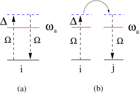
Figure 4: The off-resonant Raman scattering processes lead to the on-site term and the off-site term in Eqn.31.

The interaction between the two laser beams in Fig.1 with the two level bosonic atoms is:

$$H_{int} = \int d^{2}\vec{r}\Psi^{\dagger}(\vec{r})[\frac{\vec{p}^{2}}{2m_{a}}+V_{OL}(\vec{r})+\frac{\hbar\omega_{a}}{2}\sigma_{z}$$ (30)

$$+ \frac{\Omega}{2}\sum_{l}(e^{-i\omega_{l}t}\sigma^{+}u_{l}(\vec{r})+h.c.)]\Psi(\vec{r})$$

where $\Psi(\vec{r})=(\psi_{e},\psi_{g})$ is the two component boson annihilation operator, the incident and scattered lights in Fig.1a and the two incident lights in Fig.1b have frequencies $\omega_{l}$ and mode functions $u_{l}(\vec{r})=e^{i\vec{k}_{l}\cdot\vec{r}+i\phi_{l}}$ . The Rabi frequencies $\Omega$ are much weaker than the laser beams ( not shown in Fig.1 ) which form the optical lattices. In the following, we develop the formalism by using the light scattering geometry in Fig.1a which also applies to the atom scattering geometry in Fig.1b after some slight modifications. When it is far off the resonance, the laser light-atom detunings $\Delta_{l}=\omega_{l}-\omega_{a}$ where $\omega_{a}$ is the two level energy difference are much larger than the Rabi frequency $\Omega$ and the energy transfer $\omega=\omega_{1}-\omega_{2}$ ( See Fig.4 ), so $\Delta_{1}\sim\Delta_{2}=\Delta$. After adiabatically eliminating the upper level $e$ of the two level atoms, expanding the ground state atom field operator $\psi_{g}(\vec{r})=\sum_{i}b_{i}w(\vec{r}-\vec{r}_{i})$ in Eqn.30 where $w(\vec{r}-\vec{r}_{i})$ is the localized Wannier functions of the lowest Bloch band corresponding to $V_{OL}(\vec{r})$ and $b_{i}$ is the annihilation operator of an atom at the site $i$ in the Eqn.1, then we get the effective interaction between the off-resonant laser beams and the ground level $g$:

$$H_{int}=\hbar\frac{\Omega^{2}}{\Delta}e^{-i\omega t}[\sum^{N}_{i}J_{i,i}n_{i}+\sum^{N}_{<ij>}J_{i,j}b^{\dagger}_{i}b_{j}]$$ (31)

where the interacting matrix element is $J_{i,j}=\int d\vec{r}w(\vec{r}-\vec{r}_{i})u^{*}_{1}(\vec{r})u_{2}(\vec{r})w(\vec{r}-\vec{r}_{j})=J_{j,i}$. The first term in Eqn.31 is the on-site term $\hat{D}=\sum^{N}_{i}J_{i,i}n_{i}$ ( See Fig.4a ). The second term is the off-site term ( See Fig.4b ). Because the Wannier wavefunction $w(\vec{r})$ can be taken as real in the lowest Bloch band justify , the off-site term can be written as $\hat{K}=\sum^{N}_{<ij>}J_{i,j}b^{\dagger}_{i}b_{j}=\sum^{N}_{<ij>}J_{i,j}(b^{\dagger}_{i}b_{j}+h.c.)$ which is nothing but the off-site coupling to the nearest neighbor kinetic energy of the bosons $K_{ij}=b^{\dagger}_{i}b_{j}+h.c.$.

It is easy to show that:

$$\hat{D}(\vec{q})=f_{0}(\vec{q})\sum^{N}_{i=1}e^{-i\vec{q}\cdot\vec{r}_{i}}n_{i}=Nf_{0}(\vec{q})n(\vec{q})$$ (32)

where $\vec{q}=\vec{k}_{1}-\vec{k}_{0}$, $f_{0}(\vec{q})=\int d\vec{r}e^{-i\vec{q}\cdot\vec{r}}w^{2}(\vec{r})$ and $n(\vec{q})=\frac{1}{N}\sum^{N}_{i=1}e^{-i\vec{q}\cdot\vec{r}_{i}}n_{i}=\sum_{\vec{k}}b^{\dagger}_{\vec{k}}b_{\vec{k}+\vec{q}}$ is the Fourier transform of the density operator at the momentum $\vec{q}$. The wavevector is confined to $L^{-1}<q<a^{-1}$ where the trap size $L\sim 100\mu m$ and the lattice constant $a\sim 0.5\mu m$ in Fig.1. In fact, more information is encoded in the off-site kinetic coupling in Eqn.31. In a square lattice, the bonds are either oriented along the $\hat{x}$ axis $\vec{r}_{j}-\vec{r}_{i}=\hat{x}$ or along the $\hat{y}$ axis $\vec{r}_{j}-\vec{r}_{i}=\hat{y}$, we have:

$$\hat{K}_{\Box}=N[f_{x}(\vec{q})K_{x}(\vec{q})+f_{y}(\vec{q})K_{y}(\vec{q})]$$ (33)

where $K_{\alpha}(\vec{q})=\frac{1}{N}\sum^{N}_{i=1}e^{-i\vec{q}\cdot\vec{r}_{i}}K_{i,i+\alpha}=e^{iq_{\alpha}/2}\sum_{\vec{k}}\cos k_{\alpha}b^{\dagger}_{\vec{k}}b_{\vec{k}+\vec{q}}$ are the Fourier transform of the kinetic energy operator $K_{ij}=b^{\dagger}_{i}b_{j}+h.c.$ along $\alpha=x,y$ bonds at the momentum $\vec{q}$ and the ”form” factors $f_{\alpha}(\vec{q})=f(\vec{q},\vec{r}_{i}-\vec{r}_{j}=\alpha)=\int d\vec{r}e^{-i\vec{q}\cdot\vec{r}}w(\vec{r})w(\vec{r}+\vec{r}_{i}-\vec{r}_{j})$. Following the harmonic approximation used in boson , we can estimate that:

$$f_{0}(\pi,0) \sim e^{-\frac{1}{4}(V_{0}/E_{r})^{-1/2}}$$

$$f_{x}(\pi,0) \sim ie^{-\frac{1}{4}(V_{0}/E_{r})^{-1/2}-\frac{\pi^{2}}{4}(V_{0}/E_{r})^{1/2}}$$ (34)

so $|f_{x}(\pi,0)/f_{0}(\pi,0)|\sim e^{-\frac{\pi^{2}}{4}\sqrt{V_{0}/E_{r}}}$ where $V_{0}$ and $E_{r}=\hbar^{2}k^{2}/2m$ are the strength of the optical lattice potential and the recoil energy respectively boson . The $f_{0}(\pi,0)$ is close to 1 when $V_{0}/E_{r}>4$. It is instructive to relate this ratio to that of the hopping $t$ over the onsite interaction $U$ in the Eqn.1: $|f_{x}(\pi,0)/f_{0}(\pi,0)|\sim\frac{t}{U}\frac{a_{s}}{a}$ where $a_{s}$ is the zero field scattering length and $a=\lambda/2=\pi/k$ is the lattice constant, using the typical values $t/U\sim 10^{-1},a_{s}/a\sim 10^{-2}$, one can estimate $|f_{\alpha}/f_{0}|\sim 10^{-3}$. Note that the harmonic approximation works well only in a very deep optical lattice $V_{0}\gg E_{r}$, so the above value underestimates the ratio, so we expect $|f_{\alpha}/f_{0}|\geq 10^{-3}$.

The differential scattering cross section of the light from the cold atom systems in the Fig.1 can be calculated by using the standard linear response theory:

$$\frac{d\sigma}{d\Omega d\omega} = (\frac{\Omega^{2}}{\Delta})^{2}N^{2}[|f_{0}(\vec{q})|^{2}S_{n}(\vec{q},\omega)$$ (35)

$$+ \sum_{\alpha=\hat{x},\hat{y}}|f_{\alpha}(\vec{q})|^{2}S_{K_{\alpha}}(\vec{q},\omega)]$$

where $\vec{q}=\vec{k}_{1}-\vec{k}_{0},\omega=\omega_{1}-\omega_{2}$, the $S_{n}(\vec{q},\omega)=\langle n(-\vec{q},-\omega)n(\vec{q},\omega)\rangle$ is the dynamic density-density response function listed in Eqn.3 whose Lehmann representation was listed in braggbog . The $S_{K_{\alpha}}(\vec{q},\omega)=\langle K_{\alpha}(-\vec{q},-\omega)K_{\alpha}(\vec{q},\omega)\rangle$ is the bond-bond response function whose Lehmann representation can be got from that of the $S_{n}(\vec{q},\omega)$ simply by replacing the density operator $n(\vec{q})$ by the bond operator $K_{\alpha}(\vec{q})$.

The elastic scattering cross section $\frac{d\sigma}{d\Omega}|_{el}$ is proportional to:

$$\frac{d\sigma}{d\Omega}|_{el} = (\frac{\Omega^{2}}{\Delta})^{2}N^{2}[|f_{0}(\vec{q})|^{2}S_{n}(\vec{q},\omega=0)$$ (36)

$$+ \sum_{\alpha=\hat{x},\hat{y}}|f_{\alpha}(\vec{q})|^{2}S_{K_{\alpha}}(\vec{q},\omega=0)]$$

The integrated differential scattering cross section over the final energy $\frac{d\sigma}{d\Omega}=\int d\omega\frac{d\sigma}{d\Omega d\omega}$ is proportional to the equal-time response function is

$$\frac{d\sigma}{d\Omega} = (\frac{\Omega^{2}}{\Delta})^{2}N^{2}[|f_{0}(\vec{q})|^{2}S_{n}(\vec{q})$$ (37)

$$+ \sum_{\alpha=\hat{x},\hat{y}}|f_{\alpha}(\vec{q})|^{2}S_{K_{\alpha}}(\vec{q})]$$

In the following, we will discuss the physical implications of Eqn.35 on the CDW, VBS and corresponding supersolids summarized in the Sec.II.

IV Superfluid, Mott insulator and Superfluid to Mott transition at integer fillings

Quantum phase transitions are characterized by three critical exponents $z,\nu,\eta$ called ” two scale factor” universality. It is well known that the SF to Mott transition is described by the relativistic effective action bipart :

$${\cal S}=\int d^{2}rd\tau[|\partial_{\tau}\phi|^{2}+|\nabla\phi|^{2}+r|\phi|^{2}+u|\phi|^{4}+\cdots]$$ (38)

where in the Mott state $r>0,\langle\phi\rangle=0$, while in the SF phase $r<0,\langle\phi\rangle\neq 0$. The SF to Mott transition described by Eqn.38 is in the $3d$ XY universality class with the critical exponents $z=1,\nu=0.67,\eta=0.04$ ( Note that for $d=1$, it is in $2d$ XY universality class, namely, KT transition ). In the following, we will discuss the elastics and the in-elastic scattering at the SF and Mott, then the quantum phase transition between the two phases respectively. As shown in the Sect.III, the scattering cross sections are determined by the density-density correlation functions, so we will focus on their computations. Although the order parameter correlation functions were well studied theoretically from both the direct and dual pictures, they can not be directly measured by experiments yet. The density-density correlation functions have not been discussed theoretically so far.

IV.1 Elastics scattering at the reciprocal lattice vector $\vec{K}$ to detect SF and Mott states

We first look at the superfluid to Mott transition at integer filling factor $n$. When $\vec{q}$ is equal to the shortest reciprocal lattice vector $\vec{K}=(2\pi,0)$, in the Mott state, $\frac{d\sigma^{M}}{d\Omega}=|f^{M}_{0}(2\pi,0)|^{2}N^{2}n^{2}$, in the superfluid state, $\frac{d\sigma^{SF}}{d\Omega}=|f^{SF}_{0}(2\pi,0)|^{2}N^{2}n^{2}+2|f^{SF}_{x}(2\pi,0)|^{2}N^{2}B^{2}$ where $B$ is the average kinetic energy on a bond in the superfluid side. Because $|f^{SF}_{0}(2\pi,0)|^{2}\sim|f^{M}_{0}(2\pi,0)|^{2}\sim 1$ and $B$ is appreciable only in the superfluid side, we expect an increase of the scattering cross section:

$$\frac{d\sigma^{SF}}{d\Omega}-\frac{d\sigma^{M}}{d\Omega}\sim 2|f^{SF}_{x}(2\pi,0)|^{2}N^{2}B^{2}$$ (39)

across the Mott to the SF transition due to the prefactor $N^{2}$. The increase is most evident when moving from well inside the Mott phase to well inside the SF phase. This increase may be used as an effective measure of the boson kinetic energy inside the SF. This prediction could be tested immediately. Surprisingly, there is no such optical Bragg scattering experiment in the superfluid yet.

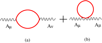
Figure 5: The current-current correlator. Its $\mu=\nu=0$ component leads to the boson density-density correlation function Eqn.42. Although the $D=3+1$ case was well documented ryder . The $D=2+1$ case seems not be calculated yet and was done in the Sec.IV-b.

IV.2 In-elastics scattering slightly away from a reciprocal lattice vector $\vec{K}$ to detect the excitation spectrum in SF and Mott states

Now we study the in-elastic scattering away from zero ( or any other reciprocal lattice vector $\vec{K}$. ). The excitation spectrum inside a SF was already given in Eqn.8 and Eqn.10. Here, from the effective theory of both boson and dual vortex pictures, we will calculate the density-density correlation function not only in the SF side, but also in the Mott side and the quantum critical point.

(1) Density-density correlation functions from a direct boson picture

Observing that the density $n=\phi^{\dagger}\partial_{\tau}\phi-(\partial_{\tau}\phi^{\dagger})\phi$ is a conserved quantity. In order to calculate the density-density correlation function, we add a source term to Eqn.38

$${\cal S}[A_{\mu},\phi]=\int d^{2}rd\tau[|(\partial_{\mu}-iA_{\mu})\phi|^{2}+m^{2}|\phi|^{2}+u|\phi|^{4}+\cdots]$$ (40)

In the Mott side, $m^{2}>0$, Then integrating out the massive $\phi$ field according to the Feymann diagram Fig.5 paying special attentions to the diamagnetic term in Fig.5b, one gets

$${\cal S}[A_{\mu}] = \frac{1}{2}A_{\mu}(-k)\Pi_{\mu\nu}(k)A_{\nu}(k)+\cdots$$

$$\Pi_{\mu\nu}(k) = \frac{m}{2\pi}[\frac{k_{\mu}k_{\nu}}{k^{2}}-\delta_{\mu\nu}](I(z)-1),~{}~{}z=\frac{k^{2}}{m^{2}}$$ (41)

where $I(z)=\int^{1}_{0}dx[1+x(1-x)z]^{1/2}=\frac{1}{2}+\frac{(4+z)}{4\sqrt{z}}\arctan\frac{\sqrt{z}}{2}=1+\frac{z}{12}-\frac{z^{2}}{240}+\cdots$ as $z\rightarrow 0$.

Using $A_{\mu}=(A_{0},A_{\alpha})$ and $k=(\omega,\vec{q})$ and putting $\mu=\nu=0$, we can get the boson density-density correlation function:

$$S^{Mott}_{n}(\vec{q},\omega)=\Pi_{00}(\vec{q},\omega)=\frac{5m}{6\pi}\frac{q^{2}}{\omega^{2}+q^{2}+20m^{2}}$$ (42)

where one can identify the Mott gap $\Delta^{2}_{Mott}=20m^{2}$. The compressibility

$$\kappa_{Mott}=S(\vec{q}\rightarrow 0,\omega=0)\sim q^{2}\rightarrow 0$$ (43)

which, namely, in-compressible inside the Mott state as expected. Again,

One can evaluate immediately the structure factor

$$S^{Mott}_{n}(\vec{q})=\frac{5m}{12\pi}\frac{q^{2}}{\sqrt{q^{2}+20m^{2}}}$$ (44)

At the quantum critical point between the SF and the Mott phase, $m\rightarrow 0$, $z\rightarrow\infty$, then $I(z)\rightarrow\sqrt{z}\int^{1}_{0}\sqrt{x(1-x)}=\frac{\pi}{8}\sqrt{z}$, we get

$$S^{QC}_{n}(\vec{q},\omega)=\frac{1}{16}\frac{q^{2}}{\sqrt{\omega^{2}+q^{2}}}$$ (45)

which shows that

$$\kappa_{QC}=S(\vec{q}\rightarrow 0,\omega=0)\sim q\rightarrow 0$$ (46)

which, namely, still in-compressible at the QC point.

One can evaluate immediately the dynamic structure factor

$$S^{QC}_{n}(\vec{q})\sim q^{2}\log\Lambda/q$$ (47)

where the $\Lambda\sim 1/a$ is the ultra-violet frequency cutoff.

Inside the superfluid $m^{2}<0$, then it is convenient to write $V(\phi)=\frac{1}{4}\lambda(|\phi|^{2}-a^{2})^{2}$. We write the order parameter in the polar coordinate $\phi=\sqrt{a^{2}+\delta\rho}e^{i\phi}$, then Eqn.38 becomes:

$${\cal L} = (a^{2}+\delta\rho)(\partial_{\mu}\theta)^{2}+\cdots$$ (48)

$$+ \frac{1}{4}(a^{2}+\delta\rho)^{-1}(\partial_{\mu}\delta\rho)^{2}+\frac{1}{4}\lambda(\delta\rho)^{2}$$

where one can see that there is a gapless ( Goldstone ) $\theta$ mode and the massive Higgs magnitude $\delta\rho$ fluctuation mode. It is important to stress that the density operator is different than the Higgs magnitude fluctuation operator. The former is a conserved quantity, while the later is not, although both are $U(1)$ invariant. So they have different correlation functions. Unfortunately, it is not straightforward to extract the density-density correlation function Eqn.8 inside a SF from Eqn.48. However, as shown below, it can be easily derived from the dual vortex picture.

In a brief summary, Eqn.8, 42, 45 describes the density-density correlation functions in the SF, Mott and the QC regimes respectively. In the Mott state, when $q\ll m$, one can see $S^{Mott}(\vec{q})\sim q^{2}$ which is in sharp contrast to that inside a superfluid $S^{SF}(\vec{q})\sim q$. While at the QC, $S^{QC}(\vec{q})\sim q^{2}\log\Lambda/q$. Note that all the compressibilities at Mott, SF and QC can also be directly measured by the in situ method at different positions inside a trap insitu0 ; insitu1 .

The scattering cross section at the classical diffraction minimum $\vec{q}=(\pi,\pi)$ will be computed in the Appendix B.

(2) The density-density correlation functions from a dual vortex picture

Alternatively, one can calculate the density-density correlation from the dual vortex action bipart ; hightc . It is well known that the boson action Eqn.38 is dual to the vortex action:

$${\cal S}_{d}[a_{\mu},\psi] = \int d^{3}x[|(\partial_{\mu}-ia_{\mu})\psi_{v}|^{2}+r_{d}|\psi_{v}|^{2}+u_{d}|\psi_{v}|^{4}+\cdots$$ (49)

$$+ \frac{1}{4e^{2}}f^{2}_{\mu\nu}]$$

where in the Mott state $r_{d}<0,\langle\psi_{v}\rangle\neq 0$, while in the SF phase $r_{d}>0,\langle\psi_{v}\rangle=0$ with also the $3d$ XY critical exponents $z=1,\nu=0.67,\eta=0.04$.

In the Mott state, the vortex condensation $\langle\psi_{v}\rangle\neq 0$ leads to a mass term for the gauge field $\frac{1}{2}|\langle\psi_{v}\rangle|^{2}(a^{t}_{\mu})^{2}$ where $a^{t}_{\mu}$ is the transverse component of the gauge field. In the Landau gauge $\partial_{\mu}a_{\mu}=0$, the effective action for the gauge field is:

$${\cal S}_{d}[a_{\mu}] = \frac{1}{2}a_{\mu}(-k)[\frac{k^{2}}{e^{2}}(\delta_{\mu\nu}-\frac{k_{\mu}k_{\nu}}{k^{2}})+\frac{1}{\alpha}k_{\mu}k_{\nu}$$ (50)

$$+ |\langle\psi\rangle|^{2}(\delta_{\mu\nu}-\frac{k_{\mu}k_{\nu}}{k^{2}})]a_{\nu}(k)$$

where $\alpha\rightarrow 0$ indicates the Landau gauge.

Using $a_{\mu}=(a_{0},\vec{a})$ and $k=(\omega,\vec{q})$, we can find the density-density correlation inside the Mott phase:

$$S^{Mott}_{n}(\vec{q},\omega)=\langle(\nabla\times\vec{a})(\nabla\times\vec{a})\rangle=\frac{e^{2}q^{2}}{\omega^{2}+q^{2}+m^{2}_{d}}$$ (51)

where $m^{2}_{d}=e^{2}|\langle\psi_{v}\rangle|^{2}$. We can identify the quasi-particle spectral weight ${\cal A}=e^{2}$. It is identical to Eqn.42 after we identify $m^{2}_{d}=20m^{2}$.

Inside the superfluid state $r_{d}>0$, the mass term for the gauge field is absent, integrating out the massive vortex fluctuation leads to the density-density correlation inside the superfluid phase:

$$S^{SF}_{n}(\vec{q},\omega)=\langle(\nabla\times\vec{a})(\nabla\times\vec{a})\rangle=\frac{e^{2}q^{2}}{\omega^{2}+q^{2}}$$ (52)

which is identical to Eqn.8 after putting back the corresponding the superfluid density $\rho_{s}$ and the phonon velocity $v^{2}$.

At the quantum critical point between the SF and the Mott phase, integrating out the massless vortex fluctuation leads to the density-density correlation at the QC:

$$S^{QC}_{n}(\vec{q},\omega)\sim\langle(\nabla\times\vec{a})(\nabla\times\vec{a})\rangle=\frac{q^{2}}{\sqrt{\omega^{2}+q^{2}}}$$ (53)

which is identical to Eqn.45 from the direct boson picture. Eqn.47 follows.

IV.3 The scaling functions for the density-density correlation functions across the SF to Mott transition

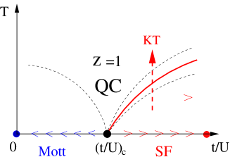
Figure 6: Finite temperature phase diagram of the SF to Mott transition. There are 3 fixed points: the Mott fixed point at $t/U=0$, the SF fixed point at $t/U=\infty$ and the quantum critical point at $(t/U)_{c}$. The QC is the quantum Critical regime. The KT stands for the Kosterlize-Thouless transition. See Fig.12 for the zero temperature phase diagram and the phases inside a trap.

So far, we discussed the properties of different quantum phases where mean field theory works well. It is important to study quantum fluctuations near the quantum critical point between different quantum phases. Ref.boson0 focused on the scaling form of the single particle Green function $\langle\phi^{\dagger}(\vec{x},\tau)\phi(0,0)\rangle$. Here, motivated by the light scattering experiments, we are studying the scaling form of the density-density correlation function $\langle\delta n(\vec{x},\tau)\delta n(0,0)\rangle$ where $\delta n=\phi^{\dagger}\partial_{\tau}\phi-(\partial_{\tau}\phi^{\dagger})\phi$. Following the scaling theory developed in scaling and observing $\delta n$ is a conserved quantity, we can write down the scaling functions near the SF to Mott transition in Fig.6:

$$S^{SF}_{n}(\vec{q},\omega,k_{B}T)=|C|^{2}\frac{k_{B}T}{v^{2}}\Phi_{SF}(\frac{\hbar vq}{k_{B}T},\frac{\hbar\omega}{k_{B}T},\frac{k_{B}T}{2\pi\rho_{s}})$$ (54)

In the Mott state $2\pi\rho_{s}$ should be replaced by the Mott gap $\Delta$. At the QC, $\Phi_{SF}(\frac{\hbar vq}{k_{B}T},\frac{\hbar\omega}{k_{B}T},\infty)=\Phi_{Mott}(\frac{\hbar vq}{k_{B}T},\frac{\hbar\omega}{k_{B}T},\infty)$. Note that due to $z=1$, the spin wave velocity $v$ remains not critical across the SF to Mott transition in Fig.6, while $\rho_{s}\sim(t-t_{c})^{(d+z-2)\nu}\sim(t-t_{c})^{\nu}$ with $z=1,d=2$ and $\Delta\sim(t_{c}-t)^{\nu},\nu\sim 0.67$.

Note that Eqn.8 in the SF and Eqn.42 in the Mott side only work deep inside the two phases controlled by the SF fixed point and the Mott fixed point in Fig.6 respectively, but will break down near to the QCP. The equal time correlation function follow from $\int\frac{d\omega}{2\pi}$ over Eqn.54.

At $T=0$, Eqn.54 simplifies to

$$S^{SF}_{n}(\vec{q},\omega,T=0)=|C|^{2}\frac{2\pi\rho_{s}}{v^{2}}\Phi_{SF}(\frac{\hbar vq}{2\pi\rho_{s}},\frac{\hbar\omega}{2\pi\rho_{s}})$$ (55)

In the Mott state $2\pi\rho_{s}$ should be replaced by the Mott gap $\Delta$. From Eqn.8, we can determine that $\Phi_{SF}(x,y)=\frac{x^{2}}{x^{2}+y^{2}}$. From Eqn.42, we can determine that $\Phi_{Mott}(x,y)=\frac{x^{2}}{x^{2}+y^{2}+1}$.

At the QC $\rho_{s}=\Delta=0$, Eqn.55 simplifies further to

$$S^{QC}_{n}(\vec{q},\omega,T=0)=|C|^{2}\frac{\hbar vq}{v^{2}}\Phi_{QC}(\frac{\hbar\omega}{\hbar vq})$$ (56)

From Eqn.45, we can determine that $\Phi_{QC}(x)=\frac{1}{\sqrt{x^{2}+1}}$.

V CDW and CDW supersolid at and near half fillings

Figure 7: The characteristics of optical scattering cross section in a square lattice.(a) CDW, the ratio of the peak at $\vec{Q}_{n}$ over that at $\vec{K}$ is $\sim m^{2}/n^{2}\sim 1$. (b) VBS state, the ratio of the peak at $\vec{Q}_{K}$ over that at $\vec{K}$ is $\sim|f_{x}/f_{0}|^{2}K^{2}/n^{2}\sim 10^{-5}$. It should be visible in the current optical Bragg scattering experiments.

At the $1/2$ filling along the horizontal axis in Fig.3a, inside the SF state near the CDW, there is a peak of $S_{n}(\vec{q})$ near $\vec{Q}_{n}=(\pi,\pi)$, so the SF to the CDW transition is a first order one driven by the instability of the peak. Due to the lack of VBS order on both sides, the second term in Eqn.35 can be neglected, so that

$$\frac{d\sigma}{d\Omega dE}|_{CDW}\sim(\frac{\Omega^{2}}{\Delta})^{2}N^{2}|f_{0}(\vec{q})|^{2}S_{N}(\vec{q},\omega)$$ (57)

(a) Elastic scattering at the CDW and CDW-SS ordering vector $\vec{Q}_{n}$.

When one gets into the CDW state at $\vec{Q}_{n}$ in Fig.3b in bipart , then the $S_{n}(\vec{q})$ should show a peak at $\vec{q}=\vec{Q}_{n}$ whose amplitude scales as the square of the number of atoms inside the trap $S_{CDW}(\vec{Q}_{n})\sim|f_{0}(\pi,\pi)|^{2}N^{2}m^{2}$ where $m=n_{A}-n_{B}$ is the CDW order parameter bipart . When $\vec{q}=\vec{K}$, then $S_{CDW}(\vec{K})\sim|f_{0}(2\pi,0)|^{2}N^{2}n^{2}$ where $f_{0}(2\pi,0)\sim f^{2}_{0}(\pi,\pi)$ ( Fig.7a ). So the ratio of the two peaks in Fig.7a is $S_{CDW}(\vec{Q}_{n})/S_{CDW}(\vec{K})\sim m^{2}/n^{2}$ if one neglects the small difference of the two form factors. Slightly away from $1/2$ filling, the CDW in Fig.3a may turn into the CDW supersolid ( CDW-SS ) phase through a second order phase transition described by Eqn.58. Then we have $\langle n(\vec{q})\rangle=m\delta_{\vec{q},\vec{Q}_{n}}+n\delta_{\vec{q},0}$ where $n=n_{A}+n_{B}=1/2+\delta n$. The superfluid density $\rho_{s}\sim\delta n=n-1/2$. The scattering cross section inside the CDW-SS at $\vec{Q}_{n}$ : $S_{CDW-SS}(\vec{Q}_{n})\sim|f_{0}(\pi,\pi)|^{2}N^{2}m^{2}$ stays more or less the same as that inside the CDW, but at $\vec{K}=(2\pi,0)$: $S_{CDW-SS}(\vec{K})\sim|f_{0}(2\pi,0)|^{2}N^{2}n^{2}+2|f_{x}(2\pi,0)|^{2}N^{2}(\delta n)^{2}B^{2}$ will increase where $n=1/2+\delta n$. The $B$ is the average bond strength due to very small superfluid component $\rho_{s}\sim\delta n=n-1/2$ flowing through the whole lattice. So we expect the right peak in Fig.7a will increase due to the increase of the total density and the superfluid component inside the CDW-SS phase. Of course, the small superfluid component at $\vec{k}=0$ can also be detected by the TOF with the peak strength near $\vec{k}=0$ proportional to $\rho_{s}\sim\delta n$.

(b) In-elastics scattering to detect the excitation spectrum in CDW and CDW-SS

So far, we only discussed the ground state properties of various quantum states. The elementary excitation spectrum above these ground states can be determined from the peak positions of the corresponding dynamic density-density or bond-bond response functions. Eqn.35 shows that the response function of the cold atom system is the sum of the two response functions with the corresponding spectral weight $\sim|f_{0}|^{2}$ and $\sim|f_{\alpha}|^{2}$. The $\langle\delta n\delta n\rangle$ correlation function inside a SF was studied in several different physical systems in ssorder ; sforder and was listed in Eqn.8 and 10. In the SF near to the CDW, there is a roton minimum near $\vec{q}=\vec{Q}_{n}$, the $S_{n}(\vec{q})$ shows a peak near $\vec{Q}_{n}$ in Fig.8a1. The superfluid mode in the Fig.8a1 has a spectral weight $\sim N|f_{0}|^{2}\times\rho_{s}$ where $\rho_{s}\sim n$. Inside the CDW-SS, the roton minimum disappears and is replaced by the upper branch with a CDW gap $\Delta_{CDW}\sim U$ and a spectral weight $\sim N|f_{0}|^{2}\times 1/2$ in the Fig.8b1, the lower superfluid branch in the Fig.8b1 has a spectral weight $\sim N|f_{0}|^{2}\times\rho_{s}$ where $\rho_{s}\sim\delta n=n-1/2$ is the superfluid density inside the CDW-SS. Inside the CDW, the superfluid lower branch disappears, the upper CDW branch in Fig.8c1 has the spectral weight $\sim N|f_{0}|^{2}\times 1/2$.

Figure 8: The excitations spectrum in the CDW, VBS, SF, CDW-SS and VB-SS states which are the peak positions of the corresponding dynamic response functions shown with arrows. In the (b1) and (c1) cases, the starting wavevector is $\vec{Q}_{n}$ in the upper CDW branch. In the (b2) and (c2) cases, the starting wavevector is $\vec{Q}_{K}$ in the upper VBS branch. The corresponding spectral weights are worked out in the text.

(c) Scaling function across the CDW to CDW-SS transition.

Slightly away from $1/2$ filling, the transition from the CDW to the CDW-SS along the vertical axis in Fig.3b is described by the non-relativistic effective action bipart :

$${\cal S}_{non}=\int d^{2}rd\tau[\phi^{\dagger}\partial_{\tau}\phi+\frac{\hbar^{2}}{2m_{a}}|\nabla\phi|^{2}-\mu|\phi|^{2}+u|\phi|^{4}+\cdots]$$ (58)

with the critical exponents $z=2,\nu=1/2,\eta=0$ with logarithmic corrections bipart .

It is the chemical potential $\mu$ tuning the zero density transition from the CDW at $\mu<0$ with $\langle\phi\rangle=0$ to the CDW-SS with $\mu>0$ with $\langle\phi\rangle\neq 0$, so the critical chemical potential $\mu_{c}=0$. Well inside the CDW-SS phase, one can set $\langle\phi\rangle=|\langle\phi\rangle|e^{i\theta}$, then the linear derivative term in Eqn.58 becomes irrelevant, the density-density correlation function of the SF component reduces to Eqn.8 with $\rho_{s}\sim\frac{\hbar^{2}|\langle\phi\rangle|^{2}}{2m}$. It leads to the lower branch in Fig.8b1.

Ref.z2 focused on the scaling form of the single particle Green function $\langle\phi^{\dagger}(\vec{x},\tau)\phi(0,0)\rangle$. Here, motivated by the light scattering experiments, we are studying the scaling form of the density-density correlation function $\langle\delta n(\vec{x},\tau)\delta n(0,0)\rangle$ where $\delta n/a^{2}=\phi^{\dagger}\phi$ is the density above the CDW background. Near the QCP, we have $\langle n(\vec{q})\rangle=m\delta_{\vec{q},\vec{Q}_{n}}+n\delta_{\vec{q},0}$ where $n=n_{A}+n_{B}=1/2+\delta n$. Because $\delta n/a^{2}=\phi^{\dagger}\phi$ is a conserved quantity, so it has no anomalous dimension. From the scaling analysis in z2 , one can show that at $T=0$

$$\delta n=\frac{m_{a}\mu a^{2}}{4\pi\hbar^{2}}\ln[\frac{\hbar^{2}}{2m_{a}\mu a^{2}}]$$ (59)

where $a$ is the lattice constant and $m_{a}$ is the effective atom mass in Eqn.58 and 30, the logarithmic factor is also explicitly written.

The superfluid density inside the CDW-SS is $\rho_{s}\sim(\mu-\mu_{c})^{(d+z-2)\nu}\sim\mu-\mu_{c}$ with $d=2,z=2,\mu=1/2,\eta=0$ upto a logarithmic correction. From Eqn.59, we expect that

$$\rho_{s}\sim\frac{m_{a}\mu a^{2}}{4\pi\hbar^{2}}\ln[\frac{\hbar^{2}}{2m_{a}\mu a^{2}}]$$ (60)

where we set $\mu_{c}=0$.

In the scaling limit $q\ll 1/a,\hbar\omega\ll\frac{\hbar^{2}}{2m_{a}a^{2}}$, the density-density correlation function should take the following scaling form:

$$S_{n}(\vec{q},\omega)=\frac{2m_{a}a^{4}}{\hbar}\Phi_{n}(\frac{\hbar\omega}{k_{B}T},\frac{\hbar q}{\sqrt{2m_{a}k_{B}T}},\frac{\mu}{k_{B}T})$$ (61)

where $\Phi_{n}$ is a universal function independent of the atom-atom interactions in Eqn.1. Inside the CDW-SS phase in Fig.3b, there should also be a $S_{n}(\vec{q})$ peak $\sim|f_{0}|^{2}N^{2}m^{2}$ at $\vec{q}=\vec{Q}_{n}$ signaling its CDW order.

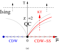
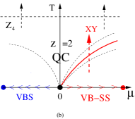
Figure 9: (a) The CDW to CDW-SS driven by the chemical potential $\mu$. The dashed line is a finite temperature Ising melting transition. (b) The VBS to VB-SS driven by the chemical potential $\mu$. The dashed line is a finite temperature $Z_{4}$ Clock melting transition. See also Fig.3 for the zero temperature phase diagram and Fig.13 for the phases inside a trap.

In fact, Eqns.59,60, 61 should also apply to the the Mott to SF transition and the CDW to the CDW-SS inside an harmonic trap driven by a local chemical potential ( or equivalently the distance from the center to the boundary ) under the LDA and will be discussed in Sec. XI.

VI VBS and VB supersolid at and near half fillings

At the $1/2$ filling along the horizontal axis in Fig.3b, inside the SF state near the VBS, there is a peak of $S_{K}(\vec{q})$ near $\vec{Q}_{K}=(\pi,0)$, so the SF to the VBS transition is a very weak first order one.

(a) Elastic scattering at the VBS and VB-SS ground state at its ordering wavevector $\vec{Q}_{K}$.

When $\vec{q}=\vec{K}$, due to the uniform distribution of the density in the VBS, the second term in Eqn.35 can be neglected, so there is a diffraction peak ( Fig.7b ) whose amplitude scales as the square of the number of atoms inside the trap $S_{VBS}(\vec{K})\sim|f_{0}(2\pi,0)|^{2}N^{2}n^{2}$ where $f_{0}(2\pi,0)\sim f^{4}_{0}(\pi,0)$ and $n=1/2$ is the uniform density in the VBS state.

However, when one tunes $\vec{q}$ near $\vec{Q}_{K}$, the first term in Eqn.35 can be neglected, then

$$\frac{d\sigma}{d\Omega dE}|_{VBS}\sim(\frac{\Omega^{2}}{\Delta})^{2}N^{2}\sum_{\alpha=\hat{x},\hat{y}}|f_{\alpha}(\vec{q})|^{2}S_{K_{\alpha}}(\vec{q},\omega)$$ (62)

It should show a peak at $\vec{q}=\vec{Q}_{K}$ signifying the VBS ordering at $\vec{Q}_{K}$ whose amplitude scales also as the square of the number of atoms inside the trap $S_{VBS}(\vec{Q}_{K})\sim|f_{x}(\pi,0)|^{2}N^{2}K^{2}$ where $K=K_{x}-K_{y}$ is the VBS order parameter bipart . So the ratio of the VBS peak at $\vec{q}=\vec{Q}_{K}$ over the uniform density peak at $\vec{q}=\vec{K}$ is $S_{VBS}(\vec{Q}_{K})/S_{VBS}(\vec{K})\sim|f_{x}(\pi,0)/f_{0}(2\pi,0)|^{2}\geq 10^{-5}$. However, the smallness of $|f_{x}|^{2}$ is compensated by the large number of atoms $N\sim 10^{6}$, $|f_{x}|^{2}N^{2}=(|f_{x}|^{2}N)\times N\sim N\sim 10^{6}$. Therefore, the Bragg scattering cross section from the VBS order is $\geq 10^{-5}$ smaller than that at $\vec{q}=\vec{K}$ at the same incident energy $I_{in}$ ( Fig.7b ), but still $\sim 10^{6}$ above the background, so very much visible in the current optical Bragg scattering experiments. Slightly away from $1/2$ filling, the VBS may turn into VB Supersolid (VB-SS) through a second order transition bipart . We have $\langle K_{x}(\vec{q})\rangle=B\delta_{\vec{q},0}+K\delta_{\vec{q},\vec{Q}_{K}}$ and $\langle n(\vec{q})\rangle=(\delta n+1/2)\delta_{\vec{q},0}$. The superfluid density $\rho_{s}\sim\delta n=n-1/2$. The scattering cross section inside VB-SS: $S_{VB-SS}(\vec{Q}_{K})\sim|f_{x}(\pi,0)|^{2}N^{2}K^{2}$ stays more or less the same as that inside the VBS, but $S_{VB-SS}(\vec{K})\sim|f_{0}(2\pi,0)|^{2}N^{2}n^{2}+|f_{x}(2\pi,0)|^{2}N^{2}(\delta n)^{2}B^{2}_{x}+|f_{y}(2\pi,0)|^{2}N^{2}(\delta n)^{2}B^{2}_{y}$ where $n=1/2+\delta n$ and the $B_{x},B_{y}$ are the average bond strengths along $x$ and $y$ due to very small superfluid component $\rho_{s}\sim\delta n=n-1/2$ flowing through the whole lattice. So we expect the right peak in Fig.7b will increase due to the increase of the total density and the superfluid component inside the VB-SS phase. Of course, the superfluid component at $\vec{k}=0$ can also be detected by the TOF with the peak strength near $\vec{k}=0$ proportional to $\rho_{s}\sim\delta n$. Very similarly, one can discuss the VBS order at $\vec{q}=\vec{Q}_{K}=(0,\pi)$. For the plaquette VBS order in Fig.2 which has both $(\pi,0$ and $(0,\pi)$ order, then one should be able to see the $S_{K}(\vec{q})$ peaks at both $(\pi,0)$ and $(0,\pi)$. So the dimer VBS and the plaquette VBS can also be distinguished by the optical Bragg scattering.

(b) In-elastics scattering to detect the excitation spectrum in VBS and VB-SS

In the SF near to the VB, there is no peak in $S_{n}(\vec{q})$. The superfluid mode in the Fig.8a2 has a spectral weight $\sim N|f_{0}|^{2}\times\rho_{s}$ where $\rho_{s}\sim n$. However, $S_{VBS}(\vec{q})$ shows a peak near $\vec{Q}_{K}$ which is suppressed by a factor $|f_{x}|^{2}$ as compared to Fig.8a1. Inside the VB-SS, the SF order of the VB-SS is the same as the SF inside the CDW-SS, so its $\langle\delta n\delta n\rangle$ correlation function is also given by Eqn.8. So there is a upper branch with a VBS gap $\Delta_{VBS}\sim t^{2}/U$ and a spectral weight $\sim N|f_{x}|^{2}\times 1/2$ in the Fig.8b2, also a lower superfluid branch in the Fig.8b2 with the spectral weight $\sim N|f_{0}|^{2}\times\rho_{s}$ where $\rho_{s}\sim\delta n=n-1/2$ is the superfluid density inside the VB-SS. Inside the VBS, the superfluid lower branch disappears, the upper VBS branch in Fig.8c2 has the spectral weight $\sim N|f_{x}|^{2}\times 1/2$.

(c) The transition from the VBS to the VB-SS

Slightly away from $1/2$ filling, the transition from the VBS to the VB-SS along the vertical axis in Fig.3b near $\vec{q}=(0,0)$ is also described by Eqn.58, so it is also in the same universality class of SF to Mott transition with the critical exponents $z=2,\nu=1/2,\eta=0$ upto a logarithmic correction bipart . Eqn.59 and Eqn.61 also hold with $\delta n=\phi^{\dagger}\phi$ as the boson density above the VBS background.

VII Detection of quantum phases in frustrated lattices

The procedures discussed in bipartite lattices in the previous sections can be generalized to frustrated lattices such as triangular and kagome lattices. There are several new features due to the frustrations (1) The ordering wavevector $\vec{Q}_{n}\neq-\vec{Q}_{n}$, while for a bi-partite lattice $\vec{Q}_{n}=-\vec{Q}_{n}$ upto a reciprocal lattice. (2) The corresponding fluctuation near the ordering wavevector $\vec{Q}_{n}$ will be a complex order parameter, in contrast to that on a bipartite lattice which is just a real ( or Ising ) order parameter. The results achieved should also be useful to Quantum Monte Carlo simulations on the extended boson Hubbard model in a frustrated finite $N=L\times L$ lattice frusqmc . The analysis in the direct picture in this section can be contrasted to that by the dual vortex method in the dual picturefrus . Several important CDW, VBS and CDW-VBS phases are reviewed in the appendix A.

VII.1 Density-Density and bond-bond correlation functions in a frustrated lattice

In a frustrated lattice, in general, one can write the density at site $i$ as

$$N(\vec{r}_{i},t)=n(\vec{r}_{i},t)+Re\sum^{P}_{\alpha=1}\phi_{\alpha}e^{i\vec{Q}_{\alpha}\cdot\vec{r}_{i}}$$ (63)

where $\vec{Q}_{\alpha},\alpha=1,2,\cdots,P$ are the ordering wavevectors, the $\phi_{\alpha}$ is the complex CDW order parameter near the $\vec{Q}_{\alpha}$. For the X-CDW in Fig.14a, $P=1$, for the CDW-VBS in Fig.15, $P=3$. Then the density-density correlation function in Eqn.3 can be written as:

$$S_{N}(\vec{q},t) = \frac{1}{N}\sum_{i}e^{-i\vec{q}\cdot\vec{r}_{i}}\langle n(i,t)n(0,0)\rangle_{C}+n^{2}\delta_{\vec{q},0}$$ (64)

$$+ \sum^{P}_{\alpha=1}[\frac{1}{N}\sum_{i}e^{-i(\vec{q}-\vec{Q}_{\alpha})\cdot\vec{r}_{i}}\langle\phi_{\alpha}(i,t)\phi^{*}_{\alpha}(0,0)\rangle_{C}$$

$$+ \frac{1}{N}\sum_{i}e^{-i(\vec{q}+\vec{Q}_{\alpha})\cdot\vec{r}_{i}}\langle\phi^{*}_{\alpha}(i,t)\phi_{\alpha}(0,0)\rangle_{C}]$$

$$+ \sum^{P}_{\alpha=1}|\langle\phi_{\alpha}\rangle|^{2}(\delta_{\vec{q},\vec{Q}_{\alpha}}+\delta_{\vec{q},-\vec{Q}_{\alpha}})$$

where we have used the translational invariance to get rid of one summation and $\langle n_{i}(t)n_{j}(0)\rangle_{C}=\langle n_{i}(t)n_{j}(0)\rangle-n^{2}$ and $\langle\phi^{*}_{\alpha}(i,t)\phi_{\alpha}(0,0)\rangle_{C}=\langle\phi^{*}_{\alpha}(i,t)\phi_{\alpha}(0,0)\rangle-|\langle\phi_{\alpha}\rangle|^{2}$ are connected Green functions. The $\langle\phi_{\alpha}\rangle=m_{\alpha}e^{i\theta_{\alpha}}$ is the expectation value of the CDW order parameter. The translational invariance also dictates $\langle\phi^{*}_{\alpha}(i,t)\phi_{\beta}(0,0)\rangle=0$ for $\alpha\neq\beta$.

Its Fourier transform leads to the dynamic structure function:

$$S_{N}(\vec{q},\omega) = \int dte^{-i\omega t}S_{N}(\vec{q},t)$$ (65)

$$= n^{2}\delta_{\vec{q},0}\delta(\omega)+\sum^{P}_{\alpha=1}|\langle\phi_{\alpha}\rangle|^{2}(\delta_{\vec{q},\vec{Q}_{\alpha}}+\delta_{\vec{q},-\vec{Q}_{\alpha}})\delta(\omega)$$

$$+ \frac{1}{N}S^{inel}_{n}(\vec{q},\omega)+\frac{1}{N}S^{inel}_{\phi}(\vec{q},\omega)$$

where the first and second $\delta(\omega)$ terms denote the elastic scatterings at $\vec{q}=0$ and $\vec{q}=\vec{Q}_{\alpha}$ respectively, the third and the fourth term denote the inelastic scatterings near $\vec{q}=0$ and $\vec{q}=\vec{Q}_{\alpha}$ respectively.

From $S_{N}(\vec{q},t=0)=\int\frac{d\omega}{2\pi}S_{N}(\vec{q},\omega)$, we can see the equal-time correlation function is the sum of the elastic one and the in-elastic one:

$$S_{N}(\vec{q},t=0)=S^{el}_{n}+\frac{1}{N}S^{inel}_{n}(\vec{q})+S^{el}_{\phi}+\frac{1}{N}S^{inel}_{\phi}(\vec{q})$$ (66)

where $S^{el}_{n}=n^{2}\delta_{\vec{q},0},S^{el}_{\phi}=\sum^{P}_{\alpha=1}|\langle\phi_{\alpha}\rangle|^{2}(\delta_{\vec{q},\vec{Q}_{\alpha}}+\delta_{\vec{q},-\vec{Q}_{\alpha}})$ and $S^{inel}_{n}(\vec{q})=\int\frac{d\omega}{2\pi}S^{inel}_{n}(\vec{q},\omega),S^{inel}_{\phi}(\vec{q})=\int\frac{d\omega}{2\pi}S^{inel}_{\phi}(\vec{q},\omega)$.

In the following, we discuss the density-density correlation functions in the superfluid, CDW and CDW supersolid respectively.

(a) Superfluid state near the CDW or the CDW-VBS state

In the superfluid state, the first term in Eqn.64 stands for the gapless superfluid mode near $\vec{q}=0$ and is also given by Eqn.8. The second term near $\vec{q}=\pm\vec{Q}_{\alpha}$ in Eqn.64 comes from the roton contribution near $\vec{q}=\pm\vec{Q}_{\alpha}$ in Fig.8a1. The dispersion near $\vec{q}=\pm\vec{Q}_{\alpha}$ can be taken as $\omega(q)\sim\Delta_{r\alpha}+\frac{(\vec{q}\mp\vec{Q}_{\alpha})^{2}}{2m_{r\alpha}}$ where $\Delta_{r\alpha}>0$ is the roton gap near $\pm\vec{Q}_{\alpha}$. There is no CDW order yet, so $\langle\phi_{\alpha}\rangle=0$ in the Eqn.64. However, as one approaches the CDW from the SF in Fig.3a, there is a first order transition into the CDW driven by the collapse of all the roton gaps $\Delta_{r\alpha}$.

(b) CDW or CDW-VBS state

In the CDW state, the $nn$ correlator near $\vec{q}=0$ in Eqn.64 is very small, so can be dropped safely, so one only need to focus on the $\phi^{*}_{\alpha}\phi_{\alpha}$ correlator near $\vec{q}=\pm\vec{Q}_{\alpha}$. The discrete lattice symmetry was broken due to the non-uniform density distribution, so $\langle\phi_{\alpha}\rangle\neq 0$, there is also a gap $\Delta_{CDW,\alpha}$ in the CDW state, so the connected equal time correlation function decays exponentially in the CDW state: $\langle\phi^{*}_{\alpha}(i,0)\phi_{\alpha}(j,0)\rangle_{C}\sim e^{-|\vec{r}_{i}-\vec{r}_{j}|/\xi_{CDW,\alpha}}$ with $\xi_{CDW,\alpha}\sim 1/\Delta_{CDW,\alpha}$, so the in-coherent term in Eqn.64 is only at the order of $\sim 1/N$, we conclude:

$$S_{N}(\pm\vec{Q}_{\alpha},t=0) = |\langle\phi_{\alpha}\rangle|^{2}+\frac{1}{N}S^{inel}_{\alpha}(\vec{q}=\pm\vec{Q}_{\alpha})$$ (67)

$$= |\langle\phi_{\alpha}\rangle|^{2}+O(1/N)$$

Here we can see that the equal time structure factor is the sum of the elastic scattering $S^{el}_{\alpha}=|\langle\phi_{\alpha}\rangle|^{2}$ plus a $1/N$ in-elastic background.

For $\vec{q}\neq\vec{Q}_{\alpha}$, but close to $\vec{Q}_{\alpha}$, then we find

$$S_{N}(\vec{q},t)\sim\frac{1}{N}\sum_{i}e^{-i(\vec{q}-\vec{Q}_{\alpha})\cdot\vec{r}_{i}}\langle\phi_{\alpha}(i,t)\phi^{*}_{\alpha}(0,0)\rangle_{C}$$ (68)

where one can extract the excitation spectrum and spectral weight of the CDW near $\vec{q}\neq\pm\vec{Q}_{N}$ shown in Fig.8c1. Again, the excitation spectrum around $\vec{k}-\vec{Q}_{N}=\vec{q}$ can also be extracted from the Feynman relation Eqn.14 which holds at $\vec{q}\rightarrow 0$, but not at $\vec{q}=0$. The $f$-sum rule $I(\vec{q})=\int^{\infty}_{-\infty}d\omega\omega S_{N}(\vec{q},\omega)=\langle[[n(\vec{q}),H],n(-\vec{q})]\rangle$ also holds independent of the underlying lattices. For example, the Eqn.15 at a $d=2$ square lattice can be extended to a triangular lattice:

$$I(\vec{q})=-2t\sum_{\vec{k}}[(\cos q_{x}-1)\cos k_{x}+(\cos q_{y}-1)\cos k_{y}$$

$$+(\cos(q_{x}+q_{y})-1)\cos(k_{x}+k_{y})]\langle\Psi_{0}|b^{\dagger}_{\vec{k}}b_{\vec{k}}|\Psi_{0}\rangle~{}~{}~{}~{}~{}~{}~{}~{}~{}~{}~{}$$ (69)

which can be used to extract the excitation spectra by QMC in both the SF and the CDW state in a triangular lattice. The explicit forms for the $f$ sum rule for other frustrated lattices can be similarly derived.

(c) CDW Supersolid or CDW-VBS Supersolid state

In this case, the first term near $\vec{q}=0$ in Eqn.64 stands for the gapless superfluid mode as given by Eqn.8 and shown in the lower branch in Fig.8b1.

The static order at $\vec{q}=\pm\vec{Q}_{\alpha}$ is given by Eqn.67 and the dynamic structure factor close to $\pm\vec{Q}_{\alpha}$ in the upper branch in Fig.8b1 is given by Eqn.68 respectively.

Combining the density-density discussions above in a frustrated lattice with the bond-bond correlation functions in a bipartite lattice presented in Sec.II-B, we can similarly discuss the bond-bond correlation functions in a frustrated lattice

VII.2 Applications to CDW, VBS and CDW-VBS phases in a triangular lattice

From Eqn.86, one can see that the scattering cross section for the X-CDW in 14a is similar to Fig.7a with $\pm\vec{Q}_{n}=\pm 2\pi/3(1,1)$ and $\vec{K}=(2\pi,0)$ as the shortest reciprocal lattice vector of the underlying triangular OL. The CDW order parameter $m^{2}$ replaced by $|\langle\phi_{c}\rangle|^{2}$ where $\phi_{c}=A$.

For a triangular lattice, there are three different orientations of bonds aligned along $\hat{a}_{1},\hat{a}_{d},\hat{a}_{2}$. From Eqn.87, one can see that Eqn.33 should be generalized to:

$$\hat{K}_{\triangle}=f_{a_{1}}(\vec{q})K_{a_{1}}(\vec{q})+f_{a_{d}}(\vec{q})K_{a_{d}}(\vec{q})+f_{a_{2}}(\vec{q})K_{a_{2}}(\vec{q})$$ (70)

where $\vec{q}=\vec{k}_{1}-\vec{k}_{0}$. For the $\pm\vec{Q}_{K}=\pm 2\pi/3(1,1)$ ordering of the Triangular valence bond in Fig.14b, $S_{K1}=S_{Kd}=S_{K2}$ with the VBS order parameter $\phi_{v1}=\phi_{vd}=K_{1},\phi_{v2}=K_{1}e^{-i2\pi/3}$. So the scattering cross section for the VBS in Fig.14b is similar to Fig.7b with $\pm\vec{Q}_{K}=\pm 2\pi/3(1,1)$ and the $\vec{K}=(2\pi,0)$ as the shortest reciprocal lattice vector of the underlying triangular OL. The VBS order parameter $K^{2}$ replaced by $|\langle\phi_{v}\rangle|^{2}=3K^{2}_{1}$.

For the CDW-VBS phase in Fig.15 and Eqn.88, Eqn.89, there are 3 CDW ordering wave vectors $\vec{Q}_{\alpha}=2\pi/3(1,0),2\pi/3(0,1),2\pi/3(1,-1),\alpha=1,2,3$ withe the corresponding CDW order parameters $\phi_{1}=-\delta e^{i5\pi/18},\phi_{2}=\delta e^{i\pi/18},\phi_{3}=\delta e^{i\pi/18}$. In addition to the same 3 ordering wave vectors, the VBS order has its own new ordering wavevector $\vec{Q}_{4}=2\pi/3(1,1)$ with the VBS order parameter $\phi_{v1}=\phi_{vd}=c\delta(I_{1}+I_{2}),\phi_{v2}=c\delta(I_{1}+I_{2})e^{-i2\pi/3}$, so although the scattering cross section $\sim|\langle\phi_{c}\rangle|^{2}\sim\delta^{2}$ at the ordering vectors $\vec{Q}_{\alpha},\alpha=1,2,3$ comes from the sum of the contributions from both the CDW and the VBS, it’s value $\sim|f_{a}(\vec{Q}_{4})|^{2}\times|\langle\phi_{v}\rangle|^{2}\sim|f_{a}(\vec{Q}_{4})|^{2}\times c^{2}\delta^{2}$ at the ordering wavevector $\vec{Q}_{4}=2\pi/3(1,1)$ is solely due to the VBS at this ordering wavevector. So the small scattering cross section peak at $\vec{Q}_{4}=2\pi/3(1,1)$ in Fig.10 can be used to determine the VBS order in the CDW-VBS phase in Fig.15.

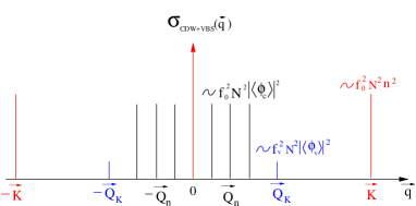
Figure 10: The characteristics of optical scattering cross section in the CDW+VBS phase in a triangular lattice. The $\vec{Q}_{n}$ stands for the three CDW ordering wavevectors $\vec{Q}_{\alpha}=2\pi/3(1,0),2\pi/3(0,1),2\pi/3(1,-1),\alpha=1,2,3$. Its magnitude is proportional to the CDW order parameter $|\langle\phi_{c}\rangle|^{2}$ in Eqn.67 and Eqn.88. The $\vec{Q}_{K}$ stands for the extra VBS ordering wavevector $\vec{Q}_{4}=2\pi/3(1,1)$. Its magnitude is proportional to the VBS order parameter $|\langle\phi_{v}\rangle|^{2}$ in Eqn.89. The ratio of the peak at $\vec{Q}_{n}$ over that at $\vec{K}$ is $\sim|\langle\phi_{c}\rangle^{2}/n^{2}\sim 1$, while the ratio of the peak at $\vec{Q}_{K}$ over that at $\vec{K}$ is $\sim|f_{a}/f_{0}|^{2}|\langle\phi_{v}\rangle|^{2}/n^{2}\sim 10^{-5}$. It should be visible in the current optical Bragg scattering experiments.

The SF to Mott transition in a triangular lattice can be similarly discussed as in Sec.V. The CDW ( CDW-VBS) to the CDW-SS ( CDW-VB-SS ) transition in a triangular lattice can also be similarly discussed as in Sec. V. However, it was shown in frus that there is no VB-SS in a frustrated lattice, the transition from a VBS to the SF can only be a direct first order, there is no an intervening VB-SS, so the Sect.VI does not apply to a frustrated lattice.

The generalization to non-Bravais lattices such the honeycomb, Kagome, Sutherland-Shastry and checkboard lattices frus ; frusrev can also be worked out similarly.

VIII Cavity QED detection method

Very recently, a non-destructive method off1 was proposed to detect Mott and superfluid phases by using cavity enhanced off-resonant light scattering from ultra-cold atoms loaded on optical lattices. In the off-resonant scattering, the atom-field detuning $\Delta$ is much larger than the atom-field coupling $g$ which, in turn, so the upper level of the atoms can be adiabatically eliminated. However, on the experimental side, the two cavities used in off1 are very hard to implement, on the theory side, all the concepts and calculations on quantum phases and phase transitions in off1 are not correct.

Because the cavity size in the experiment is $L_{cav}~{}175\mu m$ is so small, it is very difficult to manipulate experimentally the two cavities, so it is necessary to replace the pumping cavity in off1 by a strong classical laser beam in Fig.11a. However, the probing cavity is crucial to enhance the scattered photon mode $a$ along a given direction, then the experiments are much easier to implement. By using this workable experimental set-up, we will develop systematically a theory to detect the nature of quantum phases such as both the ground state and the excitation spectrum above the ground state of interacting bosons loaded in optical lattices. We explicitly show that off-resonant photons not only couple to the density order parameter, but also the valence bond order parameter due to the hopping of the bosons on the lattice. By tuning the angles between the classical laser beam and cavity photons, the photon characteristics such as quadrature in Eqn.4 ( to be measured by phase sensitive homedyne detection ) or one photon correlation functions in Eqn.7 ( to be measured by the Mach-Zehnder Interferometer (MZI) ) can detect not only the well known superfluid and Mott insulating phases, but also other interesting phases such as charge density wave (CDW), valence bond solid (VBS), CDW supersolid and VBS supersolid.

In the light scattering experiment Fig.1a, the light is scattered to any direction, so one has to use a small aperture to select the light scattered into a given direction $\vec{k}_{1}$. In this section, we propose to replace the aperture by a ring cavity ( Fig.11a ) to select a cavity photon mode, to enhance the scattered light and also select a given direction $\vec{k}_{1}$. In this section, we will show that by measuring the characteristics of the leaking photon out of the cavity, one can also determine the ground state and excitation spectrum of the atoms loaded in the optical lattice. So the experimental set-up in Fig.11 could be used as alternative to the light scattering experiment in Fig.1a

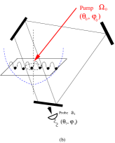
Figure 11: (a) The classical pump with a Rabi frequency $\Omega_{0}$ is shined on the 2 dimensional optical lattice at the angle $(\theta_{0},\phi_{0})$. A Ring cavity is used to enhance the scattered light $a$ at the angle $(\theta_{1},\phi_{1})$. Dashed ellipsis is a trap. Compare with the light scattering experiment Fig.1a. (b) Mach-Zehnder Interferometer scully to detect the single photon correlation function Eqn.78.

A non-destructive measurement is to probe the quantum phases formed by two level cold bosons by shining a classical laser beam with a Rabi frequency $\Omega$ and with a frequency $\omega_{0}$ far off the resonant frequency of the two level atoms $\omega_{a}$ and then measure the characteristics of scattered light $a$ from these quantum phases in a cavity with frequency $\omega_{c}$ ( Fig.11a ). The cavity will greatly enhance the scattering amplitude of the probe photons $a$. The boson Hamiltonian is given by Eqn.1. Assuming the mode functions $u_{l}(\vec{r})=e^{i\vec{k}_{l}\cdot\vec{r}_{i}+i\phi_{l}},l=0,1$ for the pump with the frequency $\omega_{0}$ and the traveling wave with the frequency $\omega_{1}=\omega_{c}$ in a ring cavity ( Fig.11b) where the two in-plane momenta of the two lights $\vec{k}_{0}=k_{0}\sin\theta_{0}(\cos\phi_{0},\sin\phi_{0}),\vec{k}_{1}=k_{1}\sin\theta_{1}(\cos\phi_{1},\sin\phi_{1})$. All the atoms are loaded in optical lattices formed by laser beams with wavevector $\vec{k}$. The pumping laser beam and the cavity photon $a$ are much weaker than the standing wave laser beams which form the optical lattices ( not shown in Fig.11 ). When it is far off the resonance, the light-atom detuning $\Delta_{la}=\omega_{l}-\omega_{a}$ is much larger than the Rabi frequency $\Omega_{0}$ which, in turn, is larger than $\kappa$ and $\gamma$, then after adiabatically eliminating the upper level of the two level atoms ( Fig.4 ), in the frame rotating with the pumping frequency $\omega_{0}$, the effective cavity QED Hamiltonian describing the interaction among the pumping laser, the off-resonant cavity photons and the ground level is:

$$H_{c} = (\omega_{c}-\omega_{0})a^{\dagger}a+\int d^{2}\vec{x}\Psi^{\dagger}(\vec{x})[\frac{\Omega^{2}_{0}}{\Delta_{0a}}+\frac{g^{2}}{\Delta_{0a}}a^{\dagger}a$$ (71)

$$+ \frac{g\Omega_{0}}{\Delta_{0a}}(a^{\dagger}e^{i(\vec{k}_{0}-\vec{k}_{1})\cdot\vec{r}}+h.c.)]\Psi(\vec{x})$$

Again, expanding the ground state atom field operator $\psi_{g}(\vec{r})=\sum_{i}b_{i}w(\vec{r}-\vec{r}_{i})$ in Eqn.30 where $w(\vec{r}-\vec{r}_{i})$ is the localized Wannier functions of the lowest Bloch band corresponding to $V_{OL}(\vec{r})$ and $b_{i}$ is the annihilation operator of an atom at the site $i$ in the Eqn.1, one get:

$$H_{c} = (\omega_{c}-\omega_{0}+\frac{g^{2}}{\Delta_{0a}}N_{at})a^{\dagger}a+\frac{\Omega^{2}_{0}}{\Delta_{0a}}N_{at}$$ (72)

$$+ \frac{g\Omega_{0}}{\Delta_{0a}}a^{\dagger}[\sum^{K}_{i}J_{i,i}n_{i}+\sum^{K}_{<ij>}J_{i,j}b^{\dagger}_{i}b_{j}]+h.c.$$

where the interacting matrix element is $J_{i,j}=\int d\vec{r}w(\vec{r}-\vec{r}_{i})u^{*}_{0}(\vec{r})u_{1}(\vec{r})w(\vec{r}-\vec{r}_{j})$.

It is very instructive to note the similarity and difference between Eqn.72 and Eqn.31. The incident light in Fig.1a and Fig.11 are the same, both are classical lights, but the classical scattered light is Fig.1a was replaced by the quantum cavity photon $a$ in Fig.11. So the scattered light Rabi frequency $\Omega$ in Eqn.31 is replaced by $ga^{\dagger}$ in Eqn.72 ( correspondingly, the scattered light in Fig.4 was replaced by the cavity photon $a$ ), the $e^{-i\omega t}$ in Eqn.31 was taken care of by the effective detuning of the cavity photon from the incident light $\Delta_{c}=\omega_{c}-\omega_{0}+\frac{g^{2}}{\Delta_{0a}}N_{at}$ in Eqn.72. In view of these similarity and differences, the $\hat{D}=\sum^{K}_{i}J_{i,i}n_{i}$ and $\hat{K}=\sum^{K}_{<ij>}J_{i,j}b^{\dagger}_{i}b_{j}$ in Eqn.72 can be very similarly manipulated as in Eqn.32 and 33 respectively.

In this section, we focus on the global illumination $K=N$ in Fig.11a. If there is a wedding cake structure inside a trap manybody ( see also Sec. XI ), then $K=N_{P}$ is the number of atoms in a given phase $P$ in the wedding cake. This can be more easily realized inside a flat trap flattrap or inside a harmonic trap with only one shell structure such as in Fig.12.

It is constructive to compare with the photon-exciton coupling $i\sum_{k}g(k)a^{\dagger}_{k}b_{\vec{k}}+h.c.$ in the electron-hole bilayer (EHBL) system short1 ; short2 ; excitonlong where photons couple to the SF order parameter $b_{\vec{k}}$ directly. Here the photons couple to both the density order parameter and also the valence bond order parameter instead of coupling to the SF order parameter directly. However, as shown in Eqn.8, inside the SF state, the density-density correlation function can also reflect the nature of SF precisely. So the coupling in Eqn.72 can reflect all the three orders: density order, valence bond order and SF order precisely.

The Heisenberg equation of motion for $a$ is:

$$\frac{da}{dt}=-i\Delta_{c}a-i\frac{\Omega_{0}g}{\Delta_{0a}}(\hat{D}+\hat{K})-\kappa a+F(t)$$ (73)

where $\Delta_{c}=\omega_{c}-\omega_{0}+\frac{g^{2}}{\Delta_{0a}}N_{at}$ stands for the effective detuning to the pumping frequency. The $F(t)$ is the noise operator satisfying: $\left\langle F^{\dagger}(t)F(t^{\prime})\right\rangle_{R}=\kappa\bar{n}_{\omega_{c}}\delta(t-t^{\prime}),\left\langle F(t)F^{\dagger}(t^{\prime})\right\rangle_{R}=\kappa(\bar{n}_{\omega_{c}}+1)\delta(t-t^{\prime}),\left\langle F(t)F(t^{\prime})\right\rangle_{R}=\left\langle F^{\dagger}(t)F^{\dagger}(t^{\prime})\right\rangle_{R}=0$ where the average $R$ is taken with respect to the reservoir, the $\bar{n}_{\omega_{c}}=1/(e^{\omega_{c}/T}-1)$ and $T$ is the temperature of the photon reservoir outside of the cavity.

(a) One time average: photon expectation value

The stationary solution for the Heisenberg equation of motion for $a$ Eqn.73 is:

$$\langle a\rangle=CN(\langle\hat{D}\rangle+\langle\hat{K}\rangle)$$ (74)

where the $C=-\frac{i\Omega_{0}g}{\Delta_{0a}(\kappa-i\Delta_{c})}$. The ensemble average $\langle\cdots\rangle$ is taken with respect to the initial state $|atom\rangle\times|0\rangle_{ph}$ where the $|atom\rangle$ stands for the ground state of interacting atoms in Eqn.1 and the $|0\rangle_{ph}$ stands for the initial zero photon state.

Substituting Eqn.32 and 33 into the Eqn.74 leads to

$$\langle a(\vec{q})\rangle=CN(\langle n(\vec{q})\rangle+f_{x}(\vec{q})\langle K_{x}(\vec{q})\rangle+f_{y}(\vec{q})\langle K_{y}(\vec{q})\rangle)$$ (75)

which can be measured by phase sensitive homedyne measurement scully ; short2 .

Again, we first look at the SF to Mott transition at integer fillings as discussed in Sect.V. Inside the SF, the $K_{i,i+\hat{x}}=K_{i,i+\hat{y}}$ is uniform which depends on $t-t_{c}$ in Fig.6, so at a reciprocal lattice $\vec{q}=\vec{K}$, Eqn.75 leads to:

$$\langle a(\vec{q})\rangle_{SF}-\langle a_{1}(\vec{q})\rangle_{Mott}=2CNf_{x}(\vec{q})K$$ (76)

which can be detected by phase sensitive homodyne detection scully ; short2 . It is an effective measurement of the kinetic energy inside the SF. This measurement can be contrasted to the increase of the scattering cross section from the Mott to the SF shown in Eqn.39 or from the CDW to CDW-SS, or from the VBS to VB-SS discussed in Section V-a and VI-a respectively.

(b) Two time averages: single photon correlation functions

Now we need to calculate the two-time one photon correlation function. The solution of Eqn.73 is eom :

$$a(t) = e^{-(\kappa+i\Delta_{c})(t-t_{0})}a(t_{0})$$ (77)

$$+ \int^{t}_{t_{0}}d\tau e^{-(\kappa+i\Delta_{c})(t-\tau)}(\eta_{a}(\tau)+F(\tau))$$

where $\eta_{a}(t)=-i\frac{\Omega_{0}g}{\Delta_{0a}}(\hat{D}(t)+\hat{K}(t))$ stands for the ”effective ” pumping force on $a$ from the atoms.

We observe the following three important facts: (1) If $t-t_{0}\gg 1/\kappa$, the first term drops out in the steady state. (2) The second term contributes significantly only when $t-\tau<1/\kappa$. It was known that in an optical lattice bloch ; boson , the hopping energy scale is much smaller than the cavity decay energy scale: $J\sim 10^{3}Hz\ll\kappa\sim 10^{7}Hz$, so we can approximate $\eta_{a}(\tau)\sim\eta_{a}(t)$ when $t-\tau<1/\kappa$. (3) In the optical cavity frequency regime $\hbar\omega_{c}\gg k_{B}T$, so $\bar{n}(\omega_{c})\sim 0$, then the noise term $F(t)$ drops out for a normal ordered correlation functions. The three facts lead to the two time photon correlation function:

$$\langle a^{\dagger}(\vec{q},t)a(\vec{q},0)\rangle = |C|^{2}[\langle D^{*}(\vec{q},t)D(\vec{q},0)\rangle$$ (78)

$$+ \langle K^{*}(\vec{q},t)K(\vec{q},0)\rangle]$$

where $\vec{q}=\vec{k}_{1}-\vec{k}_{0}$. We expect the crossing correlator $\langle D^{*}(\vec{q},t)K(\vec{q},0)\rangle$ is negligibly small in any phases. As shown in the Fig.11b, using the Mach-Zehnder Interferometer (MZI) scully and adjusting the difference between the two light paths, one can measure this two time one photon correlation function.

From Eqn.78, one can see that at any given momentum $\vec{q}$, the Florescence spectrum of the probing photons $I_{out}(\vec{q},\omega)=\int d\tau e^{-i\omega\tau}\langle a^{\dagger}(\vec{q},t+\tau)a(\vec{q},t)\rangle$ is :

$$I_{out}(\vec{q},\omega) = |C|^{2}N^{2}[|f_{0}(\vec{q})|^{2}S_{n}(\vec{q},\omega)$$ (79)

$$+ \sum_{\alpha=\hat{x},\hat{y}}|f_{\alpha}(\vec{q})|^{2}S_{K_{\alpha}}(\vec{q},\omega)]$$

which is similar to Eqn.35 or Eqn.90 after replacing $(\frac{\Omega^{2}}{\Delta})^{2}$ by $|C|^{2}$.

In Eqn.78, by setting $t=0$, one can see that the leaking photon number gives just the structure factor:

$$n_{ph}(\vec{q})=\langle a^{\dagger}(\vec{q})a(\vec{q})\rangle = |C|^{2}N^{2}[|f_{0}(\vec{q})|^{2}S_{n}(\vec{q})$$ (80)

$$+ \sum_{\alpha=\hat{x},\hat{y}}|f_{\alpha}(\vec{q})|^{2}S_{K_{\alpha}}(\vec{q})]$$

which is similar to Eqn.37 or Eqn.91 after replacing $(\frac{\Omega^{2}}{\Delta})^{2}$ by $|C|^{2}$. All the discussions in previous sections can also be applied here. For example, the scattering cross sections in a square lattice Fig.7 or in a triangular lattice Fig.10 should just be replaced by the photon numbers at the corresponding wavevectors. So we show that the Florescence spectrum of the leaking cavity photons can directly reflect the ground state and the excitation spectrum of any quantum state.

IX Quantum phases, phase transitions, Local density approximation and in situ measurements inside a harmonic trap

So far, we have been discussing the detections of quantum phases and phase transitions inside a flat trap. But most of the traps used in cold atom experiments are harmonic traps. Here we will discuss the effects of a harmonic trap. Inside a harmonic trap $V(r)=\frac{1}{2}\alpha r^{2}$ where the $\alpha$ is the curvature, one can construct the length scale curvature :

$$L_{c}\sim(\alpha/t)^{-1/2}$$ (81)

where the $t$ is the hopping in Eqn.1. As shown in curvature , it plays a similar role as a finite size $L$ in the homogeneous system.

In cold atom experiments inside a harmonic trap, it is more convenient to express the scaling functions in Eqn.29 in terms of the finite temperature $T$ :

$$S_{n}(\vec{Q}_{N},i\omega_{n}=0) = T^{d-2+\eta}F_{ns}(\frac{K-K_{c}}{T^{1/\nu z}},\beta/L^{z}_{c})$$

$$S_{n}(\vec{Q}_{N},\tau=0) = T^{\frac{2\beta}{z\nu}}F_{ne}(\frac{K-K_{c}}{T^{1/\nu z}},\beta/L^{z}_{c})$$ (82)

The Local density approximation (LDA) means that the system’s properties at the local chemical potential $\mu(r)=\mu-V(r)$ can reflect those of a homogeneous system at this local $\mu(r)$. Then determining the bulk thermodynamic quantities as a function of the chemical potential corresponds to determining the $r$ dependence in the harmonic trap trapthe0 ; trapthe1 . We expect that the LDA works in the $1/T<L_{c}$ limit, so the trapped system feels the temperature effects before it feels the curvature effects of the trap. In all the present experiments, the $T\sim 20nK$, so $1/T$ is indeed smaller than the $L_{c}$, so the system feels the temperature effects before it feels the curvature effects, the LDA is valid. Then the tuning parameter $K$ in Eqn.82 can be taken as the local chemical potential $\mu(r)=\mu-V(r)$. Setting $K=\mu(r)$ and $\beta/L^{z}_{c}\rightarrow 0$ in Eqn.82 and lead to:

$$S^{LDA}_{n}(\vec{Q}_{N},i\omega_{n}=0) = T^{d-2+\eta}F_{ns}(\frac{\mu-\mu_{c}}{T^{1/\nu z}})$$

$$S^{LDA}_{n}(\vec{Q}_{N},\tau=0) = T^{\frac{2\beta}{z\nu}}F_{ne}(\frac{\mu-\mu_{c}}{T^{1/\nu z}})$$ (83)

Note that we expect that the scaling functions will eventually break down at lower temperatures where the system starts to feel the curvature effects of the trap.

Another important effect of the trap is that there exist multiple phases inside an harmonic trap curvature . As the local chemical potential $\mu(r)=\mu-V(r)$ decreasing from the center of the trap to the boundary, there is always a shell structure of phases inside a trap. For example, at filling $n=1$, there is a Mott phase at the center, then there is always a SF shell around the boundary ( Fig.12 ). So there is a Mott gap in the center, gapless SF around the boundary. To some extent, this is similar to quantum Hall state where there is a gap in the bulk, but gapless edge state along the boundary. But the main difference is that here there is a harmonic trap, while in Quantum Hall system, there is a sharp sample edge within a few magnetic length.

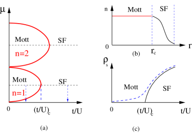
Figure 12: (a) The zero temperature phase diagram of a homogeneous short-ranged boson Hubbard model boson . See Fig.6 for its finite temperature phase diagram. Inside a trap, the local chemical potential $\mu(r)=\mu-\frac{1}{2}Kr^{2}$ decreases from the center to the boundary. Under the LDA, there is a Mott to SF transition at $r=r_{c}$. (b) The well-known shell structure of Mott state in the center and the SF in the boundary (c) The red solid line is the superfluid density in a homogeneous system with $\rho_{s}\sim(t-t_{c})^{\nu}$. The blue dashed line is inside a trap

Under the LDA, there is a Mott to SF transition in Fig.12b at $r=r_{c}$, one can apply the thermodynamic scaling Eqn.59 and Eqn.60 as:

$$\rho_{s}(r) \sim \delta n(r)=1-n(r)$$ (84)

$$= \frac{m_{a}a^{2}\delta\mu(r)}{4\pi\hbar^{2}}\ln[\frac{\hbar^{2}}{2m_{a}a^{2}\delta\mu(r)}]$$

where $\delta\mu(r)=\mu_{c}-\mu(r)=\frac{1}{2}K(r^{2}-r^{2}_{c})\sim r-r_{c}$. In principal, this scaling relation can be tested by the in situ measurement in insitu0 ; insitu1 . However, it remains challenging to measure the dynamic density-density correlation function Eqn.61 by the in situ meathod. It seems only the three scattering experiments can measure the dynamic correlations. So the in situ measurement and the three scattering measurements are complimentary to each other.

Under the Local density approximation (LDA), a scaling analysis can be written down across the 2d Kosterlitz-Thouless (KT) superfluid to normal gas transition from the center of the trap to the boundary. The KT transition is a finite temperature transition at $T=T_{c}$, the correlation length $\xi\sim e^{1/\sqrt{T-T_{c}}}$. Indeed, the recent in situ measurements insitu1 on local density and local density fluctuations were performed to confirm the scaling functions at different temperatures and different interaction strengths.

There are many possible ways to observe a stabilized supersolid in a cold atom experiment. One possible route is to using the shell structure inside a harmonic trap. For hard core bosons, it was shown by the QMC in square , the $(\pi,\pi)$ X-CDW SS is not stable against phase separation with $V_{1}>0,V_{2}=0$, but the $(\pi,0)$ stripe SS may be stable with $V_{1}=0,V_{2}>0$. The transition from the stripe SS to the SF is a first order transition. However, for hard core bosons with a dipole-dipole interaction, the $(\pi,\pi)$ ( $\vec{Q}_{n}=2\pi/3(1,1)$ in Fig. 14a ) X-CDW supersolid was found to be stable in a square ( triangular ) lattice dipolarss ; dipolarsstri in a large parameter regimes near the half filling int . Furthermore, it was found the CDW-SS to the SF transition is a second order transition in the $3d$ Ising universality class. Now if we take a half filling at the center of the trap, so it is a X-CDW at the center, a SF near the boundary, then there could be a stable vacancy-like X-CDW supersolid bipart ; frus separating the X-CDW from the SF ( Fig.13b ). This is a ring structure with a periodic boundary condition around the center, so it may be favorable to stabilize this X-CDW SS in the quasi-1d ring structure. Indeed, a SS was found to be stable in 1d optical lattice in sca . Under the LDA, the transition at $r_{c1}$ is a second order in the universality class of the Mott to the SF transition with $z=2,\nu=1/2,\eta=0$ in Fig. 12. Then Eqn.84 still holds with $\delta n(r)=1/2-n(r)$. The transition at $r_{c2}$ is also a second order in the universality class of the 3d Ising class with $z=1,1/\nu=1.594,2\beta/\nu=1.037$. Then we can write Eqn.83 as

$$S^{LDA}_{n}(\vec{Q}_{N},\tau=0)=T^{1.037}F_{ne}(\frac{\mu-\mu_{c}}{T^{1.594}})$$ (85)

which can be tested by the combination of in situ measurements and the scattering measurements.

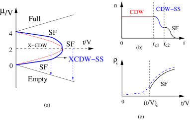
Figure 13: (a) The zero temperature phase diagram of a homogeneous boson Hubbard model with dipole-dipole interaction strength $V$ dipolarss ; dipolarsstri . Comparing with the Fig.3. (b) The shell structure of X-CDW state in the center and the SF in the boundary with the CDW-SS intervening between the two. The 2nd order transitions at $r_{c1}$ and $r_{c2}$ are discussed in the text. (c) The transition from the X-CDW to the SF is not studied yet. It is likely to be a first order transition. Then the red solid line is the superfluid density in a homogeneous system with $\rho_{s}$ jump discontinuously at the CDW-SF transition. The blue dashed line is inside a trap

X Conclusions

Due to the dilutees and charge neutral of cold atoms, the experimental ways to detect possible quantum phases and quantum phase transitions of cold atoms in optical lattices in a minimum destructive way remain very limited. In this paper, we developed a systematic and unified theory to use the three different experiments: optical Bragg scattering, atom Bragg spectroscopy or off-resonant cavity enhanced scattering to detect the ground states, the elementary excitation spectra and the corresponding spectral weights of many quantum phases in both bipartite and frustrated lattices. We show that the two photon Raman processes in all the three measurements not only couple to the density order parameter, but also the valence bond order parameter due to the hopping of the bosons on the lattice. This coupling to the VBS order is extremely sensitive to the superfluid order or VBS order at corresponding ordering wavevectors. It is this coupling which make the three experiments being able to detect not only the well known SF and Mott phases, but also many other important phases such as CDW, VBS, CDW-VBS and all kinds of supersolids. The first experiment braggbog ; braggeng was well established, the secondbraggafm ; blochlight is being performed in several experimental groups, the third is a possible new experimental set-up complementary to the first two. The combinations of the three can be used as powerful and complete tools to study the properties of many quantum phases of atoms in optical lattices.

The physical measurable quantities of the three experiments are the light scattering cross sections, the atom scattered clouds and the cavity leaking photons respectively. All these experimental measurable quantities are determined by the density-density and bond-bond correlation functions. From symmetry points of view, we analyzed several general properties of the density-density and bond-bond correlation functions in both bipartite and frustrated lattices. The CDW and VBS order parameters in bipartite lattices are Ising order parameter $m$ and $K$ respectively, while those in frustrated lattices are complex $U(1)$ order parameter $\phi_{c}$ and $\phi_{v}$ respectively. This difference leads to several new features of light scattering cross section in frustrated lattices. Previous literatures in quantum phase transitions focused on computing order parameter correlation functions. Here, motivated by the fact that all the three experimental inelastic scattering only couples to the density-density correlation function instead of coupling to the order parameter directly, we computed the density-density correlation function in the Mott phase, Superfluid phase and the quantum critical regime in both $z=1$ and the $z=2$ universality class in Fig.6 and Fig.9 respectively.

At integer fillings, when $\vec{q}$ matches a reciprocal lattice vector $\vec{K}$ of the underlying OL, there is a increase in the optical scattering cross section as the system evolves from the Mott to the SF state. This increase may be used as an effective measure of the average kinetic energy inside the SF. At half integer fillings, in the CDW state, when $\vec{q}$ matches the CDW ordering wavevector $\vec{Q}_{n}$ and $\vec{K}$, there is a diffraction peak proportional to the CDW order parameter squared and the density squared respectively (Fig.7a), the ratio of the two peaks are good measure of the CDW order parameter. In the VBS state, when $\vec{q}$ matches the VBS ordering wavevector $\vec{Q}_{K}$, there is a much smaller, but detectable diffraction peak proportional to the VBS order parameter squared, when it matches $\vec{K}$, there is also a diffraction peak proportional to the uniform density in the VBS state (Fig.7b). The ratio of the two peaks are good measure of the VBS order parameter. All the diffraction peaks scale as the square of the numbers of atoms inside the trap. All these characteristics can determine uniquely CDW and VBS state at commensurate fillings and the corresponding CDW supersolid and VBS supersolid slightly away from the commensurate fillings. In a frustrated lattice such as a triangular lattice, there are a new kind phase with both CDW and VBS orders called CDW+VBS phase in Fig.15. There are corresponding several new features in the light scattering cross sections. We also describe how it can detect both the CDW order $|\langle\phi_{c}\rangle|^{2}$ and the VBS order $|\langle\phi_{v}\rangle|^{2}$ in the CDW-VBS phase in Fig.10. We also point out that due to the smallness of the CDW gap and even smaller VBS gap compared to the energy of the incident light, the tiny energy difference $\delta E=E_{f}-E_{i}$ could be detected by quantum beats in phase sensitive homodyne interference experiments. The superfluid components in the CDW and VBS supersolids can be determined by the momentum braggbog transfer Bragg spectroscopy. While the excitation gaps in the CDW and VBS and corresponding spectral weights can be detected by the energy transfer braggeng Bragg spectroscopy. So the combinations of these photon and atom scatterings can be used to detect many conventional and exotic quantum phases and their excitation spectra of cold atoms in optical lattices as soon as these phases are within experimental reach.

We also propose the cavity QED as another possible effective detection method. It is constructive to compare Fig.11 with the very recent experiments to realize the $Z_{2}$ super-radiant phase orbital and to realize all kinds of bi-stabilities in BEC, BEC spinor, fermion or spin-orbit coupled systemsqedbecoff ; spinor ; fermion ; spinorbit . In the super-radiant experiment orbital , the pumping is a transverse pumping similar to that in Fig.11. The system is in a good cavity limit, so the Hamiltonian dynamics dominates over any dissipation process. As the transverse pumping power increases above a critical value, the system will evolve from a normal phase into a super-radiant phase. So the pumping laser is used to induce the dramatic change of the ground state through the Raman transition. The change of the ground state and the collective excitation spectrum of the strongly coupled atom-photon system can be detected by the Florescence spectrum. In the bi-stability experiments qedbecoff ; spinor ; fermion ; spinorbit , the pumping is a longitudinal pumping, so it pumps the cavity photon directly, no Raman process in Fig.4 is involved. As the longitudinal pumping power increases above a critical value, the system will suffer bi-instabilities, even tri-stabilities spinorbit . So the pumping laser is also used to change the properties of the strongly coupled photon-atom system by non-linear effects which can be detected by cavity transmission spectrum. The system is in a bad cavity limit. In both cases, the pumping is strong which induces highly non-linear optical and matter effects. The approximation is a two level matter wave approximation which is justified in the strong pumping case. However, in the present cavity QED detection scheme in Fig. 11, the classical laser is used to just probe the quantum phases of the cold atoms so that it will not disturb the properties of the system itself. The cavity is in the bad cavity limit. The approximation we made is a linear response theory which is justified in the weak pumping regime. But we treat all the matter modes exactly which are what one like to detect by the Florescence spectrum. Furthermore, the cavity QED detection does not involve the TOF measurements, so it is non-destructive. However, putting OL inside a ring cavity shown in Fig. 11 may still present serious experimental challenges.

The local density and local density fluctuations can be directly measured by recently advanced in situ spatially resolved imagings. In the temperature regime where the LDA holds, the Mott to SF transition can be directly probed across the shell structure inside a harmonic trap. The CDW to the CDW-SS and then the CDW-SS to the SF transition can also be directly probed across the multi-shells structure inside a harmonic trap. The two kinds of measurement are complementary and dual to each other. The combination of both class of detection methods could be used to match the combination of STM, the ARPES and neutron scatterings in condensed matter systems, therefore achieve the putative goals of quantum simulations of quantum phases and quantum phase transition.

Acknowledgements

We thank I. Bloch, Jason Ho, R.Hulet, Juan Pino, R. Scalettar and Han Pu for very helpful discussions. J. Ye also thanks Jason Ho, A. V. Balatsky and Han Pu for their hospitalities during his visit at Ohio state university, the LANL and Rice university where part of this work is done. J. Ye’s research is supported by NSF-DMR-1161497, NSFC-11074173, Beijing Municipal Commission of Education under grant No.PHR201107121, at KITP is supported in part by the NSF under grant No. PHY-1125915. YC was supported by NSFC-10874032 and 11074043, the State Key Programs of China (Grant no. 2009CB929204) and Shanghai Municipal Government. W.P. Zhang’s research was supported by the National Basic Research Program of China (973 Program) under Grant No.2011CB921604, and NSFC under Grant Nos.10588402 and 10474055.

Appendix A Review of quantum phases in bipartite and frustrated lattices

Quantum phases of the Extended Boson Hubbard Model (EBHM) with long range interactions in Eqn.1 are thoroughly studied by various analytic and numerical methods such as the spin wave expansion in Ref.gan , the dual vortex method (DVM) in Refs.pq1 ; mob ; bipart ; frus and quantum Monte-Carlo simulations in Refs.square ; squaresoft ; frusqmc ; sandvik ; honey . In the following, we review some interesting quantum phases in bipartite and frustrated lattices respectively. This appendix is not new, but pave the way for the discussions on the detections of these quantum phases in the main text.

A.1 Some Quantum phases in bipartite optical lattices

Some of the important Mott insulating phases at commensurate fillings in a square lattice were already summarized in the Fig.2. Some quantum phases, especially supersolid phases and quantum phase transitions slightly away from commensurate fillings are studied by the DVM in mob ; bipart ; frus . The zero temperature phase diagrams of the chemical potential $\mu$ against the quantum fluctuations $t/V_{1}$ slightly away from $1/2$ fillings are shown in the Fig.3. The DVM is a symmetry based approach, so the results achieved from the DVM can be compared to any microscopic models. For example, it can be compared to $V_{1},V_{2},....$ model, or to the dipole-dipole interaction model. If the supersolid phases are stable or not depend on the specific microscopic interactions. As said in Sect.II-D, the dipole-dipole interaction is particularly favorable to the formation of CDW supersolids slightly away $1/2$ fillings.

In a honeycomb lattice, we can also find some CDW and VBS phases bipart ; frus . Because of their similarity to the quantum phases in a square lattice, we will not discuss the honeycomb lattice specifically.

A.2 Some Quantum phases in frustrated optical lattices

In a triangular lattice at the filling factor $f=1/3$, it is easy to see a CDW phase and a triangular Valence bond ( TVB ) phase frus .

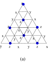
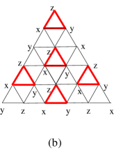
Figure 14: Several insulating states at filling factor $f=1/3$ in a triangular lattice (a) the X-CDW at $\vec{Q}_{n}=2\pi/3(1,1)$ (b) VBS at $\vec{Q}_{K}=2\pi/3(1,1)$. See gan ; frus .

The density in the X-CDW Fig.14a is:

$$\rho(\vec{r})=A\cos\vec{Q}_{n}\cdot\vec{r}+1/3$$ (86)

where $\vec{Q}_{n}=2\pi/3(1,1)$. Putting $\vec{r}\rightarrow\vec{r}-\vec{a}_{1},\vec{r}\rightarrow\vec{r}-\vec{a}_{2}$ will correspond to the other two X-CDW located at the other two sublattices.

If $\vec{Q}_{n}=2\pi/3(1,0),2\pi/3(0,1),2\pi/3(1,-1)$, then Eqn.86 stands for a stripe phase along $\vec{a}_{1},\vec{a}_{2},\vec{a}_{3}$ respectively. For hard core bosons with a dipole-dipole interaction, this X-CDW at $f=1/3$ and the X-CDW supersolid slightly away from $f=1/3$ was found to be stable in a large parameter regimes in a triangular lattice dipolarss .

The triangular VB state in Fig.14b is:

$$B_{1}(\vec{r}) = K_{1}\cos\vec{Q}_{K}\cdot\vec{r}+K_{2}$$

$$B_{d}(\vec{r}) = K_{1}\cos\vec{Q}_{K}\cdot\vec{r}+K_{2}$$

$$B_{2}(\vec{r}) = K_{1}\cos(\vec{Q}_{K}\cdot\vec{r}-\frac{2\pi}{3})+K_{2}$$ (87)

where $\vec{Q}_{K}=2\pi/3(1,1)$ and the $B_{1}(\vec{r}),B_{d}(\vec{r}),B_{2}(\vec{r})$ are the three bonds along the 3 directions along $\vec{a}_{1},\vec{a}_{d},\vec{a}_{2}$. One can see that $B_{2}(\vec{r})=B_{1}(\vec{r}-\vec{a}_{1})$ as expected from the symmetry breaking patterns in Fig.14b.

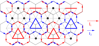
Figure 15: The CDW-VB phase in a triangular lattice at $f=1/3$ in the easy plane limit $v<0,w>0$. The $(0,0)$ sets the origin of the direct triangular lattice. There are two different vortex currents flowing in the dual honeycomb lattice. The red current is $I_{1}=\sin\frac{3\pi}{9}+\sin\frac{2\pi}{9}$, the blue current $I_{2}=\sin\frac{\pi}{9}+\sin\frac{2\pi}{9}$. The two different currents indicate 3 boson different densities in the direct triangular lattice. The density and bond distributions are given in Eqn.88 and Eqn.89 respectively. See frus .

In a triangular lattice, we also identify a phase with both CDW and VBS order in Fig.15 frus . The CDW order in the CDW+VBS phase is given by:

$$\rho_{CV}(\vec{x}) = 1/3+4\delta\sqrt{\frac{I^{2}_{1}-I_{1}I_{2}+I^{2}_{2}}{3}}[-\cos(\frac{2\pi}{3}x+\frac{5\pi}{18})$$ (88)

$$+ \cos(\frac{2\pi}{3}y+\frac{\pi}{18})+\cos(\frac{2\pi}{3}(x-y)+\frac{\pi}{18})]$$

where $\delta$ is the CDW order parameter and $I_{1},I_{2}$ are the vortex currents in Fig.15.

The VBS order in the CDW+VBS phase is given by:

$$B_{1}(\vec{x}) = B_{d}(\vec{x})=c\delta(I_{1}+I_{2})(1+2\cos\frac{2\pi}{3}(x+y))$$

$$+ 2c\delta\sqrt{I^{2}_{1}-I_{1}I_{2}+I^{2}_{2}}[\cos(\frac{2\pi}{3}x+\frac{2\pi}{9})$$

$$+ \cos(\frac{2\pi}{3}y-\frac{2\pi}{9})+\cos(\frac{2\pi}{3}(x-y)-\frac{2\pi}{9})]$$

$$B_{2}(\vec{x}) = c\delta(I_{1}+I_{2})(1+2\cos[\frac{2\pi}{3}(x+y)-\frac{2\pi}{3}])$$ (89)

$$+ 2c\delta\sqrt{I^{2}_{1}-I_{1}I_{2}+I^{2}_{2}}[\cos(\frac{2\pi}{3}x-\frac{4\pi}{9})$$

$$+ \cos(\frac{2\pi}{3}y-\frac{2\pi}{9})+\cos(\frac{2\pi}{3}(x-y)-\frac{8\pi}{9})]$$

where the $c$ is an unknown constant. One can see that $B_{2}(\vec{x})=B_{1}(\vec{x}-\vec{a}_{1})$ as expected from the symmetry breaking patterns in Fig.15.

When comparing with the CDW order in Eqn.88, we can see that in addition to the 3 ordering wave vectors $\vec{Q}_{\alpha}=2\pi/3(1,0),2\pi/3(0,1),2\pi/3(1,-1),\alpha=1,2,3$, there is also a new VBS ordering wave vector $\vec{Q}_{4}=2\pi/3(1,1)$. It is this new ordering wave vector which makes the detection of the VBS order inside the CDW-VB phase possible to be discussed in Sec.VI.

In a Kagome lattice, we also found some interesting CDW, VBS and CDW+VBS phase frus . Because of their similarity to the quantum phases in a triangular lattice, we will not discuss the Kagome lattice specifically.

Appendix B Photon Bragg scattering experiments

The main difference of light scattering in cold atom systems from that in condensed matter system is that the former is charge neutral, so the off-resonant Ramon scattering processes in Fig.4 are involved, what are measured are the density-density and bond-bond correlation functions listed in Eqn.35. While in the latter, the ions carry electric charges, so there is a direct scattering. So the latter usually has a much bigger scattering cross sections. For example, in high $T_{c}$ superconductors hightc , the ARPES directly measures the single quasi-particle spectral weights.

In the previous sections, we showed that the elastic photon Bragg scattering can not only detect the CDW ordering at $\vec{q}=\vec{Q}_{n}$ easily ( Fig.7a ), but also be used to detect the VBS ordering at $\vec{q}=\vec{Q}_{K}$( Fig.7b ). It is also quite sensitive to the small superfluid component in the CDW-SS and VB-SS. We also showed that the photon Bragg scattering cross section increases from the Mott to the SF phase due to the boson flow through the whole optical lattice inside the SF phase. So this detection method is especially powerful to detect the ground states of various quantum phases. But it may not be easy to detect the excitation spectrum by using this method due to the following reasons: Due to the smallness of the CDW gap $\Delta_{CDW}\sim U\sim 10kHz\sim 1\mu K$ and even smaller VBS gap $\Delta_{VBS}\sim t^{2}/U\sim nK$ compared to the energy of the incident light $E_{i}\sim 10^{5}GHz$, the tiny energy difference $\delta E=E_{f}-E_{i}$ is not easy be detected in the present inelastic Bragg scattering experiments. So far, all the previous Bragg scattering experiments braggsingle only focused on the elastic scattering with $\omega=0$ which detect the static orders of OL itself. However, it was argued braggsingle that the integrated in-elastic scattering can be used to detect the temperature of cold atoms in OL with incident light intensity $I_{in}\sim 500\mu W/cm^{2}$ and the detuning in Fig.4 $\Delta\sim 20\gamma$ where $\gamma$ is the linewidth of the excited state. We expect that the tiny energy difference is still detectable by measuring the quantum beats of phase sensitive homodyne interference experiments. So the possible future combination of the light scattering in Fig.1a combined with the quantum beat measurement can be used to detect not only the ground state, but also the excitation spectrum. Note that in contrast to the atom Bragg spectroscopy to be discussed in the following appendix, the photon Bragg spectroscopy does not involve the TOF measurements, so it is a non-destructive measurement.

Appendix C Atom Bragg scattering experiments

There are also two different Atom Bragg scattering experiments. The Momentum Bragg spectroscopy is more applicable in the superfluid side to detect its Bogoliubov excitations. While the energy Bragg spectroscopy is more applicable in the insulating side to detect its excitation gap. But it may not be as effective as the photon Bragg scattering to detect the ground states of the quantum phases.

(a) Momentum Bragg spectroscopy

It measures the atom diffraction from the light gratings formed by the two laser beams in Fig.1b, so it is a complementary ( or dual ) to the light scattering which measures the light diffraction from the atoms gratings. It is used to measure the Bogoliubov excitation spectrum inside a superfluid.

The main experimental procedures of the Momentum Bragg spectroscopy braggbog are: (1) The duration of the two incident light pulses in Fig.1b is about $\tau_{p}\sim 400\mu s$, then shut off ( Fig.16 a). (2) Then the optical lattices and also the trap in Fig.1b are released shortly after the turn-off of the light pulse. (3) Then after some expanding time $\tau_{exp}\sim 200\tau_{p}\sim 8ms$, the time of flight images are taken to measure the momentum distribution of the expanding gas. During the expansion process, the energy and momentum of the elementary excitations are transferred to the free particles.

Only when the imparted energy $\omega$ and the imparted momentum $\vec{k}$ match the dispersion relation of the elementary excitations in the system, one can observe a scattered cloud ( Fig.16 b) whose number $N_{sc}(\vec{q},\omega)$ is proportional to the dynamic structure factor:

$$N_{sc}(\vec{q},\omega) \sim (\frac{\Omega^{2}}{\Delta})^{2}N^{2}[|f_{0}(\vec{q})|^{2}S_{n}(\vec{q},\omega)$$ (90)

$$+ \sum_{\alpha=\hat{x},\hat{y}}|f_{\alpha}(\vec{q})|^{2}S_{K_{\alpha}}(\vec{q},\omega)]$$

where the prefactor is proportional to the duration $\tau_{p}$, the incident density $I_{in}\sim 1mW/cm^{2}$ in Fig.16. When comparing with Eqn.35, one can see that the scattering cross section in the light scattering experiment is replaced by the scattered clouds in the atom Bragg spectroscopy.

The integrated scattered atoms $N_{sc}(\vec{q})=\int d\omega N_{sc}(\vec{q},\omega)$ is proportional to the equal-time response function

$$N_{sc}(\vec{q}) \sim (\frac{\Omega^{2}}{\Delta})^{2}N^{2}[|f_{0}(\vec{q})|^{2}S_{n}(\vec{q})$$ (91)

$$+ \sum_{\alpha=\hat{x},\hat{y}}|f_{\alpha}(\vec{q})|^{2}S_{K_{\alpha}}(\vec{q})]$$

This can be measured by scanning the frequency $\omega$ at fixed $\vec{q}$. For the current experimental pulse duration time and the incident density, the scattered atoms around $\vec{q}$ are about $10-20\%$ of the condensate atoms around $\vec{q}=0$: $N_{sc}(\vec{q})/N_{0}(\vec{q}=0)\sim 0.1-0.2$. Then one may neglect nonlinear terms at the required laser powers. Possible spontaneous scattering processes can also be suppressed. In real atom Bragg spectroscopy experiments, there are several technical issues such as the signal strength, the geometry dependence, the suppressions of the multi-photon processes and super-radiance… need to be considered, but the basic picture is presented in this section and sketched in the Fig.16.

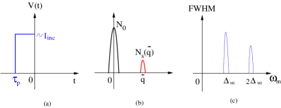
Figure 16: (a) The duration and strength of the two laser beams in the atom Bragg spectroscopy in Fig.1b. (b) In the momentum transfer Bragg spectroscopy, the scattered atom cloud at $\vec{q}$ verses the condensate cloud at $\vec{q}=0$. In a TOF image, the momentum is mapped to the axial distance $z$. So the two peaks are separated by a distance in the axial direction. (c) In the energy Bragg spectroscopy, the full width at half maximum (FWHM ) of the central peak in the TOF image peaks when the modulation frequency $\omega_{m}$ matches the Mott gap $\Delta_{Mott}$ in the Mott insulating phase. The momentum is fixed at $\vec{q}=0$ in the Mott state, but can be tuned to $\vec{Q}_{n}$ or $\vec{Q}_{K}$ in a CDW or VBS state to measure $\Delta_{CDW}$ and $\Delta_{VBS}$ respectively.

(b) Energy Bragg spectroscopy

The excitation gaps in the Mott, CDW or VBS and corresponding spectral weights in Fig.8 can be detected by the energy transfer Bragg spectroscopy braggeng . In this experiment, the two laser beams in Fig.1b is counter-propagating, so simply super-imposed on the external laser beams forming the optical lattice: $V_{OL}(x,t)=(V_{OL,0}(x,t)+A_{m}\sin\omega_{m}t)\cos^{2}kx$. The modulation $A_{m}$ and the frequency difference $\omega_{m}$ introduces two sidebands with frequencies $\pm\omega_{m}$ relative to the OL laser frequency. So when the imparted energy $\omega_{m}$ matches the excitation gap $\Delta$ at $\vec{q}=0$ or any reciprocal lattice vector $\vec{K}$ inside the Mott state, there is a maximum response of the atoms. After the excitation, the OL potential is ramping down linearly to the SF regime and kept in this shallow potential for some time. Then the trap in Fig.1b is suddenly switched off, the atoms’ interference images are taken after their $20ms$ ballistic expansion. The full width at half maximum (FWHM) of the central peak is taken as the measure of the energy deposited in the atom clouds by the excitation. Namely, the FWHM represents the system’s repones to the two laser beams in Fig.1b. Indeed, discrete peaks in the FWHM were observed braggeng at discrete spectrum $\omega_{m}=n\Delta_{MI},n=0,\pm 1,\cdots$ in Fig.16c.

Note that the gaps inside the CDW, VBS, CDW-VBS and the corresponding supersolids in Fig.8 are at momentum $\vec{q}=\vec{Q}_{n}$ or $\vec{q}=\vec{Q}_{K}$. We expect similar energy transfer Bragg spectroscopy can be used to measure these gaps when one tune $\vec{q}=\vec{Q}_{n}$ or $\vec{q}=\vec{Q}_{K}$ in Fig.1b and Fig.16c. The corresponding spectral weights are just the areas under the peaks in Fig.16c.

It maybe useful to make a brief comparison between the atom and photon Bragg scattering here, the photon Bragg scattering is very good for detecting the orders, it also does not involve the TOF measurements, so it is a non-destructive measurement. As explained in the previous section, so far, it is very challenging, but still possible to measure the excitation spectrum by using very precise quantum beating interference measurements. However, as discussed in this section, the atom Bragg spectroscopy is not very suitable to detect the ground state orders, especially all the possible insulating states, but very effective to detect the excitation spectra. For example, the superfluid components in the CDW and VBS supersolids can be determined by the momentum braggbog transfer Bragg spectroscopy. The gaps in the CDW and VBS supersolids can be measured by the energy braggeng transfer Bragg spectroscopy. Because the atom Bragg spectroscopy involves the TOF measurements, so it is a destructive measurement. So the photon and atom Bragg spectroscopy are two complementary detection methods, the combinations of both can be used to detect many conventional and exotic quantum phases and their excitation spectra of cold atoms in optical lattices as soon as these phases are within experimental reach.

Appendix D Superfluid stiffness and QED detection at the 2 dimensional classical diffraction minima $\vec{q}=(\pi,\pi)$.

The Cavity QED scattering from the SF and Mott phase at 1d near $q=\pi$ was addressed in off1 . Particularly, they discussed the cavity QED scattering from the Mott and the SF phase at the geometry to suppress the classical diffraction. In this geometry, $\theta_{0}=0,\theta_{1}=\pi/2$ in Fig.11a, so $\hat{D}=\sum_{i}(-1)^{i}n_{i}$, so $\langle a^{\dagger}_{1}a_{1}\rangle_{MI}=0$ in the $t/U\rightarrow 0$ limit in Fig.6 ( see below Eqn.94 ). In Ref.off1 , the SF ground state was taken as a non-interacting BEC state $|BEC\rangle_{non}\sim(\sum_{i}b^{\dagger}_{i})^{N}|0\rangle$, so the results in off1 on the SF side are based on the fact that the non-local pair correlation functions between the atom numbers at different sites $\langle n_{i}n_{j}\rangle$ in the non-interacting BEC state are the same for any $i\neq j$. This infinite long-range correlation is certainly not valid in any SF, so their photon spectrum on the SF side are in-correct. In this appendix, we will calculate the photon number spectrum inside the SF phase and show that it is an effective measure of the superfluid density $\rho_{s}$ and the phonon velocity $v$ of the SF. While the two fundamental physical quantities for the SF are not even defined for the non-interacting BEC state.

It is well known that a non-interacting BEC state is a pathological state. A repulsive interaction is needed to transform the BEC state to a SF state and leads to the gapless Goldstone mode above the SF ground state shown in Eqn.8 and in Fig.8. The Fourier transform of the equal density-density correlation function in Eqn.10 at $d=2$ is:

$$\langle\delta n_{i}\delta n_{j}\rangle_{SF}=\langle n_{i}n_{j}\rangle-n^{2}\sim\rho_{s}/v|i-j|^{3}$$ (92)

which decays as a power law as the distance between the two sites $|i-j|\gg a$ due to the gapless Goldstone mode in the SF and also depends on the superfluid density $\rho_{s}$ and the Goldstone mode velocity $v$. Strictly speaking, Eqn.92 only holds at very long distance $|i-j|\gg a$, for example, it certainly breaks down at $i=j$, but we expect $\langle n^{2}_{i}\rangle_{SF}-n^{2}\sim\rho_{s}/v$ still holds. In contrast, from Eqn.11, inside the Mott state

$$\langle\delta n_{i}\delta n_{j}\rangle_{MI}=\langle n_{i}n_{j}\rangle-n^{2}\sim e^{-|i-j|/\xi_{MI}}$$ (93)

where $\xi_{MI}\sim 1/\Delta_{MI}$ is the correlation length inside the Mott state. This equation is consistent with Eqn.42 in the momentum space in the Mott phase.

While at the QCP between the SF to Mott transition in Fig.6, because $\delta n$ is a conserved quantity, so no anomalous dimension, then we have:

$$\langle\delta n_{i}\delta n_{j}\rangle_{QC}=\langle n_{i}n_{j}\rangle-n^{2}\sim 1/|i-j|^{4}$$ (94)

for $|i-j|\gg a$. This equation is consistent with Eqn.47 in the momentum space at the QC.

Then from Eqn.78, we can see that at $\vec{q}=(\pi,\pi)$, the photon number is $\langle a^{\dagger}(\vec{q},0)a(\vec{q},0)\rangle=|C|^{2}\langle D^{*}(\vec{q},0)D(\vec{q},0)\rangle=|C|^{2}\sum_{i,j}(-1)^{i-j}\langle n_{i}n_{j}\rangle=|C|^{2}N\sum_{j}(-1)^{i-j}[\langle n_{i}n_{j}\rangle-n^{2}]$. By using Eqn.92 and Eqn.93, we can see that $\langle a^{\dagger}(\vec{q},0)a(\vec{q},0)\rangle_{SF}\sim|C|^{2}N\rho_{s}/v$ and $\langle a^{\dagger}(\vec{q},0)a(\vec{q},0)\rangle_{MI}\sim 0$ in the $t/U\rightarrow 0$ limit in Fig.6. So the photon number at $\vec{q}=(\pi,\pi)$ maybe an effective measurement of the superfluid density $\rho_{s}$ inside the SF. The same conclusions apply to the light scattering cross section after replacing $|C|^{2}$ by $(\frac{\Omega^{2}}{\Delta})^{2}$.

References

- (1) For a review, see M. Lewenstein, et al, Adv. Phys. 56, 243-379 (2007). I. Bloch, J. Dalibard, W. Zwerger, Rev. Mod. Phys. 80, 885 (2008).
- (2) Fisher M. P. A., Weichman P. B., Grinstein G. and Fisher D. S., Phys. Rev. B 40, 546 (1989).
- (3) D. Jaksch, C. Bruder, J. I. Cirac, C. W. Gardiner, and P. Zoller, Phys. Rev. Lett. 81, 3108 - 3111 (1998).
- (4) M. Kozuma, et.al, Phys. Rev. Lett. 82, 871 (1999); J. Stenger, et al, Phys. Rev. Lett. 82, 4569 (1999); D. M. Stamper-Kurn et al, Phys. Rev. Lett. 83, 2876 - 2879 (1999); J. Steinhauer, et.al, Phys. Rev. Lett. 88, 120407, (2002); S. B. Papp, et.al, Phys. Rev. Lett. 101, 135301 (2008); P. T. Ernst, et al, Nature Physics 6, 56 (2010 ).
- (5) T. Stoferle et al, Phys. Rev. Lett. 92, 130403 (2004).
- (6) G. Birkl, et al, Phys. Rev. Lett. 75, 2823 (1995); M. Weidem ller, et al, Phys. Rev. Lett. 75, 4583 (1995), Phys. Rev. A 58, 4647 (1998).
- (7) J. Ruostekoski, C. J. Foot, and A. B. Deb, Phys. Rev. Lett. 103, 170404 (2009).
- (8) T. A. Corcovilos et al, Phys. Rev. A 81, 013415 (2010).
- (9) I. Bloch, private communication.
- (10) F. Brennecke, et. al Nature 450, 268 ( 2007).
- (11) Yves Colombe, et al Nature 450, 272 ( 2007).
- (12) F. Brennecke, S. Ritter, T. Donner, T. Esslinger, SCIENCE VOL 322 10 OCTOBER 2008 235.
- (13) Lu Zhou, et.al, Phys. Rev. Lett. 103, 160403 (2009).
- (14) R. Kanamoto and P. Meystre, Phys. Rev. Lett. 104, 063601 (2010).
- (15) Ying Dong, Jinwu Ye and Han Pu, Phys. Rev. A 83, 031608 (R) (2011).
- (16) I. B. Mekhov, C. Maschler, and H. Ritsch, Phys. Rev. Lett. 98, 100402 (2007); Phys. Rev. A 76, 053618 (2007); Nature Physics 3, 319 - 323 (01 May 2007).
- (17) W. Chen, D. Meiser, and P. Meystre, Phys. Rev. A 75, 023812 (2007).
- (18) K. Baumann, et.al, Nature 464, 1301-1306 (2010).
- (19) A. T. Black, H. W. Chan and V. Vuletic, Phys. Rev. Lett. 91, 203001(2003).
- (20) Jinwu Ye and CunLin Zhang, Phys. Rev. A 84, 023840 (2011).
- (21) M. Greiner, et al, Nature 415, 39-44 (2002).
- (22) Tatjana Gericke, Peter W rtz, Daniel Reitz, Tim Langen and Herwig Ott, Nature Physics 4, 949 - 953 (2008).
- (23) Waseem S. Bakr, Jonathon I. Gillen1, Amy Peng, Simon Filling and Markus Greiner, Nature 462, 74-77 (2009).
- (24) N. Gemelke, et al, Nature 460, 995 (2009).
- (25) Chen-Ling Hung, et al, Nature 470, 236 (2011).
- (26) Tin-Lun Ho and Qi Zhou, Nature Phys. 6, 131 (2010).
- (27) Qi Zhou and Tin-Lun Ho, Phys. Rev. Lett. 105, 245702 (2010); Phys. Rev. Lett. 106, 225301 (2011).
- (28) G. Murthy, D. Arovas, A. Auerbach , Phys. Rev. B 55, 3104-3121 (1997).
- (29) F. Hebert et.al, Phys. Rev. B 65, 014513 (2001)
- (30) P. Sengupta, et.al, Phys. Rev. Lett. 94, 207202 (2005).
- (31) G.G. Batrouni, et.al Phys. Rev. Lett. 97, 087209 (2006), Phys Rev A72, 031601(R) (2005).
- (32) S. V. Isakov, et al, Phys. Rev. Lett. 97, 147202 (2006); Kedar Damle, T. Senthil, Phys. Rev. Lett. 97, 067202 (2006).
- (33) Anders W. Sandvik, Phys. Rev. Lett. 98, 227202 (2007).
- (34) Balents L, et al, Phy. Rev. B 71, 144508 (2005).
- (35) Longhua Jiang and Jinwu Ye, J. Phys, Condensed Matter. 18 (2006) 6907-6922
- (36) Jinwu Ye, cond-mat/0503113, Nucl. Phys. B 805 (3) 418-440 (2008).
- (37) Yan Chen and Jinwu Ye, arXiv:0804.3429 v3, to be published in Philosophical Magazine; cond-mat/0612009 v4.
- (38) Jing Yu Gan, et. al , Phys. Rev. B 75, 214509 (2007).
- (39) Marcos Rigol, George G. Batrouni, Valery G. Rousseau, R. T. Scalettar, Phys. Rev. A 79, 053605 (2009).
- (40) S. M. Pittman, G. G. Batrouni, and R. T. Scalettar, Phys. Rev. B 78, 214208 (2008).
- (41) In a QMC simulations on a finite lattice, becasue there is no real symmetry breaking at any finite system phased , the order parameter in Eqn.12 ( the order parameter in Eqn.24 ) vanishes in both the superfluid and the CDW phase ( VBS ) phase, so one need only focus on Eqn.13 ( 25 ), see Ref. curvature ; dipolarss ; dipolarsstri for QMC in CDW and Ref.sandvik for QMC on Antiferromagnetic order and the VBS.
- (42) Note that the EBHM Eqn.1 with the dipole-dipole interaction may be in a different universality class than that with the interaction.
- (43) The CDW and VBS gaps are within the lowest Bloch band, so the approximation of neglecting the higher Bloch bands such as the band is justified.
- (44) This is similar to non-collinear order ( or spiral order ) in a frustrated Anti-ferromagnet where the order parameter can be written as where .
- (45) G. Grynberg, B. Lounis, P. Verkerk, J.-Y. Courtois, and C. Salomon, Phys. Rev. Lett. 70, 2249 - 2252 (1993).
- (46) L. Santos, M. A. Baranov, J. I. Cirac, H.-U. Everts , H. Fehrmann, and M. Lewenstein, Phys. Rev. Lett. 93, 030601 (2004). B. Damski, H. Fehrmann, H.-U. Everts, M. Baranov, L. Santos, and M. Lewenstein, Phys. Rev. A 72, 053612 (2005).
- (47) A. Griesmaier, et.al, Phys. Rev. Lett. 94, 160401 (2005)
- (48) K.-K. Ni, et al, Science 322, 231 (2008).
- (49) B. Capogrosso-Sansone, et al, Phys. Rev. Lett. 104, 125301 (2010). It seems there is a factor of missing in the structure factor defined in this paper.
- (50) L. Pollet, J. D. Picon, H. P. B chler, and M. Troyer, Phys. Rev. Lett. 104, 125302 (2010).
- (51) J. R. Armstrong, N. T. Zinner, D. V. Fedorov and A. S. Jensen, EPL 91 16001 (2010).
- (52) G. Pupillo, et al, Phys. Rev. Lett. 104, 223002 (2010).
- (53) H. P. B chler, et.al, Phys. Rev. Lett. 95, 040402 (2005).
- (54) Jinwu Ye, J.M. Zhang, W. M. Liu, Keye Zhang, Yan Li, Weiping Zhang, Phys. Rev. A 83, 051604 (R) (2011).
- (55) T.P. Meyrath, et.al, Phys. Rev. A 71, 041604 (2005).
- (56) Jinwu Ye, Phys. Rev. Lett. 97, 125302 (2006); Europhysics Letters, 82 (2008) 16001; J. Low Temp Phys, 160, 71 (2010).
- (57) Jinwu Ye, J. Low Temp. Phys. 158, 882, (2010).
- (58) Jinwu Ye and Longhua Jiang, Phys. Rev. Lett. 98, 236802 (2007); Jinwu Ye, Phys. Rev. Lett. 97, 236803 (2006), Annals of Physics, 323, 580-630, (2008);
- (59) A. Chubukov, S. Sachdev and Jinwu Ye, Phys.Rev.B, 11919 (1994). Note that the large expansion in this paper did not apply to the case here with due to the spatial topological vortices at .
- (60) Subir Sachdev, T. Senthil, and R. Shankar, Phys. Rev. B 50, 258 (1994);
- (61) Jinwu Ye, Phys. Rev. Lett. 87, 227003 (2001); Phys. Rev. B. 65, 214505 (2002).
- (62) For example, see L. H. Ryder, Quantum Field Theoy, Cambridge University Press, 2001.
- (63) Jinwu Ye, T. Shi and Longhua Jiang, Phys. Rev. Lett. 103, 177401 (2009).
- (64) T. Shi, Longhua Jiang and Jinwu Ye, Phys. Rev. B 81, 235402 (2010).
- (65) T. Shi, Longhua Jiang and Jinwu Ye, arXiv:0802.1065V4.
- (66) M. O. Scully and M. S. Zubairy, Quantum Optics, Cambridge University press, 1997
- (67) For a review, see C. Lhuillier and G. Misguich, arXiv:cond-mat/0109146.
- (68) For a similar discussion on a steady state, see the Sec.IV of Ref.excitonlong .