String dynamics and ejection along the axis of a spinning black hole

Abstract

Relativistic current carrying strings moving axisymmetrically on the background of a Kerr black hole are studied. The boundaries and possible types of motion of a string with a given energy and current are found. Regions of parameters for which the string falls into the black hole, or is trapped in a toroidal volume, or can escape to infinity, are identified, and representative trajectories are examined by numerical integration, illustrating various interesting behaviors. In particular, we find that a string can start out at rest near the equatorial plane and, after bouncing around, be ejected out along the axis, some of its internal (elastic or rotational kinetic) energy having been transformed into translational kinetic energy. The resulting velocity can be an order unity fraction of the speed of light. This process results from the presence of an outer tension barrier and an inner angular momentum barrier that are deformed by the gravitational field. We speculatively discuss the possible astrophysical significance of this mechanism as a means of launching a collimated jet of MHD plasma flux tubes along the spin axis of a gravitating system fed by an accretion disk.

I Introduction

In this paper we study the motion of an axisymmetric, current carrying relativistic string loop in the background of a Kerr black hole. This interesting dynamical system has been studied before in its own right Larsen:1993nt ; Frolov:1999pj ), and our goal here is to better understand its behavior.

Our investigation is loosely motivated by the problem of the production of collimated astrophysical jets of matter. Systems that exhibit collimated jets range from accreting young stars, neutron stars and black holes to supermassive black holes in quasars and active galactic nuclei livio . Magnetized plasmas interacting with an accretion disk are believed to play a central role in jet production, but despite much work and many prosposals for the mechanism, the process is still not yet well understood. Such plasmas are governed by magnetohydrodynamics (MHD), a complicated nonlinear field theory. Under some circumstances, plasmas exhibit associated string-like behavior, either via the dynamics of magnetic field lines embedded in the plasma Christensson:1999tp ; semenov ; Semenov:2004ib , or in the dynamics of relatively thin isolated flux tubes of plasma which can be approximately described by an effective one-dimensional string spruit . In either of these cases, the string would be described by an energy density and a tension, and might be carrying currents of mass and/or charge. The hope is that some essential aspects of the physics could be captured by string dynamics, which is tremendously simpler than MHD.

The dynamical formalism for describing relativistic current carrying strings is well-developed Hindmarsh:1994re ; vilshell ; Larsen:1993ha ; Carter:1996rn , and a generalization to a wider variety of equations of state is given in Ref. Carter:1997pb . Here we restrict attention to a relatively simple class of strings, namely axisymmetric loops characterized by a constant tension and a conserved mass current on the string worldsheet, in order to begin developing some insight into the factors influencing the string dynamics. This could be generalized in future work to allow for different equations of state, coupling of a charge current to an external electromagnetic field Larsen:1992xz ; Larsen:1992ya , and deviations from axisymmetry Dyadechkin:2008zz ; Dubath:2006vs ; Snajdr:2002aa ; Snajdr:2002rw .

The string tension prevents a string loop from expanding beyond some radius, and the worldsheet current can produce an angular momentum barrier preventing the loop from collapsing into the black hole. Thus, depending on its energy and current, a string may be trapped in a toroidal region surrounding the black hole, or its motion may be confined to a cylindrical shell that extends to infinity. In the latter case, one can envisage processes wherein internal energy of the string is converted into translational kinetic energy via the propagation on the black hole background. This is one of the phenomena we aim to understand. The other key question is what role may be played by the spin of the black hole, as a result of the associated dragging of inertial frames.

II Current carrying string in curved spacetime

The string worldsheet is described by giving its spacetime coordinates $X^{\lambda}(\sigma^{a})$ ($\lambda=0,1,2,3$) as functions of the two worldsheet coordinates $\sigma^{a}$ ($a=0,1$). The induced metric on the worldsheet is

$$h_{ab}=g_{\mu\nu}X^{\mu}_{,a}X^{\nu}_{,b},$$ (1)

where $g_{\mu\nu}$ is the ambient spacetime metric, for which we adopt the signature ($-$$+$$+$$+$). To describe the current we introduce a scalar field $\varphi(\sigma^{a})$ living on the worldsheet. We consider dynamics generated by the action

$$S=-\int d^{2}\sigma\,\sqrt{-h}\left(\mu/c+h^{ab}\varphi_{,a}\varphi_{,b}\right),$$ (2)

where the constant $\mu$ denotes the string tension, and $c$ is the speed of light which is hereafter set to unity. We assign the line element $g_{\mu\nu}dx^{\mu}dx^{\nu}$ the dimensions of length squared, and take the worldsheet coordinates to be dimensionless, so that the dimensions of $h_{ab}$ are length squared, those of $\mu$ are energy over length, and those of $\varphi$ are square root of action.

The action is the integral of a worldsheet scalar density, hence it is independent of the choice of worldsheet coordinates. Note that the part of the action involving the scalar field $\varphi$ is invariant under conformal rescalings of the metric. One could of course consider other scalar functions of the invariant $h^{ab}\varphi_{,a}\varphi_{,b}$ in the Lagrangian, but for the exploratory purposes of the present investigation the simple choice in (2) is sufficient. In any case, one ultimately wants to generalize the system to allow for a wider class of equations of state that are perhaps more suitable for MHD applications.

Varying the action with respect to $h_{ab}$ yields the worldsheet stress-energy tensor density $\tilde{\Sigma}^{ab}$,

$$\delta_{h}S=\textstyle{\frac{1}{2}}\int d^{2}\sigma\,\tilde{\Sigma}^{ab}\delta h_{ab},$$ (3)

where

$$\tilde{\Sigma}^{ab}=\sqrt{-h}\Bigl{(}2j^{a}j^{b}-(\mu+j^{2})h^{ab}\Bigr{)},$$ (4)

and

$$j_{a}=\varphi_{,a},\qquad j^{a}=h^{ab}j_{b},\qquad j^{2}=h^{ab}j_{a}j_{b}.$$ (5)

The tilde on $\tilde{\Sigma}^{ab}$ is a reminder that this quantity has density weight one with respect to worldsheet coordinate transformations. Because of the conformal invariance, the $j$-dependent part of $\tilde{\Sigma}^{ab}$ is traceless. The contribution from the string tension is proportional to the metric, and with $\mu>0$ has a positive energy density and an opposite, negative pressure, i.e. a tension. The contribution from the current is traceless, due to the conformal invariance of that part of the action. It can be viewed as a 1+1 dimensional massless radiation fluid, with positive energy density and equal pressure.

Varying the action with respect to $X^{\mu}$ yields the equation of motion

$$(\tilde{\Sigma}^{ab}g_{\mu\lambda}X^{\mu}_{,a})_{,b}-\textstyle{\frac{1}{2}}\tilde{\Sigma}^{ab}g_{\mu\nu,\lambda}X^{\mu}_{,a}X^{\nu}_{,b}=0.$$ (6)

Varying the action with respect to $\varphi$ yields the 1+1 dimensional wave equation,

$$(\sqrt{-h}h^{ab}\varphi_{,a})_{,b}=0,$$ (7)

which also implies that the current is divergenceless, $(\sqrt{-h}j^{a})_{,a}=0$. The worldsheet stress-energy tensor is also divergenceless, $\tilde{\Sigma}^{ab}{}_{;b}=0$, with respect to the $h_{ab}$-compatible covariant derivative. (To verify this directly one must use $j_{a,b}=j_{b,a}$, which follows from $j_{a}=\varphi_{,a}$. Conversely, $(\sqrt{-h}j^{a})_{,a}=0$ and $\tilde{\Sigma}^{ab}{}_{;b}=0$, together imply that $j_{a}=\varphi_{,a}$ for some scalar field $\varphi$.)

III Axisymmetric dynamics in a stationary, axisymmetric spacetime

III.1 Conformal gauge

Every two dimensional metric is conformal to a locally flat metric, hence in particular

$$h_{ab}=\Omega^{2}\eta_{ab},$$ (8)

where $\eta_{ab}$ is locally flat and $\Omega$ is a worldsheet scalar function. We can always adopt coordinates $\sigma^{a}=(\tau,\sigma)$ such that the coordinate components of $\eta_{ab}$ are $\eta_{\tau\sigma}=0$ and $\eta_{\tau\tau}=-\eta_{\sigma\sigma}=-1$, i.e. the constant Minkowski metric. This “conformal gauge” choice is equivalent to requiring $h_{\tau\sigma}=0$ and $h_{\tau\tau}+h_{\sigma\sigma}=0$, which as conditions on $X^{\mu}$ read

$$g_{\mu\nu}X^{\mu}_{,\tau}X^{\nu}_{,\sigma}=0=g_{\mu\nu}(X^{\mu}_{,\tau}X^{\nu}_{,\tau}+X^{\mu}_{,\sigma}X^{\nu}_{,\sigma}).$$ (9)

In this gauge $h=-\Omega^{4}$, and the metric components satisfy $\sqrt{-h}\,h^{ab}=\eta^{ab}$, where $\eta^{ab}$ is the inverse of the Minkowski metric. The conformal gauge conditions (9) do not completely fix the coordinates: the lightlike combinations $\tau\pm\sigma$ may be replaced by any smooth monotonic functions of themselves.

We aim to study axisymmetric string motion in an axisymmetric, stationary spacetime. Such a spacetime is described by a metric, written in coordinates $(t,r,\theta,\phi)$, of the general form

$$ds^{2}=g_{tt}dt^{2}+2g_{t\phi}dtd\phi+g_{\phi\phi}d\phi^{2}+g_{rr}dr^{2}+g_{\theta\theta}d\theta^{2}$$ (10)

where all the metric components are independent of $t$ and $\phi$.

It is tempting to choose the worldsheet coordinate $\sigma$ to be equal to the spacetime coordinate $\phi$, in which case a general axisymmetric worldsheet would take the form $X^{\mu}(\sigma,\tau)=(t(\tau),r(\tau),\theta(\tau),\sigma)$. However, this would imply $h_{\tau\sigma}=g_{t\phi}t_{,\tau}$, which does not satisfy the conformal gauge condition if $g_{t\phi}\neq 0$. We therefore allow for a $\tau$ dependent relative shift $\phi=\sigma+f(\tau)$, so that

$$X^{\mu}(\sigma,\tau)=(t(\tau),r(\tau),\theta(\tau),\sigma+f(\tau)).$$ (11)

The gauge condition $h_{\tau\sigma}=0$ then becomes

$$g_{\mu\phi}\dot{X}^{\mu}=g_{t\phi}\dot{t}+g_{\phi\phi}\dot{f}=0,$$ (12)

which determines $f$ via

$$\dot{f}=-(g_{t\phi}/g_{tt})\dot{t},$$ (13)

where the dot stands for $d/d\tau$. Equation (12) means that $\dot{X}^{\mu}$, and thus the worldsheet vector $\partial_{\tau}$, are orthogonal to the axial rotation Killing vector $\partial_{\phi}$. That is, the curves of constant $\sigma$ are zero angular momentum (ZAMO) worldlines. For later reference we note that this same gauge condition yields the useful relation

$$g_{\mu t}\dot{X}^{\mu}=(g_{tt}-g_{t\phi}^{2}/g_{\phi\phi})\dot{t}.$$ (14)

The second gauge condition $h_{\tau\tau}+h_{\sigma\sigma}=0$ becomes

$$(g_{tt}-g_{t\phi}^{2}/g_{\phi\phi})\dot{t}^{2}+g_{rr}\dot{r}^{2}+g_{\theta\theta}\dot{\theta}^{2}+g_{\phi\phi}=0.$$ (15)

The conformal factor $\Omega^{2}$ is determined in this gauge by the equation $h_{\sigma\sigma}=\Omega^{2}\eta_{\sigma\sigma}=\Omega^{2}$, i.e.

$$\Omega^{2}=g_{\phi\phi}.$$ (16)

III.2 Equations of motion

In the conformal gauge (8) the equation of motion (7) for $\varphi$ takes the simple form

$$\varphi_{,\tau\tau}-\varphi_{,\sigma\sigma}=0.$$ (17)

The general solution is $\varphi=\varphi_{+}(\tau+\sigma)+\varphi_{-}(\tau-\sigma)$, where $\varphi_{\pm}$ are arbitrary functions. On the other hand, the assumption of axisymmetry implies that the current is independent of $\sigma$. Thus $j_{a,\sigma}=0$, which implies $\varphi_{,\tau\sigma}=\varphi_{,\sigma\sigma}=0$. Together with (17) this implies that $\varphi$ must be linear in both $\sigma$ and $\tau$,

$$\varphi=j_{\sigma}\sigma+j_{\tau}\tau,$$ (18)

where $j_{\sigma}$ and $j_{\tau}$ are constants. Then $j^{2}=\Omega^{-1}(j_{\sigma}^{2}-j_{\tau}^{2})$, and the components of $\tilde{\Sigma}^{ab}$ (4) become

$$\tilde{\Sigma}^{\tau\tau} = g_{\phi\phi}^{-1}(j_{\sigma}^{2}+j_{\tau}^{2})+\mu$$ (19)

$$\tilde{\Sigma}^{\sigma\sigma} = g_{\phi\phi}^{-1}(j_{\sigma}^{2}+j_{\tau}^{2})-\mu$$ (20)

$$\tilde{\Sigma}^{\sigma\tau} = -2g_{\phi\phi}^{-1}j_{\sigma}j_{\tau}.$$ (21)

The quantity $\tilde{\Sigma}^{\tau\tau}$ in the conformal gauge is equal to the string energy density as measured by observers co-moving with the string at constant $\sigma$. These are the co-moving ZAMO observers mentioned in the discussion following eq. (13). To verify the claim about the relation between $\tilde{\Sigma}^{\tau\tau}$ and the string energy density, note that since the 2-velocity $u^{a}$ of those observers is orthogonal to the constant $\tau$ surfaces, we have $u_{a}=\Omega\partial_{a}\tau$, the prefactor $\Omega$ being determined by the unit normalization of $u^{a}$. Also $h=-\Omega^{4}$. The energy density is thus given by $(-h)^{-1/2}\tilde{\Sigma}^{ab}u_{a}u_{b}=\tilde{\Sigma}^{\tau\tau}$. In particular, $\mu$ is the contribution form the string tension, and $(j_{\sigma}^{2}+j_{\tau}^{2})/g_{\phi\phi}$ is the energy density of the current.

The equations of motion (6) can now be written out more explicitly in our chosen gauge. Using the gauge conditions and the axisymmetry, they take the form

$$(\tilde{\Sigma}^{\tau\tau}g_{\mu\lambda}\dot{X}^{\mu}+\tilde{\Sigma}^{\sigma\tau}g_{\phi\lambda})_{,\tau}$$ (22)

$$\quad-\textstyle{\frac{1}{2}}(\tilde{\Sigma}^{\tau\tau}g_{\mu\nu,\lambda}\dot{X}^{\mu}\dot{X}^{\nu}+\tilde{\Sigma}^{\sigma\sigma}g_{\phi\phi,\lambda}+\tilde{\Sigma}^{\tau\sigma}g_{t\phi,\lambda}\,\dot{t})=0.$$

For $\lambda$ equal to $\phi$ this equation is identically satisfied. For $\lambda=t$, it yields (using (14)) the energy conservation law,

$$\tilde{\Sigma}^{\tau\tau}(g_{tt}-g_{t\phi}^{2}/g_{\phi\phi})\dot{t}+\tilde{\Sigma}^{\sigma\tau}g_{t\phi}=-E,$$ (23)

where $E$ is a constant to be identified below with the total Killing energy of the string (divided by $2\pi$). For $\lambda$ equal to $r$ or $\theta$ it yields

$$\left(\tilde{\Sigma}^{\tau\tau}g_{rr}\dot{r}\right)_{,\tau}- \Big{(}\tilde{\Sigma}^{\tau\tau}g_{\mu\nu,r}\dot{X}^{\mu}\dot{X}^{\nu}+\tilde{\Sigma}^{\sigma\sigma}g_{\phi\phi,r}\Big{)}=0$$ (24)

$$\left(\tilde{\Sigma}^{\tau\tau}g_{\theta\theta}\dot{\theta}\right)_{,\tau}- \Big{(}\tilde{\Sigma}^{\tau\tau}g_{\mu\nu,\theta}\dot{X}^{\mu}\dot{X}^{\nu}+\tilde{\Sigma}^{\sigma\sigma}g_{\phi\phi,\theta}\Big{)}=0.$$ (25)

The dynamics depends on the current only through the worldsheet stress tensor (19-21), in which the current enters only in the two quadratic combinations $j_{\sigma}^{2}+j_{\tau}^{2}$ and $j_{\sigma}j_{\tau}$, both of which are symmetric under interchange of $j_{\sigma}$ and $j_{\tau}$. Note that $j_{\sigma}j_{\tau}$ appears only via $\dot{t}$, through the energy conservation law (23), and then only when $g_{t\phi}\neq 0$.

To parametrize the solutions, we will later use the first of these combinations, together with the ratio of the current components,

$$J^{2} \equiv j_{\sigma}^{2}+j_{\tau}^{2}$$ (26)

$$\omega \equiv -j_{\sigma}/j_{\tau}.$$ (27)

(The minus sign is included so that positive $\omega$ will correspond to positive angular momentum. Note that $-j_{\sigma}/j_{\tau}=j^{\sigma}/j^{\tau}$.) The product $j_{\sigma}j_{\tau}$ can be expressed in terms of $J$ and $\omega$ as $j_{\sigma}j_{\tau}=-\omega J^{2}/(1+\omega^{2})$. Since the dynamics is symmetric under interchange of $j_{\sigma}$ and $j_{\tau}$, the range $-1\leq\omega\leq 1$ covers all distinct cases. The extreme values $\omega=\pm 1$ corresond to null currents.

III.3 Conserved quantities

Suppose $\xi^{\lambda}$ is a spacetime Killing vector. If the spacetime coordinates are chosen so the components of $\xi^{\lambda}$ are constant everywhere, then Killing’s equation implies $g_{\mu\nu,\lambda}\xi^{\lambda}=0$. Contracting (6) with $\xi^{\lambda}$ then yields a conserved Killing current. That is, the worldsheet vector density

$${\cal J}_{\xi}^{b}=\tilde{\Sigma}^{ab}X^{\mu}_{,a}g_{\mu\lambda}\xi^{\lambda}$$ (28)

satisfies

$${\cal J}_{\xi}^{b}{}_{,b}=0.$$ (29)

Although we argued for its conservation using an adapted coordinate system, ${\cal J}_{\xi}^{b}$ is manifestly spacetime coordinate independent. Note that it is just the worldsheet energy-momentum tensor contracted with the pullback of the Killing one-form to the worldsheet. Thus integrating it over any closed cross section of the worldsheet gives the conserved quantity associated with the Killing vector,

$$Q_{\xi}=\int{\cal J}_{\xi}^{b}dS_{b}.$$ (30)

If we take the integral over a surface of constant $\tau$ and use the axisymmetry, the integral becomes simply

$$Q_{\xi}=2\pi{\cal J}_{\xi}^{\tau}=2\pi\tilde{\Sigma}^{a\tau}X^{\mu}_{,a}g_{\mu\lambda}\xi^{\lambda}.$$ (31)

When $\xi^{\lambda}$ is the Killing vector $\partial_{t}$ corresponding to $t$ translation symmetry, then (11) and (14) yield

$$-Q_{\partial_{t}}={\cal E}=2\pi E,$$ (32)

where $E$ is the constant introduced in eq. (23). Thus $E$ is in fact the Killing energy of the string divided by $2\pi$ . When $\xi^{\lambda}$ is the Killing vector $\partial_{\phi}$ corresponding to $\phi$ translation symmetry (rotation), then using (11), (12) and (21) we find the angular momentum $L$ of the string,

$$Q_{\partial_{\phi}}=L=-4\pi\,j_{\sigma}j_{\tau}.$$ (33)

This is manifestly constant for the solutions (18) under consideration. Without the current, the string carries no angular momentum, since the stress tensor is then proportional to $h_{ab}$, which is boost invariant along the worldsheet.

III.4 Effective potential

We can solve (23) for $\dot{t}$ and substitute into the gauge condition (15), yielding

$$(g_{t\phi}^{2}/g_{\phi\phi}-g_{tt})(\tilde{\Sigma}^{\tau\tau})^{2}(g_{rr}\dot{r}^{2}+g_{\theta\theta}\dot{\theta}^{2})+V(r,\theta)=0,$$ (34)

where

$$V(r,\theta)=-(E+g_{t\phi}\tilde{\Sigma}^{\sigma\tau})^{2}+(g_{t\phi}^{2}-g_{tt}g_{\phi\phi})(\tilde{\Sigma}^{\tau\tau})^{2}$$ (35)

is what we call here the “effective potential”. The motion outside the horizon is confined to the region where $V(r,\theta)\leq 0$, since the first term in (34) is non-negative outside the horizon. More explicitly, the motion is bounded by the contour

$$E=E_{b} \equiv (g_{t\phi}^{2}-g_{tt}g_{\phi\phi})^{1/2}\,\tilde{\Sigma}^{\tau\tau}-g_{t\phi}\tilde{\Sigma}^{\sigma\tau}$$ (36)

$$= A(r,\theta)\mu+B(r,\theta,\omega)J^{2},$$ (37)

where $A$ and $B$ are functions determined by the metric components and, in the case of $B$, the value of $\omega$. The initial conditions and the value of the current determine $E$ through (15) and (23), and the subsequent motion is confined to the region contained within the contour (36). We shall determine that motion in several representative cases by numerical integration.

IV Newtonian elastic ring

Before presenting the results for the relativistic string, we develop a Newtonian analogue of the system, to help interpret the dynamics. Indeed, it turns out that most of the salient features are independent of relativistic effects.

Consider a Newtonian elastic ring of total mass $m$, moving axisymmetrically in the gravitational field of a point mass $M$. Using cylindrical coordinates $(\rho,z,\phi)$, the conserved Newtonian energy of the system is given by

$$E_{N}=\textstyle{\frac{1}{2}}m(\dot{\rho}^{2}+\dot{z}^{2}+\rho^{2}\omega^{2})+\textstyle{\frac{1}{2}}k\rho^{2}-GMm/(\rho^{2}+z^{2})^{1/2}\,,$$ (38)

where $\omega$ is the angular velocity and $k$ the elastic constant. The angular momentum $l=m\rho^{2}\omega$ about the axis is conserved. Using $l$, energy conservation can be expressed as

$$\textstyle{\frac{1}{2}}m(\dot{\rho}^{2}+\dot{z}^{2})+V_{N}(\rho,z)=0,$$ (39)

with

$$V_{N}(\rho,z)=-E_{N}+\frac{l^{2}}{2m\rho^{2}}+{\textstyle{\frac{1}{2}}k\rho^{2}}-\frac{GMm}{\sqrt{\rho^{2}+z^{2}}}.$$ (40)

The motion of the ring is confined to the region $V_{N}(\rho,z)\leq 0$, and thus bounded by the contour $V_{N}(\rho,z)=0$, i.e. the curve in the $\rho$-$z$ plane given by

$$E_{N}=\frac{l^{2}}{2m\rho^{2}}+{\textstyle{\frac{1}{2}}k\rho^{2}}-\frac{GMm}{\sqrt{\rho^{2}+z^{2}}}.$$ (41)

(a)  $l=0$

(b)  $l=0.12$

(c)  $l=1.5$

(d)  $l=2$

Figure 1: Newtonian elastic spinning ring of total mass $m$, moving axisymmetrically in the gravitational field of a point mass $M$. Contour plots of the boundaries on the motion for different energies and for angular momentum $l=0,\,0.12,\,1.5,\,2$ (in units with $m=k=GM=1$). Both bound trajectories and escape trajectories can be present, depending on the energy.

The bounding contour is given in Fig. 1 for different values of the angular momentum and energy, in units with $m=k=GM=1$. The angular momentum term $\propto\rho^{-2}$ dominates at small $\rho$ and makes an inner $\rho$ wall, while the elastic energy term $\propto\rho^{2}$ dominates at large $\rho$ and makes an outer $\rho$. The gravitational potential well deforms the inner wall inward toward the center, and the outer wall outward. The figure illustrates that, depending on the energy and angular momentum, the ring can either oscillate in a confined toroidal region around the equatorial plane, or escape to infinity confined to a channel along the azimuthal direction. In the exceptional case of zero angular momentum, the ring can be confined to a spherical region including the origin.

V String dynamics

V.1 String in flat background

In order to demonstrate the effect of the current on the motion of the string in a simplified setting, and to obtain a useful formula for the string energy far from the black hole, let us first consider the case in which the background is just flat spacetime. We use cylindrical coordinates $(t,\rho,z,\phi)$, so $g_{\mu\nu}={\rm diag}(-1,1,1,\rho^{2})$, and we consider axisymmetric motion. The effective potential (35) then takes the form

$$V(\rho)=-E^{2}+\rho^{2}(\tilde{\Sigma}^{\tau\tau})^{2}.$$ (42)

The motion is confined to the region where $V(\rho)\leq 0$.

The bounds of the motion are defined by $V(\rho)=0$, i.e.

$$E=E_{b}=\rho\tilde{\Sigma}^{\tau\tau}=\mu\rho+J^{2}/\rho.$$ (43)

The right hand side is $1/2\pi$ times the Killing energy of the string when $\dot{r}=\dot{\theta}=0$. Since the string is then at rest, and there is no redshift factor in flat spacetime, this is the same as the energy measured in the rest frame of the string. The first term represents the elastic energy of the string, while the second term is the angular momentum barrier arising from the current circulating in both directions around the string. Alternatively, it can be viewed as a variable “rest mass” of the string, arising from the energy density $J^{2}/\rho^{2}$ of the current. In the presence of the current, the string oscillates between two $\rho$ values, the roots of (43), never collapsing to a point.

The elastic energy and angular momentum play similar roles in the relativistic case (43) and the Newtonian case (41), but with different powers of $\rho$. The relativistic elastic energy is proportional to the string length rather than its square, and the angular momentum barrier comes from a kinetic energy that is linear rather than quadratic in the momentum. A more important difference between the Newtonian elastic ring and the relativistic string is that in the latter the current can circulate in either direction. Both directions can simultaneously contribute to the angular momentum barrier, so the barrier is not determined by the net angular momentum. Indeed it is present even when the net angular momentum vanishes, which is the case when either $j_{\sigma}$ or $j_{\tau}$ vanishes.

V.2 String in Kerr background

V.2.1 General setting

Next we consider the full problem, i.e. the motion of the string in Kerr spacetime, with line element (in Boyer-Lindquist coordinates)

$$ds^{2}= -\left(1-\frac{2Mr}{R^{2}}\right)dt^{2}-\frac{4Mra\sin^{2}\theta}{R^{2}}dtd\phi$$

$$\quad+\left(r^{2}+a^{2}+\frac{2Mra^{2}}{R^{2}}\sin^{2}\theta\right)\sin^{2}\theta d\phi^{2}$$

$$\qquad+\frac{R^{2}}{\Delta^{2}}dr^{2}+R^{2}d\theta^{2}.$$ (44)

Here $M$ and $a=J/M$ are the mass and the specific angular momentum of the black hole respectively,

$$R^{2}=r^{2}+a^{2}\cos^{2}\theta,\quad\Delta^{2}=r^{2}-2Mr+a^{2},$$ (45)

and we are using units in which $G=c=1$. (Below we shall instead choose units with $GM=1$.) The event horizon is located where $\Delta=0$, at

$$r_{h}=M+\sqrt{M^{2}-a^{2}},$$ (46)

and the boundary of the ergoregion lies where the coefficient of $dt^{2}$ vanishes, at

$$r_{e}=M+\sqrt{M^{2}-a^{2}\cos^{2}\theta}.$$ (47)

We consider only motion outside the horizon, so this coordinate system is adequate.

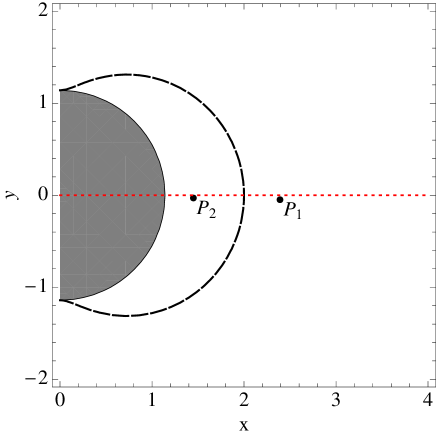
Figure 2: Graphical representation of the initial conditions, in units with $GM/c^{2}=1$. The area inside the horizon is covered in grey, the dotted red line marks the equatorial plane and the dashed black curve is the boundary of the ergoregion. $P_{1}$ corresponds to $r=r_{h}+1.25$ and $P_{2}$ to $r=r_{\rm ISCO}$. At both points, $\theta=\pi/2+0.02$, and we choose $\dot{r}=\dot{\theta}=0$. The specific angular momentum is $a=0.99$ and, therefore, $P_{2}$ lies within the ergoregion ($r_{\rm ISCO}<r_{e}$).

The explicit form of the effective potential (35) is too complicated to be illuminating, unlike the flat background case. A given orbit is determined once $j_{s}$, $j_{t}$, and initial conditions are specified. The initial conditions determine the values of the energy $E$ and angular momentum $L$, and the subsequent motion is confined to the region contained in the contour (36). The equations of motion can be integrated numerically to explore the detailed behavior of the string motion.

We will present here only results for the string motion around a rapidly spinning black hole, with $a=0.99$. This is complementary to the $a=0$ case presented by Larsen Larsen:1993nt . The role of the black hole spin is addressed below in subsection V.2.5. We consider just two sets of initial conditions for several different values of $J^{2}$ and $\omega$, which appear to be adequate for understanding the features of the motion. For both sets the string starts out at rest, $\dot{r}_{0}=\dot{\theta}_{0}=0$. The initial polar angle is fixed in both cases at $\theta_{0}=\pi/2+0.02$, just below the equatorial plane. The two cases differ only in the initial value of $r$. The two values we will explore are (somewhat arbitrarily) $r_{0}=r_{h}+1.25M\approx 2.39\,M$ and $r_{0}=r_{\rm ISCO}\approx 1.45\,M$, where $r_{\rm ISCO}$ is the radius of the innermost stable co-rotating circular orbit (ISCO) which is given in terms of $M$ and $a$ in, e.g., Ref. Bardeen:1972fi .

In Fig. 2 the two sets initial conditions correspond to points $P_{1}$ and $P_{2}$ respectively. Each point in this figure other than those on the $y$ axis corresponds to a circular ring in space. The coordinates $x$ and $y$, used as labels in this and later graphs of the $(r,\theta)$ plane, are defined by

$$x=r\sin\theta,$$ (48)

$$y=r\cos\theta.$$ (49)

The grey area indicates the region inside the horizon, the dotted red line marks the equatorial plane and the dashed black curve is the boundary of the ergoregion. For $\omega$ we consider only the three values $\omega=0,\pm 1$, since these span the full dynamical range and can be expected to frame the full picture. Note that changing the sign of $\omega$ is equivalent to changing the sign of $a$, since $\omega$ appears always multiplied by $a$ (via $g_{t\phi}$) in the equations of motion, and all other occurrences of $a$ are via $a^{2}$. Positive $\omega$ corresponds to co-rotation, while negative $\omega$ corresponds to counter-rotation.

V.2.2 Boundaries of motion

By studying the boundaries of the motion we can classify the types of dynamics and determine how they depend on the current, energy, and initial conditions. These boundaries are determined by eq. (36). For a given initial condition and current, a particular boundary is determined. These boundaries are the relativistic version of the contours plotted in Fig. 1 for a Newtonian elastic spinning ring and, as we will see shortly, the share many qualitative characteristics with their Newtonian counterparts. At the end of this subsection we give examples of such boundaries, but first we present some graphs, deduced from the potential, that allow one to see which ranges of current or energy will correspond to different qualitative types of boundaries.

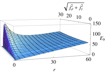
(a) $\leavevmode\nobreak\ \omega=1$

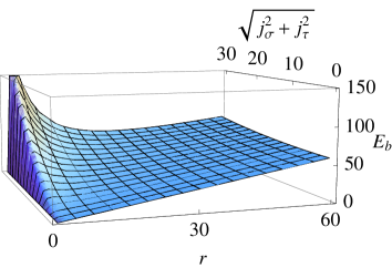
(b) $\leavevmode\nobreak\ \omega=0$

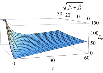
(c) $\leavevmode\nobreak\ \omega=-1$

Figure 3: Plots of the energy of a string at rest (or energy at the boundary of motion) as a function of $r$ (plots starting at $r=r_{h}$) and $\sqrt{j_{\sigma}^{2}+j_{\tau}^{2}}$, for three values of the ratio between the components of the current $\omega=-j_{\sigma}/j_{\tau}$ and at $\theta=\pi/2+0.02$ ($GM=c=\mu=1$). All graphs possess minima, which implies that bound motion is possible for energies greater than $E_{b}^{\min}$, the energy associated with the minimum. However, only for $\omega=0,-1$ is there a maximum located outside the horizon.

(a)  $r=r_{h}+1.25$, $\omega=1$

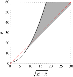
(b)  $r=r_{h}+1.25$, $\omega=0$

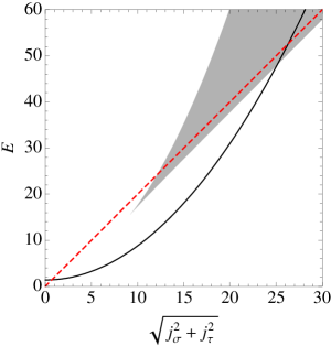
(c)  $r=r_{h}+1.25$, $\omega=-1$

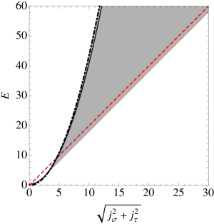
(d)  $r=r_{\rm ISCO}$, $\omega=1$

(e)  $r=r_{\rm ISCO}$, $\omega=0$

(f)  $r=r_{\rm ISCO}$, $\omega=-1$

Figure 4: Plots of the energy of a string at rest (or at the boundary of motion) as a function of $J=\sqrt{j_{\sigma}^{2}+j_{t}^{2}}$ for specific values of $\omega$ and $r$ as indicated, and for $\theta=\pi/2+0.02$ ($GM=c=\mu=1$). The solid black curve, which can be thought of as a constant $r$ slice of the graphs in Fig. 3, is the energy of the string at rest at the given radius $r$, and is the only curve on the graph that depends on the value of $r$. The dashed red line corresponds to the energy of a string at rest at infinity (the escape energy). The shaded region is the area between the curves corresponding to the minimum and the maximum of $E_{b}$ for each $J$ (cf. Fig. 3), with the exception of the $\omega=1$ cases where the dotted-dashed black curve corresponds to the value of $E_{b}$ at the horizon. These graphs allow one to infer the properties of the motion. For a given energy or value of $J$, there is a corresponding point on the solid black curve. If this point lies outside the shaded area and above the dashed red line then the motion has just an outer boundary in the $x$ direction, but the string has enough energy to potentially escape (there is no boundary in the $y$ direction). If the point lies outside the shaded area and below the dashed red line then the motion is bounded in all directions. If instead the point lies within the shaded region, then the motion has boundaries both at low and high values of $x$. Additionally, if the point lies above the dashed red line then there is no boundary on the $y$ motion and the string can potentially escape. If the point lies below the dashed red line then the motion can be trapped in some toroidal volume. Notice that for $\omega=-1$ and inside the ergosphere, Fig. 4(f), there can never be an inner boundary.

To begin with, in Fig. 3 we have plotted $E_{b}$ as a function of $J=\sqrt{j_{\sigma}^{2}+j_{\tau}^{2}}$ and $r$ for fixed $\theta=\pi/2+0.02$, which corresponds to our initial conditions, and for three different values of $\omega$. In this and all subsequent plots we adopt units with $GM=c=\mu=1$. That is, in terms of the gravitational radius $r_{g}=GM/c^{2}$, what is plotted is $E_{b}/\mu r_{g}$ and $J\sqrt{c/\mu}/r_{g}$ vs. $r/r_{g}$.

In the cases $\omega=0,-1$, where there is a maximum outside the horizon for any given value of $J$, the motion has an outer boundary in $r$ but no inner boundary if either $E<E_{b}^{\rm min}$ or $E>E_{b}^{\rm max}$, where $E_{b}^{\rm min}$ and $E_{b}^{\rm max}$ correspond to the minimum and the maximum of $E_{b}$ respectively. If $E_{b}^{\rm max}>E>E_{b}^{\rm min}$ then there will be three solutions to eq. (36), corresponding to an inner and an outer boundary and yet another outer boundary at low values of $r$. In the co-rotating case $\omega=1$, where there is no maximum, the role of $E_{b}^{\rm max}$ is played by $E_{b}^{h}$, the value of $E_{b}$ at $r=r_{h}$. For both an inner and an outer boundary to exist, the energy must fall in the range $E_{b}^{h}>E>E_{b}^{\rm min}$. Notice that in this case no string can exist outside the horizon with energy $E<E_{b}^{\rm min}$.

So far we have been discussing bounds in the radial direction near the equatorial plane. There is also a boundary in the motion along the axis if the total energy of the string is less than the energy of a string at rest at infinity, since the string must have at least this much energy in order to be able to escape. We call this energy $E_{\rm esc}$. To determine how it depends on $J$, we can use the flat background example of section V.1. Eqn. (43) gives $E_{b}=\mu\rho+J^{2}/\rho$, whose minimum lies at $E_{\rm esc}(J)=2J\sqrt{\mu}$.

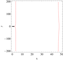
(a)  $E=50$, $\omega=1$

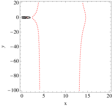
(b)  $E=17$, $\omega=1$

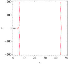
(c)  $E=50$, $\omega=0$

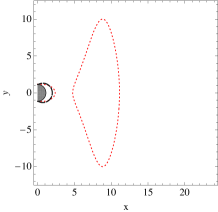
(d)  $E=17$, $\omega=0$

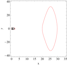
(e)  $E=50$, $\omega=-1$

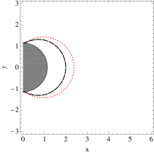
(f)  $E=17$, $\omega=-1$

Figure 5: Boundaries of motion for different values of the energy and the $\omega$ parameter, for string starting at rest at $r=r_{h}+1.25$ and $\theta=\pi/2+0.02$. The grey area represent the region inside the event horizon, the dashed black curve the boundary of the ergoregion and the dashed red line the boundaries of motion. The form of the boundaries is exactly what one could have predicted by using Figs. 4(a)-4(c).

Fig. 4 presents plots that allow one to see how the qualitative properties of the motion depend on $J$, for specific values of $\omega$ and the initial $r$ as indicated, and for $\theta=\pi/2+0.02$. The solid black curve, which can be thought of as constant $r$ slice of the graphs in Fig. 3, is the energy (36) of the string at rest at the given radius $r$, and is the only curve on the graph which depends on the value of the initial $r$. The dependence on $\omega$ comes in only through the $g_{t\phi}$ term in (36). Increasing $\omega$ acts to raise the energy for a given $J$. The dashed red line corresponds to the energy of a string at rest at infinity (the escape energy). The shaded region is the area between the curves corresponding to the minimum and the maximum of $E_{b}$ for each $J$ (cf. Fig. 3), with the exception of the $\omega=1$ cases where the dotted-dashed black curve corresponds to the value of $E_{b}$ at the horizon.

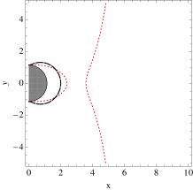
(a)  $E=50$, $\omega=0$

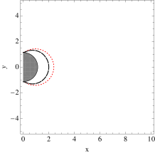
(b)  $E=50$, $\omega=-1$

Figure 6: Magnified segments of Fig. 5(c) and 5(e) which demonstrate the existence of yet a third boundary of motion for $\omega=0,-1$. This acts as a second outer boundary, therefore forbidding any string starting from inside the region bounded by the innermost red dotted curve to ever leave this region.

We now demonstrate how one can infer all the qualitative information about the boundaries of the motion from Fig. 4. For a given energy or value of $J$, there is a corresponding point on the solid black curve. This point can lie in several distinct regions of the graph, which correspond to qualitatively different types of boundary:

1. A region outside the shaded area and above the dashed red line. In this case there is just an outer boundary, i.e. there is only one value of $r$ outside the horizon that yields a solution to eq. (36) for each $\theta$ for given $E$ and $J$. The string can potentially escape in the $y$ direction, as its energy is higher than the $E_{\rm esc}$.

2. A region outside the shaded area and below the dashed red line. Again, there is just an outer boundary. However, now the string cannot escape in the $y$ direction as its energy is lower than the $E_{\rm esc}$.

3. A region inside the shaded area and above the dashed red line. In this case there are always outer and inner boundaries, and for the examples with $\omega=0,-1$ there is yet another outer boundary at a lower value of $x$. That is, eq. (36) has up to three solutions for $r$ outside the horizon each value of $\theta$ and for given $E$ and $J$. However, there is no boundary on the $y$ motion and the string can potentially escape.

4. A region inside the shaded area and below the dashed red line. The boundaries of the motion are the same in number as in the previous case, but with a qualitative difference: the inner and the outer boundaries at higher values of $x$ meet at a certain value of $y$ and together form a closed curve. Therefore, there is also effectively a boundary in the $y$ motion and the string can be trapped in some toroidal volume.

There is a subtle point that should not pass unnoticed: depending on the initial conditions, a string with given $E$ and $J$ which corresponds to a point in the shaded region in Fig. 4 can either be moving in between the inner and outer boundary at higher $x$’s, or it can be inside the second outer boundary at smaller $x$’s. Finally it should be stressed that a second outer boundary at small $x$’s can only exist when there $E_{b}$ has a maximum outside the horizon.

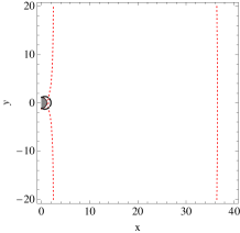
(a)  $E=38$, $\omega=1$

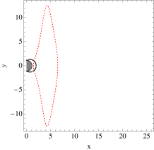
(b)  $E=8$, $\omega=1$

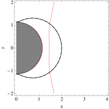
(c)  $E=38$, $\omega=1$

(d)  $E=8$, $\omega=1$

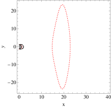
(e)  $E=38$, $\omega=0$

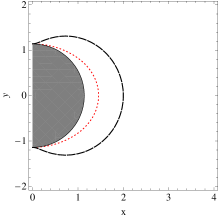
(f)  $E=8$, $\omega=0$

Figure 7: Boundaries of motion for different values of the energy and the $\omega$ parameter, for string starting at rest at $r=r_{\rm ISCO}$ and $\theta=\pi/2+0.02$. The form of the boundaries is exactly what one could have predicted by using Figs. 4(d)-4(f). Figs. 7(c) and 7(d) focus on the region close to the black hole of Figs. 7(a) and 7(b) respectively. Clearly, the inner boundary of motion lies within the ergoregion.

Next we give in Fig. 5 a few examples of plots of the boundaries of motion corresponding to given initial conditions and current (or energy), for $r=r_{h}+1.25$. The qualitative nature of these boundary plots can be read off from Fig. 4. For example, with $E=50$ there exist both inner and outer boundaries in the $x$ direction for all values of $\omega$, corresponding to the fact that the solid black curve in Figs. 4(a), 4(b), 4(c) falls inside the shaded region when $E=50$. Additionally, for $\omega=1,0$ there is no boundary along the $y$ direction, whereas for $\omega=-1$ there is such a boundary, corresponding to the fact that in the latter case the $E=50$ point on the solid black curve lies below the dashed red line in Fig. 4(c). In Fig. 6, one can see the region closer to the black hole: for the $\omega=0,-1$ cases, there exists a third boundary, which is an outer boundary. This is in accordance with the form of $E_{b}$ in Figs. 3(b) and 3(c) and highlights the subtlety discussed above right after outlining the various regions of Fig. 4. For $E=17$ on the other hand, only the $\omega=1$ choice allows motion which is unbounded in the $y$ direction. For $\omega=0$ the string is trapped in a toroidal volume, and for $\omega=-1$ there is only an outer boundary. Fig. 7 is similar to Fig. 5, but for $r=r_{\rm ISCO}$. (We do not plot the $\omega=-1$ case since there is no energy for which there will be an internal boundary for the motion.) In this case, the inner boundary of motion lies within the ergoregion.

Before closing this section it is worth stressing once more the similarity between the contour plots of the boundaries of motion for a Newtonian elastic spinning ring presented in Fig. 1 and the boundaries of motion for the relativistic strings presented in this section.

V.2.3 Trajectories

In this subsection we look at examples of individual trajectories, and in particular we exhibit processes whereby a string is ejected along the axis, with some of the initial internal energy of the string converted to translational kinetic energy. To this end, we employed numerical integration with Mathematica 6.0 to solve the equations of motion. As already mentioned we consider here two different initial conditions: one for which the string starts outside the ergoregion, and one for which the string starts at $r=r_{\rm ISCO}$, which lies well within the ergoregion (points $P_{1}$ and $P_{2}$ in Fig. 2 respectively). Starting at rest from these initial positions, there are three types of trajectories, as indicted by the types of boundaries of motion: those that are trapped inside an outer boundary with no inner boundary and simply fall in across the horizon, those that are trapped in some toroidal volume, and those that can reach spatial infinity along the direction of the axis. The trajectories of the first type display no interesting features so we do not present any explicit examples of them here.

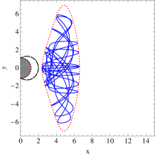
(a)  $E=9$, $r=r_{h}+1.25$

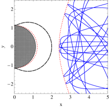
(b)  $E=9$, $r=r_{h}+1.25$

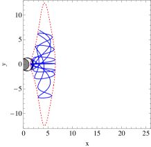
(c)  $E=8$, $r=r_{\rm ISCO}$

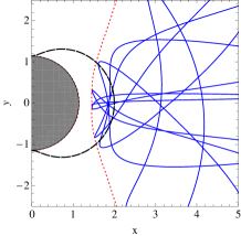
(d)  $E=8$, $r=r_{\rm ISCO}$

Figure 8: Confined trajectories of the string for different initial positions and different energies. The blue continuous line corresponds to the trajectory of a point on the string ($\phi$ dimension suppressed). No qualitative difference seems to exist between the motion of a string starting inside the ergoregion and one starting outside. In both case the motion seems to follow no clear pattern.

We begin by discussing bound trajectories. The energies we considered previously do not lead to confined motion for a string starting at $P_{1}$. This can be seen in Fig. 5: For the cases where there can be confined motion, namely Figs. 5(d) and 5(e), our initial position lies on the innermost outer boundary. Thus the string would fall straight into the black hole. However, for other energies there can be confined motion for a string starting at $P_{1}$. Also, according to Fig. 7(b) we have already found an example where the string’s motion is confined when it starts from $P_{2}$, i.e. inside the ergoregion. In Fig. 8 we present the motion of a string starting from $P_{1}$ with $E=9$ and that of a string starting from $P_{2}$ with $E=8$ for qualitative comparison. Both cases refer to $\omega=1$ (co-rotation). In both cases the strings move somewhat randomly, without following any clear pattern. Fig. 8(b) and 8(d) focus on the area inside and around the ergoregion. The string is sometimes pulled by gravity rather sharply back toward the equatorial plane after reflecting from the inner boundary. We have monitored the accuracy by running the code backward in time from the point the forward run ended, and checking how closely this backward run approaches the initial conditions. In the plots presented we stop the simulation before the accuracy becomes lower than $10^{-4}$.

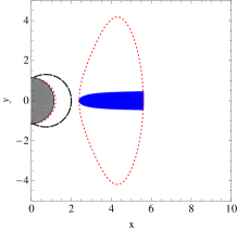
(a)  $E=8$, $r=r_{h}+1.25$

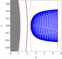
(b)  $E=8$, $r=r_{h}+1.25$

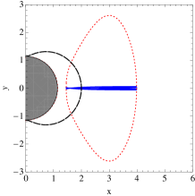
(c)  $E=5.5$, $r=r_{\rm ISCO}$

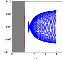
(d)  $E=5.5$, $r=r_{\rm ISCO}$

Figure 9: “Focusing” of the trajectories. In this case a pattern seems to be arising. In Figs. 9(b) and 9(d) we have distorted the aspect ratio in order to make this manifest.

Before proceeding further to trajectories that can reach spatial infinity, there is another interesting feature of confined motion which should not be missed. In Fig. 9 we present confined trajectories starting from $P_{1}$ with $E=8$ and from $P_{2}$ with $E=5.5$, always for $\omega=1$. There is evidently some remarkable “focusing” of the motion close to the equatorial plane in both cases, and a very regular pattern is generated. In Figs. 9(b) and 9(d) we have distorted the aspect ratio in order to make manifest the pattern that arises in the motion. We do not understand why these cases are so different from those shown in Fig. 8. The focussing cannot be explained by considering only the boundary of allowed motion (dotted curve) as inferred using the effective potential. The appearance of a Lissajous-like pattern indicates that when the string stays close to the equatorial plane the motion becomes similar to complex periodic oscillation.

Finally, we discuss trajectories that can reach spatial infinity. In Fig. 10(a) we have plotted the trajectory of a string starting from $P_{1}$ with $E=17$ and $\omega=1$. After a couple of oscillations around the equatorial plane, which are exhibited more clearly in Fig. 10(b), the string escapes along the $z$ direction. The behavior of a string starting from $P_{2}$ with $E=38$ and $\omega=1$ is quite similar. In both cases, there is some conversion of internal energy of the string into kinetic energy along the $y$ axis.

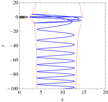
(a)  $E=17$, $r=r_{h}+1.25$

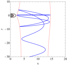
(b)  $E=17$, $r=r_{h}+1.25$

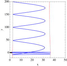
(c)  $E=38$, $r=r_{\rm ISCO}$

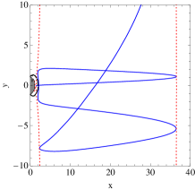
(d)  $E=38$, $r=r_{\rm ISCO}$

Figure 10: Escape trajectories for strings of different energy and angular momentum, start at $P_{1}$ and $P_{2}$ respectively. After some oscilations around the equatorial plane the strings escape to infinity along the axis of symmetry. Clearly there is some conversion of internal to kinetic energy.

Another interesting class of non-confined trajectories are the scattering trajectories found by Larsen in Ref. Larsen:1993nt . An example of such a trajectory for a string with $E=11.2929$, $\omega=1$, and initial conditions $r_{0}=200$, $\theta_{0}=3.11$, $\dot{r}_{0}=-3.4$ and $\dot{\theta}_{0}=-0.007$ is shown in Fig. 11(a). The string comes in along the axis and after a couple of bounces around the black hole, which can be better appreciated in Fig. 11(b), escapes to infinity out the other side. The scattering in this case reduces the mean radius in the $x$ direction, signaling a conversion of internal energy to kinetic energy along the $y$ direction, as explained below in the next subsection, V.2.4.

In Figs. 11(c) and 11(d) we show a case where the string actually falls into the black hole instead if getting scattered. For this case, $E=11.8417$, $\omega=1$, and the initial conditions are $r_{0}=200$, $\theta_{0}=3.11$, $\dot{r}_{0}=-2.4$ and $\dot{\theta}_{0}=-0.007$. In this case the string has more energy than a string at rest on the horizon and, hence, its motion has no inner boundary close to the equatorial plane (cf. the discussion in section V.2.2 about Figs. 3(a) and 4).

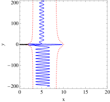
(a)  $E=11.3$, scattering

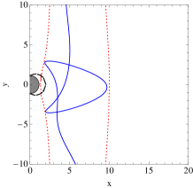
(b)  $E=11.3$, scattering

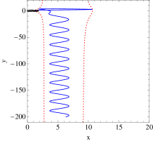
(c)  $E=11.8$, collapse

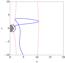
(d)  $E=11.8$, collapse

Figure 11: Scattering and collapse on the black hole of strings coming from spatial infinity. The scattering can lead to energy conversion, as can be seen from Fig. 11(a) by the fact that the average radius of oscillation along the $x$ direction has been slightly reduced after the scattering. On the other hand, if the inner boundary of motion lies within the horizon close to the equatorial plane, then instead of a scattering there can be a collapse, see Figs. 11(c) and 11(d).

V.2.4 Ejection energy

As noted, on some trajectories internal energy of the string can be converted to translational kinetic energy along the axis. To characterize this energy we may associate a relativistic boost factor $\Gamma=E/E_{0}$ with the asymptotic string, where $E_{0}$ is the energy of the string in its center of mass frame at infinity. In the center of mass frame, all velocities vanish at the inner and outer boundaries $\rho=\rho_{i,o}$ of oscillation, so we may use (43) to obtain $E_{0}=\rho+J^{2}/\rho$. Eliminating $J$ we find $E_{0}=\rho_{i}+\rho_{o}$. Thus, using the present notation $x$ for the cylindrical radius, we have

$$\Gamma=\frac{E}{x_{i}+x_{o}}.$$ (50)

With this relation the $\Gamma$ factors corresponding to the processes shown in the previous examples can be computed. For example, for the $E=17$ case in Fig. 10 we find $\Gamma\approx 1.01$, or $v/c\approx 0.15$, and for the $E=38$ case we find $\Gamma\approx 1.09$, or $v/c\approx 0.39$. We expect that these mildly relativistic boost factors are typical of what one can expect in generic cases.

V.2.5 The role of black hole spin

The black hole spin enters the string dynamics via the $a$ dependence of the various metric coefficients. While the value of $a$, certainly affects the boundaries of motion and dynamics when other quantities are held fixed, we do not see any systematic qualitative effect that can be attributed uniquely to the spin. That is, by varying the current, energy, and location of the string similar effects can be produced. This statement is based both on examining cases (not explicitly reported here) for which $a=0$, as well as by comparing the behaviors for different values of $\omega$. The dynamics only depends on $\omega$ when $a$ is non-zero, but the effect of changing $\omega$ can also generally be reproduced by changing other quantities.

The one exception to this statement concerns the issue of negative Killing energy states. In the presence of black hole spin, there is an ergoregion, inside of which such states exist for point particles. The same is true for the string, though the mechanism is a bit different.

For a particle, negative angular momentum orbits in the ergoregion have negative Killing energy. Longitudinal motion of a string is meaningless, so it is not the “orbital” motion, but rather the current on the worldsheet that can access negative energy states. In particular, the second term on the right hand side of the energy (36), i.e. $-g_{t\phi}\tilde{\Sigma}^{\sigma\tau}=|g_{t\phi}/g_{\phi\phi}|L/2\pi$, is negative there when the angular momentum $L=4\pi\omega J^{2}/(1+\omega^{2})$ is negative. The first term in eq. (36) vanishes at the horizon, so the energy is certainly negative there when $L<0$. The negative energy states extend out a certain distance (which depends on the values of $\omega$ and $J$) from the horizon into the ergoregion. For example, one can see in Fig. 4(f) the negative energy states at $r_{\rm ISCO}$ in the case $\omega=-1$, except for the smallest values of $J$. (For the limiting case of zero tension and $\omega=-1$, there are negative energy states everywhere in the ergoregion.)

VI Relevance to Astrophysics?

As stated in the Introduction, although our primary aim in this paper was to study the motion of a current carrying strings in a Kerr background as an interesting dynamical system, our investigation was also loosely motivated by the problem of the production of collimated jets in astrophysics. We should therefore like to comment on what might be the relevance of our findings to astrophysical systems.

First of all, the current carried by the string in the model need not represent an electric current, but it can just serve to model the role of angular momentum. In this sense, a current carrying string can serve as an idealization of some MHD matter configuration with tension and angular momentum, as mentioned in the Introduction. Simplistic as it may be, this allows for the identification of a mechanism that might conceivably be relevant: the tension sets a barrier for the motion that keeps the string within a certain radius from the axis of symmetry, while the angular momentum sets a barrier that keeps the string outside a certain radius. Gravity deforms these barriers creating either a closed region in which the string is trapped, or a “restricted path” that leads to motion along the symmetry axis. If some physical process were to “feed” such a system with strings close to the equatorial plane, then under the right circumstances one might end up with a very well collimated stream of strings moving out along the axis of symmetry. Of course, the axisymmetry we are imposing might be too restrictive, and in particular, even if a string started out approximately axisymmetric, it might wobble or twist and reconnect. Perhaps the tension could act to suppress such effects, but this requires further investigation.

Still, one may speculate that the general flavor of the mechanism exhibited by the strings might generically be present in a class of astrophysical systems. For instance, given a system with an accretion disk, plasma leaving the inner edge of the disk would carry some angular momentum, and plasma flux tubes do possess a significant tension (which however is not constant but grows in proportion to the length). It might even be that differential rotation can stretch such a tube, storing in it a large amount of electromagnetic energy before launching it towards the axis. External magnetic fields, which have been left out of consideration in our initial study, might also play an important role in the subsequent dynamics. It remains to be seen whether aspects of this picture could actually be astrophysically relevant.

Regarding the energetics, it should be noted that the mechanism described here does not lead to significant (ultra-relativistic) acceleration of the strings. While internal energy of the string can be converted to kinetic energy of motion along the axis of symmetry, the resulting $\Gamma$ factors in the examples we studied are rather close to unity, the largest velocity we reported being $0.39c$. Therefore, even if the mechanism we have found is somehow relevant to collimation, it does not appear able to explain the acceleration of relativistic jets. The acceleration would have to occur due to the presence of electromagnetic fields, or to some other mechanism. In particular, the process discussed here does not tap into the rotational energy of the black hole, which is a prime candidate for the source of ultra-relativistic jet energy.

On the contrary, the collimation effect we find persists even at the Newtonian level, which may be advantageous: collimated jets seem to be present not only around black holes, but also around objects with significantly weaker gravitational fields, such as accreting young stars for instance livio . Therefore, if there is a common mechanism for the collimation, it should not depend on relativistic effects. Hence, the effects described here could perhaps be part of a more involved process that collimates and drives astrophysical jets.

VII Conclusions

We have studied the motion of relativistic, current carrying strings moving axisymmetrically on the background of a Kerr black hole. First the equations of motion and conserved quantities in the conformal gauge were found. Next, we determined how the energy of a string that is instantaneously at rest depends on the current and the position of the string. Contours of this quantity determine boundaries of the possible motion of a string with that energy and current. We compared this analysis with that for a Newtonian elastic ring moving around a point mass, and found that system to be qualitatively similar.

By considering a number of examples and various plots of the relevant functions, the possible types of motion were mapped out. Regions of parameters for which the string falls into the black hole, or is trapped in a toroidal volume, or can escape to infinity, were identified. After this general analysis, we examined representative trajectories found by numerical integration, illustrating various interesting behaviors. In particular, we found that a string can start out at rest near the equatorial plane and, after bouncing around, be ejected out along the axis, some of its internal (elastic or rotational kinetic) energy having been transformed into translational kinetic energy. The resulting velocity can be an order unity fraction of the speed of light.

Finally, we addressed the question of possible astrophysical significance of this system as a simple model of MHD plasma flux tubes, which might conceivably play a role in jet formation and collimation.

- (1) A. L. Larsen, “Chaotic string capture by black hole,” Class. Quant. Grav. 11, 1201 (1994) [arXiv:hep-th/9309086].
- (2) A. V. Frolov and A. L. Larsen, “Chaotic scattering and capture of strings by a black hole,” Class. Quant. Grav. 16, 3717 (1999) [arXiv:gr-qc/9908039].
- (3) M. Livio, “Astrophysical jets: a phenomenological examination of acceleration and collimation,” Phys. Rep. 311, 225 (1999).
- (4) M. Christensson and M. Hindmarsh, “Magnetic fields in the early universe in the string approach to MHD,” Phys. Rev. D 60, 063001 (1999) [arXiv:astro-ph/9904358].
- (5) V. S. Semenov, S. A. Dyadechkin, I. B. Ivanov and H. K. Biernat, “Energy confinement for a relativistic magnetic flux tube in the ergosphere of a Kerr black hole,” Phys. Scripta 65, 13 (2002).
- (6) V. Semenov, S. Dyadechkin and B. Punsly, Science 305, 978 (2004) [arXiv:astro-ph/0408371].
- (7) H. C. Spruit, “Equations for thin flux tubes in ideal MHD,” Astron. Astrophys. 102, 129 (1981).
- (8) A. L. Larsen, “Dynamics of cosmic strings and springs: A Covariant formulation,” Class. Quant. Grav. 10, 1541 (1993) [arXiv:hep-th/9304086].
- (9) A. Villenkin and E. P. S. Shellard, Cosmic Strings and Other Topological Defects, (Cambridge University Press, Cambridge, 1994).
- (10) M. B. Hindmarsh and T. W. B. Kibble, “Cosmic strings,” Rept. Prog. Phys. 58, 477 (1995) [arXiv:hep-ph/9411342].
- (11) B. Carter, P. Peter and A. Gangui, “Avoidance of collapse by circular current-carrying cosmic string loops,” Phys. Rev. D 55, 4647 (1997) [arXiv:hep-ph/9609401].
- (12) B. Carter, “Brane dynamics for treatment of cosmic strings and vortons,” arXiv:hep-th/9705172.
- (13) A. L. Larsen, “Charged circular test string in external magnetic fields,” Mod. Phys. Lett. A 7, 2913 (1992).
- (14) A. L. Larsen, “Charge current carrying circular strings in arbitrary backgrounds,” Phys. Lett. A 170, 174 (1992).
- (15) S. A. Dyadechkin, V. S. Semenov, H. K. Biernat and T. Penz, “Comparison Of Magnetic Flux Tube And Cosmic String Behavior In Kerr Metric,” Adv. Space Res. 42, 565 (2008).
- (16) F. Dubath, M. Sakellariadou and C. M. Viallet, “Scattering of cosmic strings by black holes: Loop formation,” Int. J. Mod. Phys. D 16, 1311 (2007) [arXiv:gr-qc/0609089].
- (17) M. Snajdr and V. P. Frolov, “Capture and critical scattering of a long cosmic string by a rotating black hole,” Class. Quant. Grav. 20, 1303 (2003) [arXiv:gr-qc/0211018].
- (18) M. Snajdr, V. P. Frolov and J. P. DeVilliers, “Scattering of a long cosmic string by a rotating black hole,” Class. Quant. Grav. 19, 5987 (2002) [arXiv:gr-qc/0208009].
- (19) E. Witten, “Superconducting Strings,” Nucl. Phys. B 249, 557 (1985).
- (20) J. M. Bardeen, W. H. Press and S. A. Teukolsky, “Rotating Black Holes: Locally Nonrotating Frames, Energy Extraction, And Scalar Synchrotron Radiation,” Astrophys. J. 178, 347 (1972).