CERN-PH-TH/2008-249

MCTP-08-67

Vacuum Stability with Tachyonic Boundary
Higgs Masses in No-Scale Supersymmetry
or Gaugino Mediation

Jason L. Evans^a,b, David E. Morrissey^c, James D. Wells^a,b

^a Michigan Center for Theoretical Physics (MCTP)
University of Michigan, Ann Arbor, MI 48109
^b CERN, Theory Division, CH-1211 Geneva 23, Switzerland
^c Jefferson Laboratory of Physics, Harvard University
Cambridge, Massachusetts 02138

No-scale supersymmetry or gaugino mediation augmented with large negative Higgs soft masses at the input scale provides a simple solution to the supersymmetric flavor problem while giving rise to a neutralino LSP. However, to obtain a neutralino LSP it is often necessary to have tachyonic input Higgs soft masses that can give rise to charge-and-color-breaking (CCB) minima and unbounded-from-below (UFB) directions in the low energy theory. We investigate the vacuum structure in these theories to determine when such problematic features are present. When the standard electroweak vacuum is only metastable, we compute its lifetime under vacuum tunneling. We find that vacuum metastability leads to severe restrictions on the parameter space for larger $\tan\beta\sim 30$, while for smaller $\tan\beta\sim 10$, only minor restrictions are found. Along the way, we derive an exact bounce solution for tunneling through an inverted parabolic potential.

1 Introduction

Supersymmetry (SUSY) is a well-motivated extension of the Standard Model (SM) that provides an explanation for the stability of the hierarchy between the weak scale and the Planck scale [1]. However, experiment excludes SUSY from being an exact symmetry at low energies. If supersymmetry is softly broken, it is possible to push the superpartner masses up enough to make the theory consistent with experiment while still preserving the electroweak-gravity hierarchy. For this to work, the masses of the SM superpartners should not be significantly larger than the electroweak scale, putting them within reach of upcoming particle collider experiments such as the LHC.

A major drawback of this scenario of softly-broken low-energy supersymmetry is that the supersymmetry breaking operators generically introduce many new sources of quark and lepton flavor mixing, leading to flavor-changing neutral currents (FCNC) in conflict with experiment [2]. One way to cure this problem is to take No-Scale boundary conditions in which the soft scalar masses and couplings all vanish at a boundary input scale, with the gaugino soft masses being the only significant source of supersymmetry breaking in the visible sector at this scale [3]. Such boundary conditions can arise from gaugino mediation [4], or conformal running effects [5, 6, 7, 8, 9]. Low-scale scalar soft terms, which are necessary to obtain a viable phenomenology, are generated primarily from the gaugino masses in the course of renormalization group (RG) running from the boundary input scale down to near the electroweak scale. This dominant contribution is controlled by gauge interactions, implying that the regenerated scalar soft terms, and thus the squark and slepton masses, will be approximately flavor-universal at the low scale.

A slight generalization of this pure No-Scale picture, which still leads to scalar soft terms that are roughly flavor universal at the low scale (for the first and second generations), is to allow non-vanishing Higgs soft scalar masses at the boundary scale. In the context of gaugino mediation this can arise if the Higgs multiplets propagate in the bulk [5], while for conformal running, it can emerge from hidden-sector interactions related to the origin of the $\mu$ term [8, 9, 10]. These Higgs Exempt No-Scale (HENS) models often have an important phenomenological advantage over pure No-Scale constructions: in large regions of the parameter space HENS models have a neutralino lightest superpartner particle (LSP) [11]. This differs from the situation in strict No-Scale models where typically the predominantly right-handed stau is the lightest SM superpartner particle [12]. While such models can be viable if the true LSP is a gravitino [13], a neutralino LSP with exactly conserved $R$-parity tends to make for a better thermal dark matter candidate.

HENS models can push the right-handed stau mass above that of the lightest neutralino by the influence of the non-vanishing Higgs soft masses on the RG running of the other soft parameters. The primary contribution to the slepton soft terms comes from the hypercharge $D$ term $S_{Y}=Tr(Y\,m^{2})\simeq(m_{H_{u}}^{2}\!-\!m_{H_{d}}^{2})/2$ that appears in the RG equations for all the MSSM scalar soft masses [14, 15, 12]. This contribution increases the right-handed slepton soft masses in the course of running down provided $S_{Y}$ is negative. In the portion of the HENS model parameter space that is also consistent with electroweak symmetry breaking, the Higgs scalar soft masses must typically be very tachyonic at the boundary scale to obtain a neutralino LSP, and the uncolored sfermions still end up being relatively light [11].

While these HENS models are compelling, the tachyonic Higgs soft masses at the boundary scale lead to concerningly large tachyonic low-scale Higgs soft masses. These, combined with the small (but positive) slepton soft masses, suggest that the true vacuum of the theory might be a charge-and-color-breaking (CCB) minimum, or there may exist unbounded-from-below (UFB) directions that are only stabilized far out in field space by higher-dimensional operators [16, 17, 18, 19, 20, 21]. The presence of such features need not exclude these regions of the parameter space provided our SM electroweak vacuum is metastable and long-lived relative to the age of the universe.

In the present work we study the vacuum structure of HENS models, and compute the lifetime of the SM vacuum state when it turns out to be metastable. We concentrate on the stability of the SM vacuum at zero temperature with respect to vacuum tunneling. Thermal effects in the early universe can also potentially induce thermal transitions between different vacua, and modify the shape of the potential itself. However, these thermal effects tend to stabilize the origin of the field space to which the SM vacuum is connected, favoring this vacuum over others that lie further out in the field space [22]. Thermal effects are especially effective in delaying the formation of vacua that break color due to the large thermal corrections from the strong gauge and top quark Yukawa couplings [22, 20, 23]. Scalar field evolution during and after inflation may also populate non-standard vacua, although the precise result depends on the details of inflation and lies beyond the scope of this paper [24, 21]. By focusing solely on the $T=0$ constraints we obtain conservative and unambiguous bounds on the HENS parameter space that do not depend on the cosmological history.

Motivated by gauge coupling unification, throughout this work we take the input scale to be $M_{c}=10^{16}\,\,{\rm GeV}$ and we assume a universal gaugino mass $m_{1/2}$ at this scale. The set of independent free parameters after imposing consistent electroweak symmetry breaking is therefore

$$m_{1/2},~{}~{}~{}\tan\beta,~{}~{}~{}m_{H_{u}}^{2}(M_{c}),~{}~{}~{}m_{H_{d}}^{2}(M_{c}).$$ (1)

Investigations of No-Scale models with non-universal gaugino masses can be found in Refs. [25, 26]. Similar input soft terms have also been studied in the context of Refs. [27, 28]

The outline of this paper is as follows. In Section 2 we investigate the vacuum structure of HENS models. We discuss the general features of vacuum tunneling and outline the relevant criteria we use to judge which of the possible CCB and UFB vacua are the most dangerous in Section 3. In Section 4 we map out the portions of parameter space that are phenomenologically consistent and give rise to a SM vacuum state that is sufficiently long-lived. Section 5 is reserved for our conclusions. In Appendix A we outline our numerical technique for estimating the vacuum tunneling rate. We present in Appendix B an exact tunneling solution for an inverted-parabola barrier.

2 UFB Directions and CCB Minima in the HENS Model

With the HENS model input parameters of Eq. (1), relatively small slepton soft masses as well as large tachyonic Higgs soft masses obtain near the electroweak scale in much of the phenomenologically allowed parameter space [11]. This spectrum of soft parameters frequently implies the existence of UFB directions and CCB minima that are much deeper than the standard electroweak vacuum. Indeed, we find that nearly the entire allowed parameter space in the HENS model (before imposing vacuum stability constraints) has at least one UFB direction. We investigate the existence and nature of such potentially dangerous vacuum features in the present section.

Given the soft breaking spectrum that arises in the HENS scenario, the results of Ref. [18] suggest that the most dangerous vacuum feature will be a sleptonic UFB-3 direction. This direction has $H_{d}=0$, with $\tilde{\tau}_{L}$, $\tilde{\tau}_{R}$, $\tilde{\nu}_{L_{i\neq 3}}$, and $H_{u}^{0}$ all non-zero. Turning on expectation values for these fields, there exists a $D$- and $F$-flat direction that is only lifted by quadratic supersymmetry breaking operators. To obtain $F$-flatness, only the $F$-term of $H_{d}$ must be cancelled. This can be arranged by taking

$$|\tilde{\tau}|=|\tilde{\tau}_{L}|=|\tilde{\tau}_{R}|=\sqrt{\left|\frac{\mu}{y_{\tau}}\,H_{u}^{0}\right|},$$ (2)

with the relative phase of $\tilde{\tau}_{L}$ and $\tilde{\tau}_{R}$ chosen appropriately. $D$-flatness is then obtained by setting

$$|\tilde{\nu}_{L_{i\neq 3}}|^{2}=-\left(\frac{4\,m_{L_{i}}^{2}}{g^{2}+g^{\prime 2}}\right)+|\tilde{\tau}|^{2}+|H_{u}^{0}|^{2},$$ (3)

and represents the lowest-energy $F$-flat field configuration provided

$$|H_{u}^{0}|>\sqrt{\left|\frac{\mu}{2y_{\tau}}\right|^{2}+\frac{4m_{L_{i}}^{2}}{(g^{2}+g^{\prime 2})}}-\left|\frac{\mu}{2y_{\tau}}\right|.$$ (4)

The scalar potential along this direction in field space then becomes [18]

$$V_{UFB-3}=(m_{H_{u}}^{2}+m_{L_{i}}^{2})|H_{u}^{0}|^{2}+\left|\frac{\mu}{y_{\tau}}\right|\,(m_{L_{3}}^{2}+m_{E_{3}}^{2}+m_{L_{i}}^{2})\,|H_{u}^{0}|-\frac{2m_{L_{i}}^{4}}{g^{2}+g^{\prime 2}}.$$ (5)

When $(m_{H_{u}}^{2}+m_{L_{i}}^{2})$ is negative, the potential becomes unbounded in the limit $|H_{u}^{0}|\to\infty$. It will ultimately be stabilized by loop corrections or higher-dimensional operators (that we have not included in Eq. (5)) at a location that is very deep and far out in field space relative to the electroweak vacuum.

This sleptonic UFB-3 direction is particularly dangerous in the HENS models on account of the large and negative values of $m_{H_{u}}^{2}$ and the smaller values of $m_{L_{i}}^{2}$ and $m_{E_{i}}^{2}$ that emerge in the low-energy spectrum. These properties imply that the barrier against tunneling from the electroweak vacuum near the origin out to the deeper UFB-3 direction, arising from the linear term in $|H_{u}^{0}|$ in Eq. (5), will not be especially large. The barrier will be further weakened by larger values of $\tan\beta$ which enhance the coupling $y_{\tau}=m_{\tau}/v\cos\beta$. Other similar UFB-3 directions may be present in the theory, but they will generally have larger barriers due to the larger values of the squark soft masses or the smaller values of the first- and second-generation lepton Yukawa couplings.

When $|H_{u}^{0}|$ does not satisfy the bound given in Eq. (4), the lowest-energy $F$-flat direction in the potential has $|\tilde{\nu}_{L_{i}\neq 3}|=0$, and is given by [18]

$$V_{UFB-3}=m_{H_{u}}^{2}|H_{u}^{0}|^{2}+\left|\frac{\mu}{y_{\tau}}\right|(m_{\tilde{\tau}_{L}}^{2}+m_{\tilde{\tau}_{R}}^{2})|H_{u}^{0}|+\frac{1}{8}(g_{1}^{2}+g_{2}^{2})\,\left(|H_{u}^{0}|^{2}+\left|\frac{\mu}{y_{\tau}}\right||H_{u}^{0}|\right)^{2}.$$ (6)

This potential is no longer $D$-flat, and is stabilized at a finite value of $|H_{u}^{0}|$. If this point occurs with $|H_{u}^{0}|$ less than the bound of Eq. (4), it is a constrained local CCB minimum. On the other hand, when this constrained local extremum has $|H_{u}^{0}|$ larger than the bound of Eq. (4), it represents a saddle point that is unstable under flowing to a non-zero value of $|\tilde{\nu}_{L_{i\neq 3}}|$.

In practice, we find that for smaller values of $|H_{u}^{0}|$ the potential can be reduced further by relaxing the $F$-flatness constraint of Eq. (2). The effect of dropping the $F$-flatness constraint is that the minimal potential for a given value of $|H_{u}^{0}|$ is deformed slightly away from the precise UFB-3 form of Eqs. (5,6), but that the same qualitative features remain. In particular, there usually remains a local extremum at $|H_{u}^{0}|\neq 0$ and $|\tilde{\nu}_{L_{i\neq 3}}|=0$. We shall designate this local extremum as CCB-4. If this extremum occurs at smaller values of $|H_{u}^{0}|$, on the order of the electroweak scale, it can be a local CCB minimum. When the CCB-4 extremum occurs with a value of $|H_{u}^{0}|$ much larger than the electroweak scale, it is generally a saddle point that flows in the $\tilde{\nu}_{L_{i\neq 3}}$ direction to a genuine UFB-3 direction of the form given in Eq. (5). Even when it is only a saddle, the CCB-4 point plays an important role in determining the tunneling rate from the electroweak minimum to the UFB-3 direction, as we will discuss below.

A stable CCB-4 minimum with stops can also arise for smaller values of $\tan\beta$ and a correspondingly larger $y_{t}$ Yukawa coupling. In this case we have $H_{u}=0$ while $|\tilde{t}_{L}|=|\tilde{t}_{R}|=|\tilde{t}|$ and $H_{d}^{0}$ are all non-zero. The relevant potential is

$$V_{D}=m_{H_{d}}^{2}|H_{d}^{0}|^{2}+(m_{\tilde{t}_{L}}^{2}+m_{\tilde{t}_{R}}^{2})|\tilde{t}|^{2}+|\mu\,H_{d}-y_{t}\tilde{t}^{2}|^{2}+\frac{g^{2}+g^{\prime 2}}{8}\left(|H_{d}|^{2}+|\tilde{t}|^{2}\right)^{2}.$$ (7)

This potential is generally stable against excursions in the $|\tilde{d}|=|\tilde{d}_{L_{i\neq 3}}|=|\tilde{d}_{R_{i\neq 3}}|$ direction on account of the larger squark soft masses that arise in the HENS model. With $m_{H_{d}}^{2}<0$ at the low scale, this potential often has a CCB-4 minimum with both $|H_{d}^{0}|$ and $|\tilde{t}|$ non-zero. However, as we show below, the barrier to tunneling to this minimum from the standard electroweak minimum to this CCB-4 minimum is usually safely large, again on account of the larger values of the squark soft masses as well as the less negative values of $m_{H_{d}}^{2}$. For similar reasons, we expect that the rate for tunneling to the other potential CCB minima discussed in Ref. [18] will typically be less constraining than the rate to tunnel to a stau UFB-3 direction.

3 Computing the Vacuum tunneling Rate

The existence of vacua deeper than the standard electroweak minimum in HENS models implies there is a danger of tunneling into one of these phenomenologically unacceptable states. At the very least, the lifetime for this tunneling must be greater than the age of the universe. The vacuum-to-vacuum transition rate associated with tunneling can be calculated using path integral methods [29, 30]. In the semiclassical approximation, the lifetime of the vacuum is found to be

$$\frac{1}{\tau V}=\Gamma/V=Ae^{-S_{b}[\bar{\phi}]}$$ (8)

where $A$ is a dimension-four prefactor to be discussed below, $\bar{\phi}_{i}$ denotes the bounce solution for the $i$-$th$ field, and $S_{b}$ is the Euclidean action,

$$S_{b}[\bar{\phi}]=\int d^{4}x_{E}\left(\left|\nabla\bar{\phi}_{i}\right|^{2}+U(\bar{\phi}_{1},...,\bar{\phi}_{i})\right)=T[\bar{\phi}_{i}]+V[\bar{\phi}_{i}].$$ (9)

The bounce solution for the fields $\bar{\phi}_{i}$ is the extremum of the Euclidean action that is ${O}(4)$-symmetric and obeys the the following boundary conditions:

$$\frac{d\bar{\phi}_{i}(0)}{d\rho} = 0$$ (10)

$$\lim_{\rho\to\infty}\,\bar{\phi}_{i}(\rho) = \phi_{i}^{SM}$$ (11)

where $\rho=(\vec{x}^{2}+t_{E}^{2})^{1/2}$ is the Euclidean distance. These boundary conditions correspond to a field that begins in a metastable vacuum and tunnels through a barrier separating it from a deeper vacuum state, emerging with zero kinetic energy. We focus on ${O}(4)$ symmetric solutions because these are expected to have the least action, and therefore dominate the tunneling probability [31].

Even with the simplification of an $O(4)$ symmetry, the equation of motion for the bounce cannot in general be solved analytically. We compute the bounce solution numerically using the improved action method [32]. The details of this method are outlined in Appendix A. Even more difficult to compute is the non-exponential pre-factor $A$ in Eq. (8) [30]. On general grounds, we expect it to be on the order of the mass scale setting the size of the potential barrier. In low-energy supersymmetry, a good estimate for this number is $(100\,{\rm GeV})^{4}$, which we take to be the case throughout the rest of this article. The precise value of this pre-factor is unlikely to affect our qualitative conclusions as the multiplicative uncertainty in its value is much more slowly-varying than the exponentiated large values of the action that lead to acceptable lifetimes. Our choice for the pre-factor is also conservative, in that choosing a larger number here would only exclude more points. With this pre-factor, it is found that the lifetime of the SM vacuum will be greater than the age of the universe, $1/(\Gamma/V)\gtrsim t_{0}^{4}$, provided $S_{b}[\bar{\phi}]>400$.

The value of the bounce action for tunneling between a pair of local vacua depends on the relative depth of the minima, the number of distinct minima, the height of the barriers between them, and the relative size of the field values within them. In general, the bounce solution represents a configuration of fields that simultaneously minimizes these opposing contributions, with the kinetic term favoring slowly varying fields, and the potential term preferring to reach the deepest minimum as quickly as possible. Some intuition for this balance can be obtained by examining special cases in which the bounce solution can be derived analytically. One such example is a potential consisting of piecewise linear segments [34]. Motivated by the UFB-3 potential in Eq. (5), we present another exact tunneling solution in Appendix B for an inverted parabolic potential.

As expected, our analytic tunneling solution shows that the bounce action increases with the size of the barrier. This solution also implies that the depth of the minimum to which one is tunneling to ceases to matter once it becomes very deep. Thus, we can safely compute the rate to tunnel into a UFB-3 direction without knowing where it is ultimately stabilized provided the corresponding minimum is very deep relative to the height of the barrier. On the other hand, the relative depth of the minima is relevant to the tunneling rate when they are nearly degenerate, as can be seen from the analytic thin-wall approximate solution that can be safely applied in this case [29]. One important feature not captured by our one-dimensional analytic tunneling solution is that the bounce action tends to also increase when there are more independent fields involved in the tunneling process, as each one of them contributes non-negatively to the kinetic portion of the bounce action. For these reasons, numerical solutions are used to get the details correct.

4 Vacuum Stability Bounds on the HENS Parameters

The possibility of tunneling from the SM vacuum to a phenomenologically unacceptable vacuum places strong constraints on the parameter space of the HENS model. To investigate these constraints, we have calculated the bounce action for tunneling to a CCB-4 minimum or a UFB-3 direction for a series of representative HENS parameter sets. Our strategy is to fix $m_{1/2}$ and $\tan\beta$, and scan over the input values of $m_{H_{u}}^{2}(M_{c})$ and $m_{H_{d}}^{2}(M_{c})$ that lead to an acceptable low energy spectrum. We focus on the values $m_{1/2}=500,1000\,{\rm GeV}$ for $\tan\beta=30$ and $m_{1/2}=300,500\,{\rm GeV}$ for $\tan\beta=10$. In each of these scans we have consider points that meet the phenomenological constraints laid out in Ref. [11], including the current LEP lower bounds on the lightest Higgs boson. We also keep the points with a charged slepton as the lightest MSSM superpartner found in Ref. [11], noting that they would require a more complicated cosmology and likely R-parity violation or a gravitino LSP [13]. By keeping such points, our results are also applicable to minimal gaugino mediation subject to our assumptions about the gaugino masses and the input (compactification) scale.

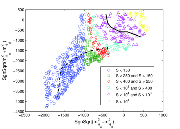
Figure 1: The bounce action for tunneling to a stau UFB-3 direction or a CCB-4 minimum as a function of the HENS model high scale input parameters $m_{H_{u}}^{2}(M_{c})$ and $m_{H_{d}}^{2}(M_{c})$ for $m_{1/2}=500\,\,{\rm GeV}$ and $\tan\beta=30$. All points shown are consistent with collider phenomenology. The points enclosed below by the dash-dot line have a neutralino LSP. The solid line separates the region with a CCB-4 minimum or saddle point (left) from that which only has a UFB-3 (right). $S>400$ is cosmologically safe.

We first consider the cases with $\tan\beta=30$, where the tau Yukawa coupling is enhanced. This has the effect of opening up a CCB-4 minimum or CCB-4-like saddle point that flows to a UFB-3 direction. In Fig. 1 we show ranges of the bounce action for tunneling out of the SM vacuum to a CCB-4 minimum or a UFB-3 direction for $m_{1/2}=500\,\,{\rm GeV}$ as a function of the input values of $m_{H_{u}}^{2}(M_{c})$ and $m_{H_{d}}^{2}(M_{c})$. All points to the left of the solid line in this figure have either a CCB-4 minimum or saddle point. The points to the right have either a stable SM vacuum or a UFB-3 direction with no CCB-4 stationary point. To the left and the right of the solid line we show the bounce action for tunneling along the direction leading to the CCB-4 stationary point or to the UFB-3 direction, whichever is smaller. We emphasize the CCB-4 stationary point here, even when it is only a saddle point, because we find that the most dangerous lowest-action tunneling path from the electroweak minimum is typically one that passes near this point with $\tilde{\nu}_{L_{i\neq 3}}=0$. The dot-dashed line in Fig. 1 indicates the upper border of the portion of parameter space in which the LSP is the lightest neutralino. (See Ref. [11] for more details.). In Fig. 2 we show the same quantities as in Fig. 1 for $m_{1/2}=1000\,\,{\rm GeV}$.

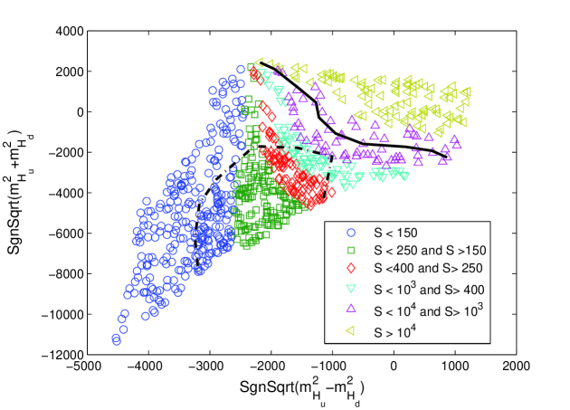
Figure 2: The bounce action for tunneling to a stau UFB-3 direction or a CCB-4 minimum as a function of the high-scale HENS model input parameters $m_{H_{u}}^{2}(M_{c})$ and $m_{H_{d}}^{2}(M_{c})$ for $m_{1/2}=1000\,{\rm GeV}$, $\tan\beta=30$ and $sgn(\mu)=1$. All points shown are consistent with collider phenomenology. The points enclosed below by the dash-dot line have a neutralino LSP. The solid line separates the region with a CCB-4 minimum or saddle point (left) from that which only has a UFB-3 direction. $S>400$ is cosmologically safe.

Both Fig. 1 and Fig. 2 show that for $\tan\beta=30$ the lifetime for tunneling to a stau UFB-3 direction or CCB-4 minimum is shorter than the age of the universe, corresponding to $S_{b}<400$, over a large portion of the otherwise acceptable parameter space. As expected, the newly disallowed regions are those with large and negative values of $m_{H_{u}}^{2}$ and $m_{H_{d}}^{2}$ at the input scale $M_{c}$. Of these two soft masses, only $m_{H_{u}}^{2}$ appears in the potential relevant for the UFB-3 direction or the CCB-4 minimum, and it has the stronger effect. Indeed, the isocontours of $S_{b}$ coincide roughly with lines of constant $m_{H_{u}}^{2}$ for smaller values of $m_{H_{d}}^{2}$. For smaller values of $m_{H_{u}}^{2}$ the SM vacuum becomes sufficiently long-lived to describe our universe. The bounce action for these points is much larger simply because the effective width of the barrier is larger. Note that this stable region includes the minimal gaugino mediation point, $m_{H_{u}}^{2}=m_{H_{d}}^{2}=0$ at $M_{c}$.

Comparing the plots for $m_{1/2}=500\,\,{\rm GeV}$ and $m_{1/2}=1000\,\,{\rm GeV}$, we see that larger $m_{1/2}$ tends to yield a slightly more stable SM vacuum. This arises simply because increasing the input gaugino masses also increases the low-scale slepton soft masses through RG running. On the other hand, larger gaugino masses also permit more negative values of $m_{H_{u}}^{2}$, so there remain significant parameter regions in which the tunneling rate is too fast. From Fig. 1, where $m_{1/2}=500\,\,{\rm GeV}$, we see that nearly the entire region in which the lightest superpartner is a neutralino is ruled out by our vacuum stability considerations. For $m_{1/2}=1000\,\,{\rm GeV}$, there is a small region in which the lightest superpartner is a neutralino and the electroweak vacuum is sufficiently long-lived.

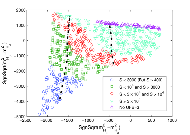
Figure 3: The bounce action for tunneling to a stau UFB-3 direction as a function of the HENS model parameters $m_{H_{u}}^{2}$ and $m_{H_{d}}^{2}$. The other HENS parameters have been fixed to be $m_{1/2}=500\,{\rm GeV}$, $\tan\beta=10$, and $sgn(\mu)=1$. All points shown are consistent with collider phenomenology. The points between the two dash-dotted lines have a neutralino LSP. $S>400$ is cosmologically safe.

We turn next to the cases with $\tan\beta=10$, for which the tau Yukawa coupling is less enhanced. In Figs. 3 and 4 we show ranges of the bounce action for tunneling from the SM vacuum to the UFB-3 direction for $\tan\beta=10$ and $M_{1/2}=500,\,300\,\,{\rm GeV}$ as a function of the input values of $m_{H_{u}}^{2}$ and $m_{H_{d}}^{2}$ at $M_{c}$. No CCB-4 local extremum is found for any of the points scanned over since the deviation from $F$-flatness is a sizeable effect in this case. The dot-dashed lines in these plots enclose the portion of parameter space in which the LSP is the lightest neutralino. (See Ref. [11] for more details.) From these plots we see that the lifetime of the standard electroweak vacuum against tunneling to a UFB-3 direction is safely large for both $m_{1/2}=500,\,300\,\,{\rm GeV}$. This is the result of the smaller value of the tau Yukawa coupling $y_{\tau}$, which gives rise to a larger barrier against tunneling, Eq. (5). As before, with all else equal $S_{b}$ increases with $m_{1/2}$ and so higher values of $m_{1/2}$ remain safe.

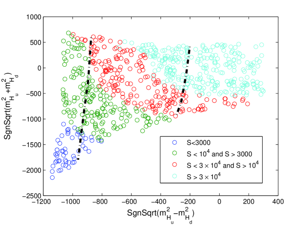
Figure 4: The bounce action for tunneling to a stau UFB-3 direction as a function of the HENS model parameters $m_{H_{u}}^{2}$ and $m_{H_{d}}^{2}$. The other HENS parameters have been fixed to be $m_{1/2}=300\,{\rm GeV}$, $\tan\beta=10$, and $sgn(\mu)=1$. All points shown are consistent with collider phenomenology. The points between the two dash-dot lines have a neutralino LSP. $S>400$ is cosmologically safe.

At smaller values of $\tan\beta$ the top quark Yukawa coupling grows larger, and we should check that the tunneling rate to CCB-4 minima associated with the stops is adequately small. As was previously discussed, this direction will only occur if $m_{H_{d}}^{2}$ is large and negative. In Fig. 5 we show contours of the bounce action for tunneling to the stop CCB-4 minimum, as well as the regions in which the SM minimum is the true minimum. Only a very few points at the largest and most negative values of $m_{H_{d}}^{2}$ are excluded, while in the great majority of the parameter space the SM vacuum is the true minimum. We find a similar result for $m_{1/2}=300\,\,{\rm GeV}$.

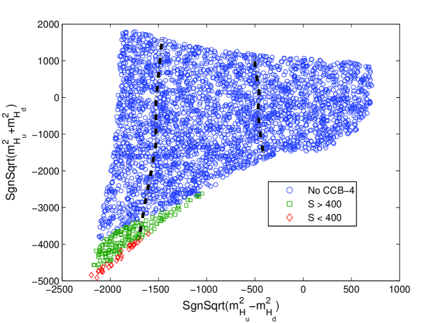
Figure 5: The bounce action for tunneling to a stop CCB-4 minimum as a function of the HENS model parameters $m_{H_{u}}^{2}$ and $m_{H_{d}}^{2}$. The other HENS parameters are $m_{1/2}=500\,{\rm GeV}$, $\tan\beta=10$ and $sgn(\mu)=1$. All these points are consistent with collider phenomenology. The points between the two dash-dot lines have a neutralino LSP. $S>400$ is cosmologically safe.

5 Conclusion

In the present work we have examined the constraints placed on the HENS model from vacuum stability. Due to the large tachyonic Higgs soft masses that can emerge in this model, there often arise local vacuum states deeper than the standard electroweak minimum. Many points that are consistent with collider phenomenological constraints (described in Ref. [11]) are ruled out because they lead to an overly short-lived SM vacuum.

The most dangerous vacuum feature is a UFB-3 direction involving the stau fields. We have also found a new CCB-4 saddle point that facilitates tunneling to the UFB-3 direction. As a result, vacuum tunneling rates tend to be too fast for larger values of $\tan\beta$. At lower values of $\tan\beta$, tunneling to a CCB-4 direction involving stop fields rules out a very small portion of the parameter space, with the rest of the parameter space being safely long-lived.

We conclude that the HENS models with a neutralino LSP and larger values of $\tan\beta=30$ are mostly ruled out subject to our assumptions about the input scale and gaugino mass universality. On the other hand, minimal gaugino mediation and the HENS models without a neutralino LSP may still have a sufficiently long-lived electroweak vacuum state at larger values of $\tan\beta$. For lower values of $\tan\beta$, such as $\tan\beta=10$, the constraints from vacuum tunneling are much weaker, and most of the parameter space that is consistent with collider lower-energy bounds remains viable.

Appendix A Appendix: The Improved Action Method

The bounce action is a stationary point of the Euclidean action given in Eq. (9) subject to the boundary conditions of Eqs. (10,11). The corresponding equations of motion for the $O(4)$ symmetric solution are

$$\frac{d^{2}\bar{\phi}_{i}}{d\rho^{2}}+\frac{3}{\rho}\frac{d\bar{\phi}_{i}}{d\rho}=\frac{\partial}{\partial\bar{\phi}_{i}}U(\bar{\phi}_{i}).$$ (12)

where $i$ runs over the independent fields. These equations are a set of non-linear coupled differential equations with an a priori unknown starting point. These conditions together make it a very difficult problem to solve and require numerical techniques [17, 32, 33].

The technique we use in the present work is called the improved action method [32]. In this method, additional terms are added to the action that are identically zero for the bounce solution. The advantage of adding these terms is that they make the bounce solution a minimum of this modified action and not just an extremum. The term that does this is found by making the change of variable $x\to\sigma x$ in Eq. (9). Because the bounce is the extremum of the action, the first derivative of the scaled action with respect to $\sigma$ will be zero for $\sigma=1$. This gives the following condition:

$$\left(\sigma^{2}T[\bar{\phi}_{i}]+2\sigma^{4}U[\bar{\phi}_{i}]\right)|_{\sigma=1}=0$$ (13)

This relation illustrates that the potential term must be negative. The kinetic term cannot be negative because it is the integral of a sum of squares. Since the potential term scales as $\sigma^{4}$ and the kinetic term scales as $\sigma^{2}$, Eq. (13) defines a maximum. Thus, we have determined the maximal direction of the saddle point. By adding to the action the absolute value of this quantity to a positive power, the saddle point of the action can be turned into a minimum. In this case the improved action is

$$S[\bar{\phi}_{i}]=T[\bar{\phi}_{i}]+U[\bar{\phi}_{i}]+\lambda\left|T[\bar{\phi}_{i}]+2U[\bar{\phi}_{i}]\right|^{n}$$ (14)

where $\lambda$ and $n$ are positive constants.

To solve for the bounce with this improved action, we take an initial profile for the vevs $\phi_{i}$ with the kinetic and potential terms

$$T[\phi_{i}]=2\pi^{2}\Delta^{4}\sum_{m=1}^{L-1}(\rho_{m+1}-\rho_{m})\rho_{m}^{3}\left[\sum_{i}^{n}\frac{(\phi_{i}^{m+1}-\phi_{i}^{m})^{2}}{2(\rho_{m+1}-\rho_{m})^{2}\Delta^{2}}\right]$$ (15)

$$U[\phi_{i}]=2\pi^{2}\Delta^{4}\sum_{m=1}^{L-1}(\rho_{m+1}-\rho_{m})\rho_{m}^{3}U(\phi_{1}^{m},...,\phi_{n}^{m}).$$ (16)

$\Delta$ is a parameter determined by Eq. (13). Inspired by the thin-wall approximation, we take the following initial guess for the bounce solution

$$\phi(\rho)=a\tanh(b(\rho-\rho_{0}))+c.$$ (17)

The coefficients $a$ and $c$ can be solved for by applying the boundary conditions $\phi(0)=\phi_{e}$ and $\phi(\infty)=\phi_{f}$, where $\phi_{f}$ are the field values in the SM minimum and $\phi_{e}$ are the values in the vacuum to which the tunneling connects. Since $\phi_{e}$ is a priori unknown, this leaves $\phi_{e}$, $b$, and $\rho_{0}$ as free parameters. These parameters are determined by first substituting the field profile in Eq. (17) into the modified action for each $\phi_{i}$.

The $\phi_{e}$ will not in general be the field configuration of the minima, but rather some field points inside the well. In the case of a UFB-3 direction there is no minimum, and $\phi_{e}$ will be some point on the runaway downslope with a potential energy less than that at SM minimum. The exact value of $\phi_{e}$ as well as $b$ and $\rho_{0}$ are determined using a minimization routine that finds the coefficients that minimize the modified action. In Ref. [20] the authors used the thick-wall approximation as an initial guess. In our case, the guess given in Eq. (13) works better numerically because it is adaptable to both thick- and thin-wall potential profiles. Once the initial profile, coefficients and all, is determined, we randomly vary each lattice site. The variations are stopped when further iterations do not reduce the modified action. To ensure that we arrive at the bounce solution, we choose a value of $\lambda$ that ensures $0.999<(-T[\phi_{i}]/2/V[\phi_{i}])^{1/2}<1.001$. The smallest value of $\lambda$ able to maintain this condition and used to optimize the code was close to $0.5$ with $n=1$.

Appendix B Appendix: Tunneling Through an Inverted Parabola

We exhibit here an exact bounce solution for a single field tunneling through an inverted parabolic potential. To the best of our knowledge, this simple solution has not been presented elsewhere in the literature, although a related solution for a linearized potential was obtained in the pioneering work of Ref. [29].

Consider the run-away potential

$$V(\phi)=a|\phi|-b|\phi|^{2},$$ (18)

where $\phi$ is a real scalar field. The origin is a metastable minimum for $a,\,b>0$. Focussing on $\phi>0$, the equation of motion for an $O(4)$-symmetric bounce is

$$\frac{d^{2}\phi}{d\rho^{2}}+\frac{3}{\rho}\,\frac{d\phi}{d\rho}+(2b\,\phi-a)=0,$$ (19)

where $\rho$ is the Euclidean distance. The boundary conditions for the bounce are

$$\frac{d\phi}{d\rho}(\rho=0) = 0$$ (20)

$$\phi(R) = 0$$ (21)

$$\frac{d\phi}{d\rho}(\rho=R) = 0$$ (22)

For potentials in which the false vacuum is flat, $R\to\infty$, as we assumed in Eq. (11). Here, the potential has a singular first derivative at the false vacuum at the origin. As a result, the bounce reaches the origin at finite $R$ and remains there asymptotically [34]. We have checked that deforming the potential into a concave parabola very near the origin to resolve this singularity leads to $R\to\infty$, but otherwise has only a small (and smooth) effect on the solution presented here away from the origin.

Eq. (19) is a linear second-order differential equation that can be solved analytically. The general solution before imposing boundary conditions is

$$\phi(\rho)=\frac{a}{2b}+\frac{1}{x}\left[c_{1}\,J_{1}(x)+c_{2}\,Y_{1}(x)\right],$$ (23)

where $J_{1}$ and $Y_{1}$ are Bessel functions of the first kind,

$$x=\frac{\rho}{\sqrt{2b}},$$ (24)

and $c_{1}$ and $c_{2}$ are constant coefficients. The values of $c_{1}$ and $c_{2}$, as well as $R$, are fixed by the boundary conditions, Eqs. (20-22). The first of these, Eq. (20), gives

$$0 = \left.\frac{d}{dx}\left(\frac{1}{x}\left[c_{1}J_{1}(x)+c_{2}Y_{1}(x)\right]\right)\right|_{x=0}$$ (25)

$$= -\lim_{x\to 0}\left(\frac{1}{x}\left[c_{1}J_{2}(x)+c_{2}\,Y_{2}(x)\right]\right),$$

where we have made use of the recursion properties of Bessel functions [35]. For this limit to be non-singular, we must have $c_{2}=0$. On the other hand, $J_{2}(x)/x$ vanishes at the origin so no constraint is imposed on $c_{1}$ by this condition. Applying Eq. (22), we find

$$0 = c_{1}\left.\frac{d}{dx}\left[\frac{1}{x}J_{1}(x)\right]\right|_{x=x_{+}}$$

$$= -c_{1}\,\frac{1}{x_{+}}J_{2}(x_{+}),$$

where we have defined $x_{+}=R/\sqrt{2b}$. From this, we conclude that $x_{+}$ must be a zero of $J_{2}$. In particular, for the minimal action bounce solution, it should be the first non-trivial zero:

$$x_{+}\simeq 5.1356\ldots$$ (27)

Finally, let us apply the condition of Eq. (21) to fix $c_{1}$,

$$c_{1}=-\frac{a}{2b}\left[\frac{x_{+}}{J_{1}(x_{+})}\right].$$ (28)

We can use this exact solution to compute several interesting quantities related to the bounce. The bounce action is found to be

$$S_{E} = 2\pi^{2}\int_{0}^{R}d\rho\,\rho^{3}\left[\frac{1}{2}\left(\frac{d\phi}{d\rho}\right)^{2}+V(\phi)\right]$$

$$= \frac{\pi^{2}}{32}\,x_{+}^{4}\,\frac{a^{2}}{b^{3}}$$

$$\simeq (215)\,\frac{a^{2}}{b^{3}}.$$

The value of the field $\phi$ at the escape point where it emerges from tunneling is given by

$$\phi(0)=\frac{a}{2b}-\frac{a}{2b}\left[\frac{x_{+}}{J_{1}(x_{+})}\right]\,\lim_{x\to 0}\frac{J_{1}(x)}{x}\simeq\frac{4a}{b}.$$ (30)

For comparison, the maximum of the potential occurs at $\phi=a/2b$ and the width of the potential barrier is $\Delta\phi=a/b$. Thus, the escape point is well beyond the peak, but only by a factor of a few.

The exact solution presented here can also be extended to potentials that are piecewise segments of parabolas, in analogy to the solution for piecewise-linear potentials presented in Ref. [34]. (When the local potential is a concave parabola, the general local solution consists of modified Bessel functions of the first kind.) This offers the possibility of obtaining closed-form expressions for bounce solutions to a wide variety of potentials by approximating them with segments of parabolas. In practice, we find that the matching conditions between adjacent parabolic segments often lead to complicated implicit transcendental equations. The generalization to thermal transitions over piecewise-parabolic barriers is also straightforward.

References

-
[1]
For general reviews, see:
S. P. Martin, hep-ph/9709356; D. J. H. Chung, L. L. Everett, G. L. Kane, S. F. King, J. D. Lykken and L. T. Wang, Phys. Rept. 407, 1 (2005) [hep-ph/0312378]. - [2] F. Gabbiani, E. Gabrielli, A. Masiero and L. Silvestrini, Nucl. Phys. B 477, 321 (1996) [arXiv:hep-ph/9604387]. M. Misiak, S. Pokorski and J. Rosiek, Adv. Ser. Direct. High Energy Phys. 15, 795 (1998) [arXiv:hep-ph/9703442].
- [3] For a review, see A. B. Lahanas and D. V. Nanopoulos, Phys. Rept. 145, 1 (1987); A. B. Lahanas, “No scale supergravity: A Viable scenario for understanding the SUSY CERN-TH-7092-93 Lectures given at International School of Subnuclear Physics: 31th Course: From Supersymmetry to the Origin of Space-Time, Erice, Italy, 4- 12 Jul 1993
- [4] D. E. Kaplan, G. D. Kribs and M. Schmaltz, Phys. Rev. D 62, 035010 (2000) [hep-ph/9911293]; Z. Chacko, M. A. Luty, A. E. Nelson and E. Ponton, JHEP 0001, 003 (2000) [hep-ph/9911323].
- [5] A. E. Nelson and M. J. Strassler, JHEP 0009, 030 (2000) [arXiv:hep-ph/0006251]; A. E. Nelson and M. J. Strassler, “Exact results for supersymmetric renormalization and the supersymmetric JHEP 0207, 021 (2002) [arXiv:hep-ph/0104051].
- [6] M. A. Luty and R. Sundrum, Phys. Rev. D 65, 066004 (2002) [arXiv:hep-th/0105137]. M. Luty and R. Sundrum, Phys. Rev. D 67, 045007 (2003) [arXiv:hep-th/0111231]. M. Ibe, K. I. Izawa, Y. Nakayama, Y. Shinbara and T. Yanagida, Phys. Rev. D 73, 015004 (2006) [arXiv:hep-ph/0506023]. M. Ibe, K. I. Izawa, Y. Nakayama, Y. Shinbara and T. Yanagida, Phys. Rev. D 73, 035012 (2006) [arXiv:hep-ph/0509229]. M. Schmaltz and R. Sundrum, arXiv:hep-th/0608051.
- [7] M. Dine, P. J. Fox, E. Gorbatov, Y. Shadmi, Y. Shirman and S. D. Thomas, Phys. Rev. D 70, 045023 (2004) [arXiv:hep-ph/0405159].
- [8] A. G. Cohen, T. S. Roy and M. Schmaltz, JHEP 0702, 027 (2007) [arXiv:hep-ph/0612100]; T. S. Roy and M. Schmaltz, Phys. Rev. D 77, 095008 (2008) [arXiv:0708.3593 [hep-ph]].
- [9] H. Murayama, Y. Nomura and D. Poland, Phys. Rev. D 77, 015005 (2008) [arXiv:0709.0775 [hep-ph]].
- [10] G. Perez, T. S. Roy and M. Schmaltz, arXiv:0811.3206 [hep-ph].
- [11] J. L. Evans, D. E. Morrissey and J. D. Wells, Phys. Rev. D 75, 055017 (2007) [arXiv:hep-ph/0611185].
- [12] M. Schmaltz and W. Skiba, Phys. Rev. D 62, 095005 (2000) [arXiv:hep-ph/0001172]; M. Schmaltz and W. Skiba, Phys. Rev. D 62, 095004 (2000) [arXiv:hep-ph/0004210].
- [13] W. Buchmuller, J. Kersten and K. Schmidt-Hoberg, JHEP 0602, 069 (2006) [arXiv:hep-ph/0512152]; W. Buchmuller, L. Covi, J. Kersten and K. Schmidt-Hoberg, arXiv:hep-ph/0609142.
- [14] S. P. Martin and M. T. Vaughn, Phys. Rev. D 50, 2282 (1994) [Erratum-ibid. D 78, 039903 (2008)] [arXiv:hep-ph/9311340].
- [15] D. E. Kaplan and T. M. P. Tait, JHEP 0006, 020 (2000) [arXiv:hep-ph/0004200].
- [16] J. F. Gunion, H. E. Haber and M. Sher, Nucl. Phys. B 306, 1 (1988).
- [17] M. Claudson, L. J. Hall and I. Hinchliffe, Nucl. Phys. B 228, 501 (1983).
- [18] J. A. Casas, A. Lleyda and C. Munoz, Nucl. Phys. B 471, 3 (1996) [arXiv:hep-ph/9507294].
- [19] A. Riotto and E. Roulet, Phys. Lett. B 377, 60 (1996) [arXiv:hep-ph/9512401].
- [20] A. Kusenko, P. Langacker and G. Segre, Phys. Rev. D 54, 5824 (1996) [arXiv:hep-ph/9602414].
- [21] J. R. Ellis, J. Giedt, O. Lebedev, K. Olive and M. Srednicki, Phys. Rev. D 78, 075006 (2008) [arXiv:0806.3648 [hep-ph]].
- [22] M. Quiros, Helv. Phys. Acta 67, 451 (1994).
- [23] M. S. Carena, M. Quiros and C. E. M. Wagner, Phys. Lett. B 380, 81 (1996) [arXiv:hep-ph/9603420]; M. Carena, G. Nardini, M. Quiros and C. E. M. Wagner, arXiv:0809.3760 [hep-ph].
- [24] M. Dine, L. Randall and S. D. Thomas, Phys. Rev. Lett. 75, 398 (1995) [arXiv:hep-ph/9503303].
- [25] S. Komine and M. Yamaguchi, Phys. Rev. D 63, 035005 (2001) [arXiv:hep-ph/0007327].
- [26] C. Balazs and R. Dermisek, JHEP 0306, 024 (2003) [arXiv:hep-ph/0303161].
- [27] J. R. Ellis, K. A. Olive and Y. Santoso, Phys. Lett. B 539, 107 (2002) [arXiv:hep-ph/0204192]; J. R. Ellis, T. Falk, K. A. Olive and Y. Santoso, Nucl. Phys. B 652, 259 (2003) [arXiv:hep-ph/0210205];
- [28] H. Baer, A. Mustafayev, S. Profumo, A. Belyaev and X. Tata, JHEP 0507, 065 (2005) [arXiv:hep-ph/0504001].
- [29] S. R. Coleman, Phys. Rev. D 15, 2929 (1977) [Erratum-ibid. D 16, 1248 (1977)].
- [30] C. G. . Callan and S. R. Coleman, Phys. Rev. D 16, 1762 (1977).
- [31] S. R. Coleman, V. Glaser and A. Martin, Commun. Math. Phys. 58, 211 (1978).
- [32] A. Kusenko, Phys. Lett. B 358, 51 (1995) [arXiv:hep-ph/9504418];
- [33] T. Konstandin and S. J. Huber, JCAP 0606, 021 (2006) [arXiv:hep-ph/0603081].
- [34] M. J. Duncan and L. G. Jensen, Phys. Lett. B 291, 109 (1992).
- [35] J. Mathews and R.L. Walker, Mathematical Methods of Physics (Addison, 1970).