Statistical physics of a model binary genetic switch with linear feedback

Abstract

We study the statistical properties of a simple genetic regulatory network that provides heterogeneity within a population of cells. This network consists of a binary genetic switch in which stochastic flipping between the two switch states is mediated by a “flipping” enzyme. Feedback between the switch state and the flipping rate is provided by a linear feedback mechanism: the flipping enzyme is only produced in the on switch state and the switching rate depends linearly on the copy number of the enzyme. This work generalises the model of [Phys. Rev. Lett., 101, 118104] to a broader class of linear feedback systems. We present a complete analytical solution for the steady-state statistics of the number of enzyme molecules in the on and off states, for the general case where the enzyme can mediate flipping in either direction. For this general case we also solve for the flip time distribution, making a connection to first passage and persistence problems in statistical physics. We show that the statistics of the model are non-Poissonian, leading to a peak in the flip time distribution. The occurrence of such a peak is analysed as a function of the parameter space. We present a new relation between the flip time distributions measured for two relevant choices of initial condition. We also introduce a new correlation measure to show that this model can exhibit long-lived temporal correlations, thus providing a primitive form of cellular memory. Motivated by DNA replication as well as by evolutionary mechanisms involving gene duplication, we study the case of two switches in the same cell. This results in correlations between the two switches; these can either positive or negative depending on the parameter regime.

I Introduction

Populations of biological cells frequently show stochastic switching between alternative phenotypic states. This phenomenon is particularly well-studied in bacteria and bacteriophages, where it is known as phase variation [1]. Phase variation often affects cell surface features, and its evolutionary advantages are believed to involve evading attack from host defense systems (e.g. the immune system) and/or “bet-hedging” against sudden catastrophes which may wipe out a particular phenotypic type. Switching between different phenotypic states is controlled by an underlying genetic regulatory network, which randomly flips between alternative patterns of gene expression. Several different types of genetic network are known to control phase variation—these include DNA inversion switches, DNA methylation switches and slipped strand mispairing mechanisms [1, 2, 3].

In this paper, we study a simple model for a genetic network that allows switching between two alternative states of gene expression. Its key feature is that it includes a linear feedback mechanism between the switch state and the flipping rate. When the switch is active, an enzyme is produced and the rate of switching is linearly proportional to the copy number of this enzyme. The statistical properties of this model are made non-trivial by this feedback, leading, among other things, to non-Poissonian behaviour that may be of advantage to cells in surviving in certain dynamical environments. Our model is very generic and does not aim to describe any specific molecular mechanism in detail, but rather to determine in a general way the consequences of the linear feedback for the switching statistics. Motivated by the fact that cells often contain multiple copies of a particular genetic regulatory element, due to DNA replication or DNA duplication events during evolution, we also consider the case of two identical switches in the same cell. We find that the two copies of the switch are coupled and may exhibit interesting and potentially important correlations or anti-correlations. Our model switch is fundamentally different from bistable gene networks that have been the subject of previous theoretical interest. In fact, as we shall show, our switch is not bistable but is intrinsically unstable in each of its two states.

Before discussing our model in detail, we provide a brief overview of the basic biology of genetic networks and summarise some previously considered models for genetic switches. Genetic networks are interacting, many-component systems of genes, RNA and proteins, that control the functions of living cells. Genes are stretches of DNA ($\sim$1000 base pairs long in bacteria), whose sequences encode particular protein molecules. To produce a protein molecule, the enzyme complex RNA polymerase copies the gene sequence into a messenger RNA (mRNA) molecule. This is known as transcription. The mRNA is then translated (by a ribosome enzyme complex) into an amino acid chain which folds to form the functional protein molecule. The production of a specific set of proteins from their genes ultimately determines the phenotypic behaviour of the cell. Phenotypic behaviour can thus be controlled by turning genes on and off. Regulation of transcription (production of mRNA) is one important way of achieving this. Transcription is controlled by the binding of proteins known as transcription factors to specific DNA sequences, known as operators, usually situated at the beginning of the gene sequence. These transcription factors may be activators (which enhance the transcription of the gene they regulate) or repressors (which repress transcription, often by preventing RNA polymerase binding). A given gene may encode a transcription factor that regulates itself or other genes, leading to complex networks of transcriptional interactions between genes.

There has been much recent interest among both physical scientists and biologists in deconstructing complex genetic networks into modular units [4], and in seeking to understand their statistical properties using theory and simulation [5, 6]. Of particular interest is the fact that genetic networks are intrinsically stochastic, due to the small numbers of molecules involved in gene expression [7, 8]. This can give rise to heterogeneity in populations of genetically and environmentally identical cells [7]. For some genetic networks, this heterogeneity is “all-or-nothing”: the population splits into two distinct sub-populations, with different states of gene expression. Such networks are known as bistable genetic switches: they have two possible long-time states, corresponding to alternative phenotypic states. Well-known examples are the switch controlling the transition from the lysogenic to lytic states in bacteriophage $\lambda$ [9, 10], and the lactose utilisation network of the bacterium Escherichia coli [11]. Several simple mechanisms for achieving bistability have been studied, including pairs of mutually repressing genes [13, 12], positive feedback loops [14] and mixed feedback loops [15]. Such bistable genetic networks can allow long-lived and binary responses to short-lived signals—for example, when a cell is triggered by a transient signal to commit to a particular developmental pathway.

Theoretical treatments of bistable genetic networks usually consider the dynamics of the copy number (or concentration) of the regulatory proteins involved. This affects the activation state of the genes, which in turn influences the rate of protein production. The macroscopic rate equation approach [16] provides a deterministic (mean-field) description of the dynamics that ignores fluctuations in protein copy number or gene expression state. This approach, applied to a switch with two mutually repressing genes, has shown that co-operative binding of regulatory proteins is an important factor in generating bistability [13]. Other studies have shown, however, that bistability can be achieved even when the deterministic equations have only one solution, due to stochasticity and fluctuations in protein numbers [17, 18]. An alternative approach is to study the dynamics of stochastic flipping between two stable states using stochastic simulations [19, 20, 21], by numerically integrating the master equation [22], or by path integral-type approaches [23]. This dynamical problem bears some resemblance to the Kramers problem of escape from a free energy minimum [24, 25], and one expects on general grounds that the typical time spent in one of the bistable states should be exponentially large in the typical number of proteins present in the state. This has been confirmed, at least for cooperative toggle switches formed of mutually repressing genes [19, 20]. From the perspective of statistical physics, interesting questions arise concerning the distribution of escape times and the connection to first passage properties of stochastic processes.

In this paper, however, we are concerned with an intrinsically different situation from these bistable genetic networks. The molecular mechanisms controlling microbial phase variation typically involve a binary element that can be in either of two states. For example, this may be a short fragment of DNA that can be inserted into the chromosome in either of two orientations, a repeated DNA sequence that can be altered in its number of repeats, or a DNA sequence that can have two alternative patterns of methylation [1]. The flipping of this element between its two states is stochastic, with a flipping rate that is controlled by various regulatory proteins, the activity of which may be influenced by environmental factors. We shall consider the case where a feedback exists between the switch state and the flipping rate. This is particularly interesting from a statistical physics point of view because it leads to non-Poissonian switching behaviour, as we shall show. Our work has been motivated by several examples. The fim system in uropathogenic strains of the bacterium E. coli controls the production of Type 1 fimbriae (or pili), which are “hairs” on the surface of the bacterium. Individual cells switch stochastically between “on” and “off” states of fimbrial production [1, 26, 27, 28]. The key feature of the fim switch is a short piece of DNA that can be inserted into the bacterial DNA in two possible orientations. Because this piece of DNA contains the operator sequence for the proteins that make up the fimbriae, in one orientation, the fimbrial genes are transcribed and fimbriae are produced (the “on” state) and in the other orientation, the fimbrial genes are not active and no fimbriae are produced (the “off” state). The inversion of this DNA element is mediated by recombinase enzymes. Feedback between the switch state and the switch flipping rate arises because the FimE recombinase (which flips the switch in the on to off direction), is produced more strongly in the on switch state than in the off state. This phenomenon is known as orientational control [29, 30, 31]. The production of a second type of fimbriae in uropathogenic E. coli, Pap pili, also phase varies, and is controlled by a DNA methylation switch [1, 2, 32]. Here, the operator region for the genes encoding the Pap pili can be in two states, in which the DNA is chemically modified (methylated) at different sites, and different binding sites are occupied by the regulatory protein Lrp. Switching in this system is facilitated by the PapI protein, which helps Lrp to bind [33]. Feedback between the switch state and the flipping rate arises because the production of PapI itself is activated by the protein PapB, which is only produced in the “on” state [34, 1, 2].

A common feature of the above examples is the existence of a feedback mechanism: in the fim system this occurs through orientational control, and in the pap system, through activation of the papI gene by PapB. In this paper, we aim to study the role of such feedback within a simple, generic model of a binary genetic switch. We shall assume that the feedback is linear, and we thus term our model a “linear feedback switch”. In a recent publication [35], we introduced a simple mathematical model of a DNA inversion genetic switch with orientational control, which was inspired by the fim system. Our model reduces to the dynamics of the number of molecules of a “flipping enzyme” $R$, which mediates switch flipping, along with a binary switch state. Enzyme $R$ is produced only in the on switch state. As the copy number of $R$ increases, the on to off flipping rate of the switch increases and this results in a non-Poissonian flipping process with a peak in the lifetime of the on state. The model is linear in the sense that the rate at which the switch is turned off is a linear function of the number of enzymes $R$ which it produces. In our previous work [35], we imagined enzyme $R$ to be a DNA recombinase, and the two switch states to correspond to different DNA orientations, in analogy with the fim system. However, the same model could be used to describe a range of molecular mechanisms for binary switch flipping with feedback between the switch state and flipping rate, and can thus be considered a generic model of a genetic switch with linear feedback.

In our recent work [35], we obtained exact analytical expressions for the steady state enzyme copy number for our model switch with linear feedback, in the particular case where the flipping enzyme switches only in the on to off direction (this being the relevant case for fim). We also calculated the flip time distribution for this model analytically. Conceptually, such a calculation is reminiscent of the study of persistence in statistical physics [36] where, for example, one asks about the probability that a spin in an Ising system has not flipped up to some time [37]. For the flip time distribution, we introduced different measurement ensembles according to whether one starts the time measurement from a flip event (the Switch Change Ensemble) or from a randomly selected time (the Steady State Ensemble). In the present paper, we extend this work to present the full solution of the general case of the model and extend our study of its persistence properties. The introduction of a rate for the enzyme mediated off to on flipping ($k^{\textrm{off}}_{3}$) has most significant effects on the flip time distributions $F(T)$, as illustrated in Figs. 6 and 7 where we show the parameter range over which a peak is found in $F(T)$ for zero and non-zero $k^{\textrm{off}}_{3}$. We also prove an important relation between the two measurement ensembles defined in [35] and use it to show that a peak in the flip time distribution only occurs in the Switch Change Ensemble and not in the Steady State Ensemble. We find that the non-Poissonian behaviour of this model switch leads to interesting two-time autocorrelation functions. We also study the case where we have two copies of the switch in the same cell and find that these two copies may be correlated or anticorrelated, depending on the parameters of the model, with potentially interesting biological implications.

The paper is structured as follows. In section II we define the model, describe its phenomenology, and show that a “mean-field”, deterministic version of the model has only one steady state solution. In section III we present the general solution for the steady state statistics and in section IV we study first passage-time properties of the switch; technical calculations are left to the appendices. In section V we consider two coupled model switches and we present our conclusions in section VI.

II The model

We consider a model system with a flipping enzyme $R$ and a binary switch $S$, which can be either on or off (denoted respectively as $S_{\textrm{on}}$ and $S_{\textrm{off}}$). Enzyme $R$ is produced (at rate $k_{2}$) only when the switch is in the on state, and is degraded at a constant rate $k_{1}$, regardless of the switch state. This represents protein removal from the cell by dilution on cell growth and division, as well as specific degradation pathways. Switch flipping is assumed to be a single step process, which can either be catalysed by enzyme $R$, with rate constants $k^{\textrm{on}}_{3}$ and $k^{\textrm{off}}_{3}$ and linear dependence on the number of molecules of $R$, or can happen “spontaneously”, with rates $k^{\textrm{on}}_{4}$ and $k^{\textrm{off}}_{4}$. We imagine that the “spontaneous” switching process may in fact be catalysed by some other enzyme whose concentration remains constant and which is therefore not modelled explicitly here. Our model, which is shown schematically in Fig. 1, is defined by the following set of biochemical reactions:

$$R \stackrel{{\scriptstyle k_{1}}}{{\longrightarrow}}\emptyset S_{\textrm{on}} \stackrel{{\scriptstyle k_{2}}}{{\longrightarrow}}S_{\textrm{on}}+R$$ (1a)

$$S_{\textrm{on}}+R \xrightleftharpoons[k^{\textrm{off}}_{3}]{k^{\textrm{on}}_{3}}S_{\textrm{off}}+R S_{\textrm{on}} \xrightleftharpoons[k^{\textrm{off}}_{4}]{k^{\textrm{on}}_{4}}S_{\textrm{off}}\,\,.$$ (1b)

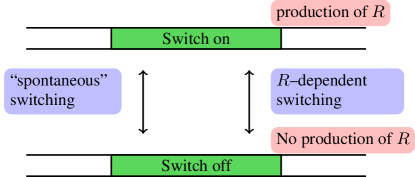
Figure 1: (colour online) A schematic illustration of the model DNA inversion switch.

II.1 Phenomenology

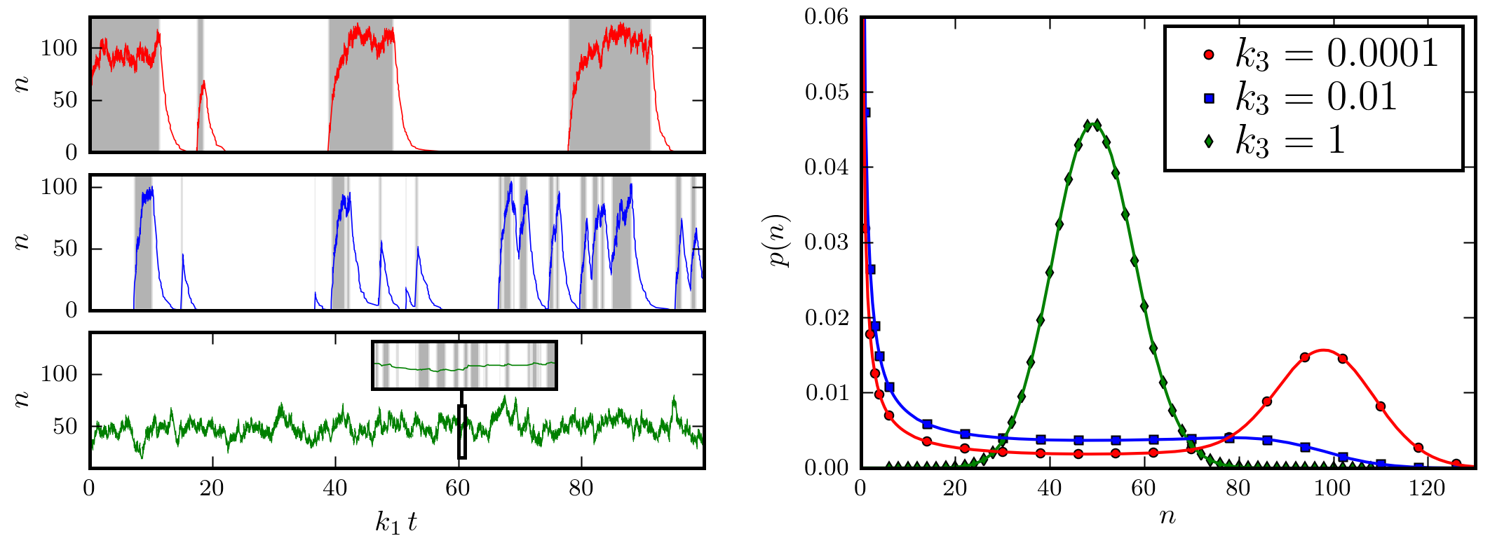
Figure 2: (colour online) Left: Typical trajectories of the system when $k^{\textrm{on}}_{3}=k^{\textrm{off}}_{3}=k_{3}$ is increased (from top to bottom $k_{3}=0.0001$, 0.01 and 1). The other parameters are $k_{1}=1$, $k_{2}=100$ and $k^{\textrm{on}}_{4}=k^{\textrm{off}}_{4}=k_{4}=0.1$. Grey shading denotes periods in which the switch is in the on state, and the solid lines denote the number of enzyme molecules, plotted against time. In the bottom panel, the switch flips so fast that the grey shading is only shown in the inset where the trajectory from $k_{1}t=[60,61]$ is shown in detail. Right: Probability distribution functions for the number $n$ of $R$ molecules, for parameter values corresponding to the trajectories shown in the left panels. The symbols are the result of numerical simulations (see text for details). The full curves plot the analytical results Eqs. (26) and (36), which are in perfect agreement with the simulations.

We notice that there are two physically relevant and coupled timescales for our model switch: the timescale associated with changes in the number of $R$ molecules (dictated by the production and decay rates $k_{1}$ and $k_{2}$), and that associated with the flipping of the switch (dictated by $k_{3}$, $k_{4}$ and the $R$ concentration).

We first consider the case where the timescale for $R$ production/decay is much faster than the switch flipping timescale. The top left panel of Fig. 2 shows a typical dynamical trajectory for parameters in this regime. Here, we plot the number $n$ of $R$ molecules, together with the switch state, against time. This result was obtained by stochastic simulation of reaction set (1) using the Gillespie algorithm [38, 39]. This algorithm generates a continuous time Markov process which is exactly described by the master equation (10). For a given switch state, the number $n$ of molecules of $R$ varies according to reactions (1a). When the switch is in the on state, $n$ grows towards a plateau value, and when the switch is in the off state, $n$ decreases exponentially towards $n=0$. The time evolution of $n$ can thus be seen as a sequence of relaxations towards two different asymptotic steady states, which depend on the switch position. To better understand this limiting case, we can make the assumption that the number of $R$ molecules evolves deterministically for a given switch state. We can then write down deterministic rate equations corresponding to the reaction scheme (1). These equations are first order differential equations for $\rho$, the mean concentration of the enzyme. When the switch is on, the rate equation reads

$$\frac{d\rho}{dt}=-k_{1}\rho+k_{2}$$ (2)

with solution

$$\rho(t)=\rho(0)e^{-k_{1}t}+\frac{k_{2}}{k_{1}}\left[1-{e}^{-k_{1}t}\right]\;.$$ (3)

Thus the plateau density in the on state is given by the ratio

$$\rho_{\rm on}=k_{2}/k_{1}\;,$$ (4)

and the timescale for relaxation to this density is given by $k_{1}$, the rate of degradation of $R_{1}$. When the switch is in the off state, the rate equation for $\rho$ reads instead

$$\frac{d\rho}{dt}=-k_{1}\rho$$ (5)

and one simply has exponential decay to $\rho=0$ with decay time $k_{1}$. In this parameter regime, switch flipping typically happens when the number of molecules of $R$ has already reached the steady state (as in the top left panel of Fig. 2). Thus, the on to off switching timescale is given by $1/(\rho_{\textrm{on}}k^{\textrm{on}}_{3}+k^{\textrm{on}}_{4})$, where $\rho_{\rm on}$ is the plateau concentration of flipping enzyme when the switch is in the on state, given by Eq.(4). Since the corresponding plateau concentration in the off switch state is zero, the off to on switch flipping timescale is simply given by $1/k^{\textrm{off}}_{4}$.

We now consider the opposite scenario, in which switching occurs on a much shorter timescale than relaxation of the enzyme copy number. A typical trajectory for this case is shown in the bottom left panel of Fig. 2. Here, switching reactions dominate the dynamics of the model, and the dynamics of the enzyme copy number follows a standard birth-death process, with an effective birth rate given by the enzyme production rate in the on state multiplied by the fraction of time spent in the on state. A more quantitative account for these behaviours is provided later on, in III.2.

For parameter values between these two extremes, where the timescales for switch flipping and enzyme number relaxation are similar, it is more difficult to provide intuitive insights into the behaviour of the model. A typical trajectory for this case is given in the middle left panel of Fig. 2. Here, we have set the on to off and off to on switching rates to be identical: $k^{\textrm{on}}_{3}=k^{\textrm{off}}_{3}$ and $k^{\textrm{on}}_{4}=k^{\textrm{off}}_{4}$. We notice that typically, less time is spent in the on state than in the off state. As soon as the switch flips into the on state, the number of $R$ molecules starts increasing and the on to off flip rate begins to increase. Consequently, the number of $R$ molecules rarely reaches its plateau value before the switch flips back into the off state.

To illustrate the effects of including the parameter $k^{\textrm{off}}_{3}$, we also show trajectories for different values of the ratio $r=k^{\textrm{off}}_{3}/k^{\textrm{on}}_{3}$ in Fig. 3, for fixed $k^{\textrm{on}}_{3}$. For small $r$, the amount of enzyme decays to zero in the off state before the next off-to-on flipping event resulting in bursts of enzyme production. In contrast, when $r$ is $O(1)$, flipping is rapid in both directions so that $p(n)$ is peaked at intermediate $n$.

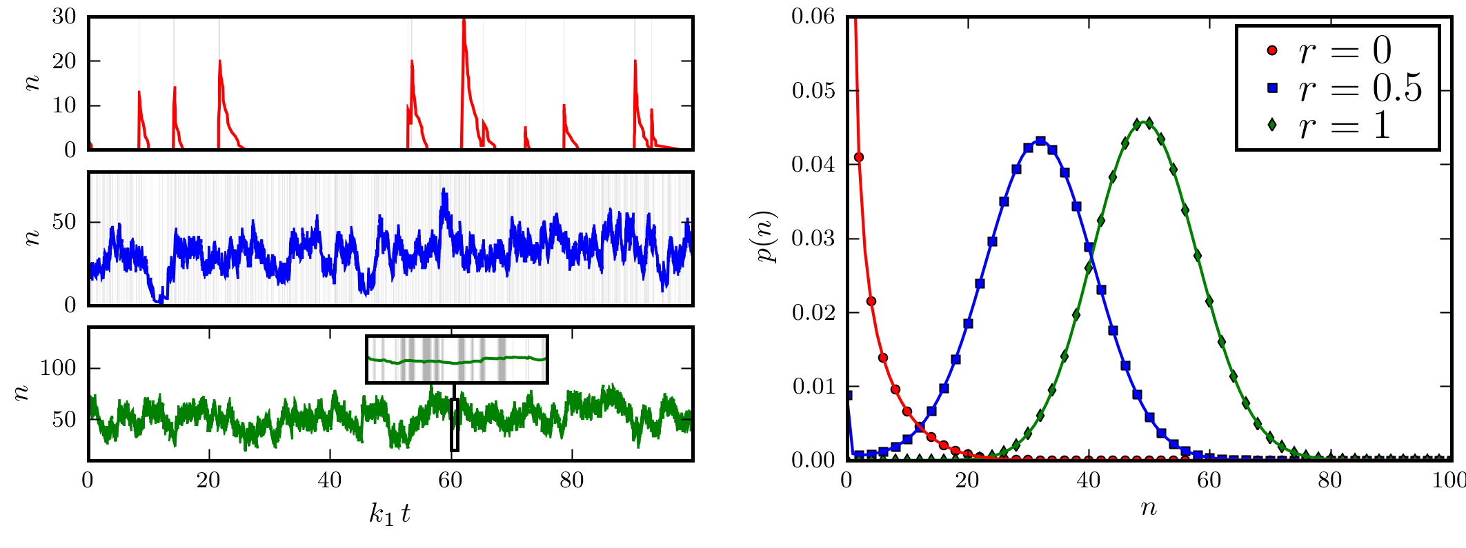
Figure 3: (colour online) Left: Typical trajectories of the system when $r=k^{\textrm{off}}_{3}/k^{\textrm{on}}_{3}=$ is increased (from top to bottom $r=0$, 0.5 and 1). The other parameters are $k_{1}=1$, $k_{2}=100$, $k^{\textrm{on}}_{3}=1$ and $k^{\textrm{on}}_{4}=k^{\textrm{off}}_{4}=k_{4}=0.1$. Grey shading denotes periods in which the switch is in the on state, and the solid lines denote the number of enzyme molecules, plotted against time. In the bottom panel, the switch flips so fast that the grey shading is only shown in the inset where the trajectory from $k_{1}t=[60,61]$ is shown in detail. Right: Probability distribution functions for the number $n$ of $R$ molecules, for parameter values corresponding to the trajectories shown in the left panels. The symbols are the result of numerical simulations (see text for details). The full curves plot the analytical results Eqs. (26) and (36), which are in perfect agreement with the simulations.

II.2 Mean-field equations

To explore how the switching behaviour of our model arises, we can write down mean-field, deterministic rate equations corresponding to the full reaction scheme (1). These equations describe the time evolution of the mean concentration $\rho(t)$ of $R$ molecules and the probabilities $Q_{\textrm{on}}(t)$ and $Q_{\textrm{off}}(t)$ of the switch being in the on and off states. These equations implicitly assume that the mean enzyme concentration $\rho$ is completely decoupled from the state of the switch. Thus correlations between the concentration $\rho$ and the switch state are ignored and the equations furnish a mean-field approximation for the switch. As we now show, this crude type of mean-field description is insufficient to describe the stochastic dynamics of the switch, except in the limit of high flipping rate. Noting that $Q_{\textrm{on}}(t)+Q_{\textrm{off}}(t)=1$, the mean-field equations read:

$$\frac{d\rho(t)}{dt}=k_{2}Q_{\textrm{on}}(t)-k_{1}\rho(t)\,\,,$$ (6a)

$$\frac{dQ_{\textrm{on}}(t)}{dt}=(k^{\textrm{off}}_{4}+\rho(t)k^{\textrm{off}}_{3})(1-Q_{\textrm{on}}(t))\\ -(k^{\textrm{on}}_{4}+\rho(t)k^{\textrm{on}}_{3})Q_{\textrm{on}}(t)\,\,.$$ (6b)

The above equations have two sets of possible solutions for the steady–state values of $\rho$ and $Q_{\textrm{on}}$, but only one has a positive value of $\rho$, and is therefore physically meaningful. The result is:

$$\rho=\frac{\rho_{\rm on}{k^{\textrm{off}}_{3}}-({k^{\textrm{off}}_{4}}+{k^{\textrm{on}}_{4}})+\sqrt{\Delta}}{2({k^{\textrm{off}}_{3}}+{k^{\textrm{on}}_{3}})}\,\,,$$ (7)

where

$$\Delta=(\rho_{\rm on}{k^{\textrm{off}}_{3}}-({k^{\textrm{off}}_{4}}+{k^{\textrm{on}}_{4}}))^{2}+4\rho_{\rm on}{k^{\textrm{off}}_{4}}({k^{\textrm{off}}_{3}}+{k^{\textrm{on}}_{3}})\,\,,$$ (8)

and

$$Q_{\textrm{on}}=\rho/\rho_{\textrm{on}}\,\,.$$ (9)

The most interesting conclusion to be drawn from this mean-field analysis is that there is only one physically meaningful solution. In this solution, the enzyme concentration $\rho$ is less than the plateau value in the on state [$\rho_{\rm on}$ of Eq.(4)]. Thus reaction scheme (1) does not have an underlying bistability. The two states of our stochastic switch evident in Figures 2 and 4 for low values of $k_{3}$ and $k_{4}$ are not bistable states but are rather intrinsically unstable and transient states, each of which will inevitably give rise to the other after a certain (stochastically determined) period of time. In this sense, our model is fundamentally different from the bistable reaction networks which have previously been discussed [13, 19, 40]. On the other hand, in the limit of rapid switch flipping, where $k_{3}$ or $k_{4}$ is large, the mean-field description holds and the protein number distribution does show a single peak whose position is well approximated by Eq. (7), as shown in Figures 2 and 4 for the case $k_{3}=1$.

III Steady–state statistics

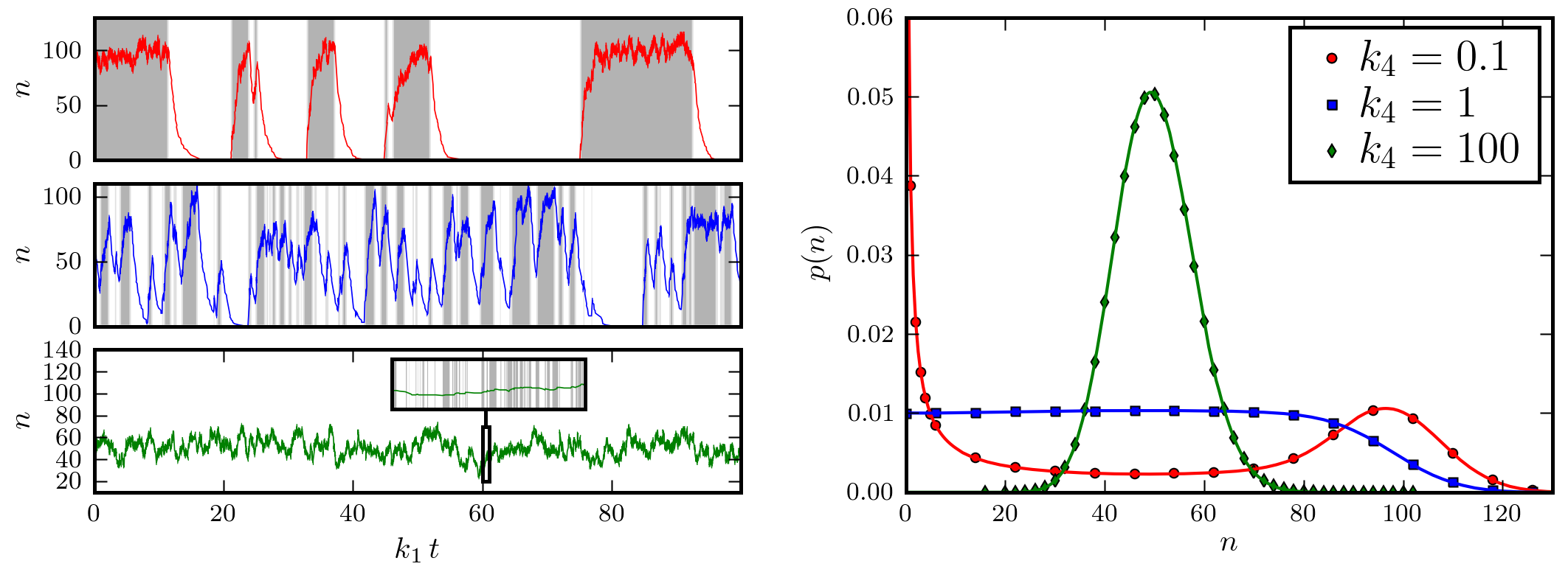
Figure 4: (colour online) Left: Typical trajectories of the system when $k^{\textrm{on}}_{4}=k^{\textrm{off}}_{4}=k_{4}$ is increased (from top to bottom $k_{4}=0.1$, 1 and 100. Other parameters are $k_{1}=1$, $k_{2}=100$ and $k^{\textrm{on}}_{3}=k^{\textrm{off}}_{3}=k_{3}=0.001$. In each panel the grey shading denotes that the switch is on and the line plots the number of enzymes against time. In the third panel the grey shading is only shown in the inset where the trajectory from $k_{1}t=[60,61]$ is detailed. Right: Probability distribution functions of the number of $R_{1}$ molecules in the cell for parameter values corresponding to the trajectories shown in the left panels. The symbols are the result of numerical simulations (see text for details). The full curves plot the analytical results Eqs. (26) and (36) and pass perfectly through the simulation points.

III.1 Analytical solution

Returning to the fully stochastic version of the reaction scheme (1), we now present an exact solution for the steady–state statistics of this model. A solution for the case where $k^{\textrm{off}}_{3}=0$ was sketched in Ref. [35]. Here we present a complete solution for the general case where $k^{\textrm{off}}_{3}\neq 0$, and we discuss the properties of the steady–state as a function of all the parameters of the system.

We first define the probability $p_{s}(n,t)$ that the system has exactly $n$ enzyme molecules at time $t$ and the switch is in the $s$ state (where $s=\{\textrm{on},\textrm{off}\}$). The time evolution of $p_{s}$ is described by the following master equation:

$$\frac{dp_{s}(n)}{dt}=(n+1)k_{1}p_{s}(n+1)+k^{s}_{2}p_{s}(n-1)+nk^{1-s}_{3}p_{1-s}(n)\\ +k^{1-s}_{4}p_{1-s}(n)-(nk_{1}+k^{s}_{2}+nk^{s}_{3}+k^{s}_{4})p_{s}(n)\,\,,$$ (10)

where we use the shorthand notations $\{\textrm{off},\textrm{on}\}\equiv\{0,1\}$, $k^{\textrm{off}}_{2}\equiv 0$ and $k^{\textrm{on}}_{2}\equiv k_{2}$. In the steady state, the time derivative in Eq.(10) vanishes, and the problem reduces to a pair of coupled equations for $p_{\textrm{on}}$ and $p_{\textrm{off}}$:

$$(n+1)k_{1}p_{\textrm{on}}(n+1)+k_{2}p_{\textrm{on}}(n-1)+nk^{\textrm{off}}_{3}p_{\textrm{off}}(n)+k^{\textrm{off}}_{4}p_{\textrm{off}}(n)\\ =(nk_{1}+k_{2}+nk^{\textrm{on}}_{3}+k^{\textrm{on}}_{4})p_{\textrm{on}}(n)\,\,,$$ (11a)

$$(n+1)k_{1}p_{\textrm{off}}(n+1)+nk^{\textrm{on}}_{3}p_{\textrm{on}}(n,t)+k^{\textrm{on}}_{4}p_{\textrm{on}}(n,t)\\ =(nk_{1}+nk^{\textrm{off}}_{3}+k^{\textrm{off}}_{4})p_{\textrm{off}}(n,t)\,\,\,.$$ (11b)

To solve the above equations we introduce the generating functions

$$G_{s}(z)=\sum_{n=0}^{\infty}p_{s}(n)z^{n}\,\,.$$ (12)

The steady-state equations (11) can be now written as a set of linear coupled differential equations for $G_{s}$:

$${\cal L}_{1}G_{\textrm{on}}(z)={\cal L}_{2}G_{\textrm{off}}(z)\,\,,$$ (13a)

$${\cal L}_{3}G_{\textrm{off}}(z)={\cal L}_{4}G_{\textrm{on}}(z)\,\,,$$ (13b)

where ${\cal L}_{i}$ are linear differential operators:

$${\cal L}_{1}(z)= k_{1}(z-1)\partial_{z}-k_{2}(z-1)+k^{\textrm{on}}_{3}z\partial_{z}+k^{\textrm{on}}_{4}\,\,,$$ (14a)

$${\cal L}_{2}(z)= k^{\textrm{off}}_{3}z\partial_{z}+k^{\textrm{off}}_{4}\,\,,$$ (14b)

$${\cal L}_{3}(z)= k_{1}(z-1)\partial_{z}+k^{\textrm{off}}_{3}z\partial_{z}+k^{\textrm{off}}_{4}\,\,,$$ (14c)

$${\cal L}_{4}(z)= k^{\textrm{on}}_{3}z\partial_{z}+k^{\textrm{on}}_{4}\,\,.$$ (14d)

In order to solve the two coupled Eqs. (13) it is first useful to take their difference. After simplification this yields the relation:

$$\partial_{z}G_{\textrm{off}}(z)=-\partial_{z}G_{\textrm{on}}(z)+\frac{k_{2}}{k_{1}}G_{\textrm{on}}(z)\,\,.$$ (15)

Next, we take the first derivative of (13b) and then replace the derivatives of $G_{\textrm{off}}$ with the relation (15). After some algebra, one finds that $G_{\textrm{on}}$ verifies the following second order differential equation:

$$k_{1}(\alpha z-k_{1})G_{\textrm{on}}^{\prime\prime}(z)+(k_{1}\beta-\gamma z)G_{\textrm{on}}^{\prime}(z)-\delta G_{\textrm{on}}(z)=0\,\,,$$ (16)

where the Greek letters are combinations of the parameters of the model:

$$\alpha =k_{1}+k^{\textrm{on}}_{3}+k^{\textrm{off}}_{3}\,\,,$$ (17a)

$$\beta =k_{1}+k_{2}+k^{\textrm{off}}_{3}+k^{\textrm{on}}_{3}+k^{\textrm{off}}_{4}+k^{\textrm{on}}_{4}\,\,,$$ (17b)

$$\gamma =k_{2}(k_{1}+k^{\textrm{off}}_{3})\,\,,$$ (17c)

$$\delta =k_{2}(k_{1}+k^{\textrm{off}}_{3}+k^{\textrm{off}}_{4})\,\,.$$ (17d)

We now introduce the new variable

$$u(z)\equiv u_{z}=\frac{\gamma}{k_{1}\alpha}z-\frac{\gamma}{\alpha^{2}}=u_{0}+z(u_{1}-u_{0})\,\,,$$ (18)

and the new parameter combinations:

$$\zeta=u_{0}+\frac{\beta}{\alpha}\,\,,\qquad\eta=\frac{\delta}{\gamma}\,\,.$$ (19)

We can now write $G_{\textrm{on}}(z)$ (and $G_{\textrm{off}}(z)$) in terms of the variable $u$ (18) by defining the functions

$$J_{s}(u)=G_{s}(z)\;.$$ (20)

The differential equation (16) then reads:

$$uJ_{\textrm{on}}^{\prime\prime}(u)+(\zeta-u)J_{\textrm{on}}^{\prime}(u)-\eta J_{\textrm{on}}(u)=0\,\,.$$ (21)

Looking for a regular power series solution of the form

$$J_{\textrm{on}}(u)=\sum_{n=0}^{\infty}a_{n}u^{n}\,\,,$$ (22)

one obtains the following solution:

$$J_{\textrm{on}}(u)=a_{0}\,{}_{1}F_{1}\left(\eta,\zeta,u\right)\,\,,$$ (23)

where ${}_{1}F_{1}$ denotes the confluent hypergeometric function of the first kind,

$${}_{1}F_{1}\left(\eta,\zeta,u\right)\equiv\sum_{n=0}^{\infty}\frac{(\eta)_{n}}{(\zeta)_{n}}\frac{u^{n}}{n!}$$ (24)

and $(\alpha)_{n}=\alpha(\alpha+1)\dots(\alpha+n-1)$ denotes the Pochhammer symbol.

The constant $a_{0}$ will be determined using the boundary conditions, which we discuss later. We first note that the above result for $J_{\textrm{on}}(u)$ can be translated into $G_{\textrm{on}}(z)$ by replacing $u$ with the expression of $u(z)$ in (22) and expanding in powers of $z$:

$$G_{\textrm{on}}(z)=\sum_{n=0}^{\infty}a_{n}(u_{0}+z(u_{1}-u_{0}))^{n}\\ =\sum_{n=0}^{\infty}a_{n}\sum_{m=0}^{n}u_{0}^{m}[z(u_{1}-u_{0})]^{n-m}\binom{n}{m}\\ =\sum_{n=0}^{\infty}z^{n}\sum_{m=n}^{\infty}a_{m}u_{0}^{m-n}[(u_{1}-u_{0})]^{n}\binom{m}{n}$$ (25)

where we have relabelled the indices $n-m\to n$ and $n\to m$ in the last line. We can identify $p_{\textrm{on}}(n)$ from (12) as the coefficient of $z^{n}$ in the above expression:

$$p_{\textrm{on}}(n)=\sum_{m=n}^{\infty}a_{m}u_{0}^{m-n}(u_{1}-u_{0})^{n}\binom{m}{n}\;.$$ (26)

From (22) and (23) we read off

$$a_{n}=\frac{a_{0}}{n!}\ \frac{(\eta)_{n}}{(\zeta)_{n}}\,.$$ (27)

Substituting (27) in (26) we deduce, using the definition of the hypergeometric function (24) and noting $(\alpha)_{n+m}=(\alpha)_{n}(\alpha+n)_{m}$, that

$$p_{\textrm{on}}(n)=a_{0}\frac{(u_{1}-u_{0})^{n}}{n!}\frac{(\eta)_{n}}{(\zeta)_{n}}\,_{1}F_{1}(\eta+n,\zeta+n,u_{0})\,\,.$$ (28)

In deriving this expression we have, in fact, established the following identity which will prove useful again later:

$${}_{1}F_{1}(\eta,\zeta,u)=\sum_{n=0}^{\infty}\frac{z^{n}(u_{1}-u_{0})^{n}}{n!}\frac{(\eta)_{n}}{(\zeta)_{n}}\,_{1}F_{1}(\eta+n,\zeta+n,u_{0})\,\,.$$ (29)

To compute $G_{\textrm{off}}(z)$, we integrate Eq.(15), which yields, using the form of $J_{\textrm{on}}(u)$ (23):

$$G_{\textrm{off}}(z)+G_{\textrm{on}}(z)\\ -a_{0}\frac{k_{2}(\zeta-1)}{k_{1}(\eta-1)(u_{1}-u_{0})}\,_{1}F_{1}(\eta-1,\zeta-1,u_{z})=\kappa\,\,,$$ (30)

where $\kappa$ is our second integration constant. We then have two constants, $a_{0}$ and $\kappa$, which still need to be determined. The constant $\kappa$ can be found using the normalisation condition $\sum_{n}(p_{\textrm{on}}(n)+p_{\textrm{off}}(n))=1$, which is equivalent to $G_{\textrm{on}}(1)+G_{\textrm{off}}(1)=1$. Using this condition, we obtain

$$\kappa=1-a_{0}\frac{k_{2}(\zeta-1)}{k_{1}(\eta-1)(u_{1}-u_{0})}\,_{1}F_{1}(\eta-1,\zeta-1,u_{1})\,\,.$$ (31)

In order to compute the remaining constant $a_{0}$, we consider the boundary condition at $z=0$. From the definition (12) of the generating function we see that $G_{s}(z=0)=p_{s}(n=0)$. Our boundary condition thus reads:

$$J_{\textrm{on}}(u_{0})+J_{\textrm{off}}(u_{0})=p_{\textrm{on}}(0)+p_{\textrm{off}}(0)\,\,.$$ (32)

Setting $n=0$ in the master equation Eq.(11a) [noting that the term in $p_{\textrm{on}}(n-1)$ vanishes] gives $p_{\textrm{off}}(0)$ in terms of $p_{\textrm{on}}(0)$ and $p_{\textrm{on}}(1)$:

$$p_{\textrm{off}}(0)=\frac{k_{2}+k^{\textrm{on}}_{4}}{k^{\textrm{off}}_{4}}p_{\textrm{on}}(0)-\frac{k_{1}}{k^{\textrm{off}}_{4}}p_{\textrm{on}}(1)\,\,.$$ (33)

Combining Eqs.(30) [with $z=0$] and (31), substituting in Eq.(32), using Eq.(33) to eliminate $p_{\textrm{off}}(0)$, and finally substituting in expressions for $p_{\textrm{on}}(0)$ and $p_{\textrm{on}}(1)$ from Eq.(26), we determine $a_{0}$:

$$a_{0}^{-1}=\left(1+\frac{k_{2}+k^{\textrm{on}}_{4}}{k^{\textrm{off}}_{4}}\right)\,_{1}F_{1}(\eta,\zeta,u_{0})\\ -\frac{k_{1}\eta(u_{1}-u_{0})}{k^{\textrm{off}}_{4}\zeta}\,_{1}F_{1}(\eta+1,\zeta+1,u_{0})\\ -\frac{k_{2}(\zeta-1)}{k_{1}(\eta-1)(u_{1}-u_{0})}\big{[}\,_{1}F_{1}(\eta-1,\zeta-1,u_{0})\\ -\,_{1}F_{1}(\eta-1,\zeta-1,u_{1})\big{]}\,\,.$$ (34)

The final step in obtaining our exact solution is to provide an explicit expression for $p_{\textrm{off}}(n)$. From (30) we have

$$G_{\textrm{off}}(z)=\kappa-G_{\textrm{on}}(z)\\ +a_{0}\frac{k_{2}(\zeta-1)}{k_{1}(\eta-1)(u_{1}-u_{0})}\,_{1}F_{1}(\eta-1,\zeta-1,u_{z})\,\,,$$ (35)

and using the identity (29) we obtain:

$$p_{\textrm{off}}(n)=\kappa\delta_{n,0}+\\ \frac{a_{0}}{n!}\bigg{[}\frac{k_{2}}{k_{1}}(u_{1}-u_{0})^{n-1}\frac{(\eta)_{n-1}}{(\zeta)_{n-1}}\,_{1}F_{1}(\eta+n-1,\zeta+n-1,u_{0})\\ -(u_{1}-u_{0})^{n}\frac{(\eta)_{n}}{(\zeta)_{n}}\,_{1}F_{1}(\eta+n,\zeta+n,u_{0})\bigg{]}\,\,,$$ (36)

where $\delta_{i,j}$ is the Kronecker delta.

Our exact analytical solution (26), (34) and (36) is verified by comparison to computer simulation results in the right panels of Figs. 2 and 4. Here, we plot the probability distribution function for the total number of enzyme molecules:

$$p(n)=p_{\textrm{on}}(n)+p_{\textrm{off}}(n)\;.$$ (37)

Computer simulations of the reaction set (1) were carried out using Gillespie’s stochastic simulation algorithm [38, 39]. Perfect agreement is obtained between the numerical and analytical solutions, as shown in Figs. 2 and 4.

III.2 Properties of the steady–state

Having derived the steady–state solution for $p(n)$, we now analyse its properties as a function of the parameters of the model. We choose to fix our units of time by setting $k_{1}$, the decay rate of enzyme $R$, to be equal to unity (so our time units are $k_{1}^{-1}$). With these units, the plateau value for the number of enzyme molecules in the on switch state is given by $\rho_{\textrm{on}}=k_{2}$. In this section, we will only analyse the case where $\rho_{\textrm{on}}=100$. To further simplify our analysis, we set $k^{\textrm{on}}_{3}=k^{\textrm{off}}_{3}=k_{3}$ and $k^{\textrm{on}}_{4}=k^{\textrm{off}}_{4}=k_{4}$ (a discussion of the case where $k^{\textrm{off}}_{3}=0$ and $k^{\textrm{on}}_{3}\neq 0$ is provided in Ref. [35]). We then analyse the probability distribution $p(n)$ as a function of the $R$-dependent switching rate $k_{3}$ and the $R$-independent switching rate $k_{4}$. The results are shown in the right-hand panels of Fig. 2 and Fig. 4. We consider the three regimes discussed in section II.1: that in which enzyme number fluctuations are much faster than switch flipping, that where the opposite is true, and finally the regime where the two timescales are similar.

In the regime where switch flipping is much slower than enzyme production/decay [$k_{1}\gg\left(k^{\textrm{on}}_{4}+k_{2}k^{\textrm{on}}_{3}/k_{1}\right)$], the probability distribution $p(n)$ is bimodal. This is easily understandable in the context of the typical trajectories shown in the left top panels in Figs. 2 and 4: in this regime, the number of molecules of $R$ always reaches its steady-state value before the next switch flip occurs. It follows then that $p_{\textrm{on}}(n)$ is a bell-shaped distribution peaked around $k_{2}/k_{1}$, while $p_{\textrm{off}}(n)$ is highly peaked around zero, so that the total distribution $p(n)=p_{\textrm{on}}(n)+p_{\textrm{off}}(n)$ is bimodal.

In contrast, when switching occurs much faster than enzyme number fluctuations the probability distribution $p(n)$ is unimodal and bell shaped, as might be expected from the trajectories in the bottom left panels of Figs. 2 and 4. As discussed in section II.1, in this regime the number of $R$ molecules behaves as a standard birth-death process with effective birth rate given by $k_{2}$ multiplied by the average time the switch spends in the on state, and death rate $k_{1}$. For such a birth-death process the steady state probability $p(n)$ is a Poisson distribution with mean given by the ratio of the birth rate to the death rate. To show that our analytical result reduces to this Poisson distribution, we consider the case where enzyme-mediated switching dominates (as in Fig. 2), so that both $k^{\textrm{off}}_{3}$ and $k^{\textrm{on}}_{3}$ are much greater than $k_{1}$. The fraction of time spent in the on state is $k^{\textrm{off}}_{3}/\left(k^{\textrm{on}}_{3}+k^{\textrm{off}}_{3}\right)$, thus the effective birth rate is $k_{2}k^{\textrm{off}}_{3}/\left(k^{\textrm{on}}_{3}+k^{\textrm{off}}_{3}\right)$. In the limit $k^{\textrm{on}}_{3}\to\infty$ and $k^{\textrm{off}}_{3}\to\infty$ with $r=k^{\textrm{off}}_{3}/k^{\textrm{on}}_{3}$ constant, one finds that $\eta\to 1$, $\zeta\to 1$, and $u_{z}\to k_{2}rz/[k_{1}(1+r)]$. Using the fact that $\,{}_{1}F_{1}(1,1,x)=e^{x}$, Eq.(23) gives, in this limit,

$$G_{\textrm{on}}(z)=a_{0}\exp\left(\frac{k_{2}rz}{k_{1}(1+r)}\right)\,\,,$$ (38)

which is the generating function of a Poisson distribution with mean $k_{2}k^{\textrm{off}}_{3}/[k_{1}(k^{\textrm{on}}_{3}+k^{\textrm{off}}_{3})]$. Plugging this result into Eq.(30) and taking again the limit $k_{3}\to\infty$ [and using that $\,{}_{1}F_{1}(0,0,x)=1$] finally yields the result that $p(n)=p_{\textrm{on}}(n)+p_{\textrm{off}}(n)$ is indeed a Poisson distribution. The same approach can be taken for the case of Fig. 4, where $k_{3}$ is constant, and $k^{\textrm{on}}_{4}$ and $k^{\textrm{off}}_{4}$ become very large. The probability distribution $p(n)$ then becomes a Poisson distribution with mean $k_{2}k^{\textrm{off}}_{4}/[k_{1}(k^{\textrm{on}}_{4}+k^{\textrm{off}}_{4})]$. The above result is only valid when $r\neq 0$. In fact, as shown in Fig. 3, when $r=0$ the distribution of $R$ is peaked at 0 and does not have a Poisson-like shape.

Finally, when there is no clear separation of timescales between enzyme number fluctuations and switch flipping, the distribution function for the number of enzyme molecules has a highly non-trivial shape, as shown in the middle panels of Figs. 2 and 4.

IV First passage time distribution

We now calculate the first passage time distribution for our model switch. We define this to be the distribution function for the amount of time that the switch spends in the on or off states before switching. This distribution is biologically relevant, since it may be advantageous for a cell to spend enough time in the on state to synthesise and assemble the components of the “on” phenotype (for example, fimbriae), but not long enough to activate the host immune system, which recognises these components. The calculation for the case $k^{\textrm{off}}_{3}=0$ was sketched in [35]. Here we provide a detailed calculation of the flip time distribution in the more general case $k^{\textrm{off}}_{3}\neq 0$. We find that this dramatically reduces the parameter range over which the flip time distribution has a peak. We demonstrate an important relation between the flip time distributions for the two relevant choices of initial conditions (Switch Change Ensemble and Steady State Ensemble). The first passage time distribution is important and interesting from a statistical physics point of view as it is related to “persistence”. Generally, persistence is expressed as the probability that the local value of a fluctuating field does not change sign up to time $t$ [36]. For the particular case of an Ising model, persistence is the probability that a given spin does not flip up to time $t$. In our model, the switch state $S$ plays the role of the Ising spin. For other problems, there has been much interest in the long-time behaviour of the persistence probability, which can often exhibit a power-law tail. In our case, however, we expect an exponential tail for the distribution of time spent in the on state, because linear feedback will cause the switch to flip back to the off state after some characteristic time. We are therefore interested not only in the tail of the first passage time distribution, but in its shape over the whole time range.

IV.1 Analytical results

We consider the probability $F_{{s}}(T|n_{0}){d}T$ that if we begin monitoring the switch at time $t_{0}$ when there are $n_{0}$ molecules of the flipping enzyme $R$, it remains from time $t_{0}\to t_{0}+T$ in state ${s}$, and subsequently flips in the time interval $t_{0}+T\to t_{0}+T+{d}T$. This probability is averaged over a given ensemble of initial conditions, determined by the experimental protocol for monitoring the switch. Mathematically, the initial condition $n_{0}$ for switch state ${s}$ is selected according to some probability $W_{{s}}(n_{0})$ and we define

$$F_{{s}}(T)=\sum_{n_{0}}F_{{s}}(T|n_{0})W_{{s}}(n_{0})$$ (39)

as the flip time distribution for the ensemble of initial conditions given by $W_{{s}}(n_{0})$.

The most obvious protocol would be to measure the interval $T$ from the moment of switch flipping, so that the times $t_{0}$ correspond to switch flips and the $T$ are the durations of the on or off switch states. We call this the Switch Change Ensemble (SCE). In this ensemble, the probability $W^{\textrm{SCE}}_{s}$ of having $n$ molecules of $R$ at the time $t_{0}$ when the switch flips into the ${s}$ state is:

$$W^{\textrm{SCE}}_{s}(n)=\frac{p_{1-s}(n)(nk^{1-s}_{3}+k^{1-s}_{4})}{\sum_{n}p_{1-s}(n)(nk^{1-s}_{3}+k^{1-s}_{4})}\,\,.$$ (40)

where for notational simplicity, $s=\{1,0\}$ represents $\{{\mathrm{on,off}}\}$. The numerator of the r.h.s of Eq.(40) gives the steady state probability that there are $n$ molecules present in state $1-s$, multiplied by the flip rate into state $s$. The denominator normalises $W^{\textrm{SCE}}_{s}(n)$.

We also consider a second choice of initial condition, which we denote the Steady State Ensemble (SSE). Here, the initial time $t_{0}$ is chosen at random for a cell that is in the ${s}$ state. This choice is motivated by practical considerations: experimentally, it is much easier to pick a cell which is in the ${s}$ state and to measure the time until it flips out of the ${s}$ state, than to measure the entire length of time a single cell spends in the ${s}$ state. The probability $W^{\textrm{SSE}}_{s}$ of having $n$ molecules of $R$ at time $t_{0}$ is then the (normalised) steady-state distribution for the ${s}$ state:

$$W^{\textrm{SSE}}_{s}=\frac{p_{s}(n)}{\sum_{n}p_{s}(n)}\,\,.$$ (41)

To compute the distribution $F(T)$, we first consider the survival probability $h_{s}^{W}(n,t)$, that, given that at time $t=0$ (chosen according to ensemble $W$), the switch was in state ${s}$, at time $t$ it is still in state ${s}$ and has $n$ molecules of enzyme $R$. As the ensemble $W$ only enters through the initial condition, we may drop the superscript $W$ in what follows. The evolution equation for $h_{s}$ is the same as for $p_{s}(n,t)$, but without the terms denoting switch flipping into the $s$ state. This removes the coupling between $p_{\textrm{on}}$ and $p_{\textrm{off}}$ that was present in the evolution equations (11)):

$$\frac{\partial}{\partial t}h_{\textrm{on}}(n,t)=(n+1)k_{1}h_{\textrm{on}}(n+1,t)+k_{2}h_{\textrm{on}}(n-1,t)\\ -(nk_{1}+k_{2}+nk^{\textrm{on}}_{3}+k^{\textrm{on}}_{4})h_{\textrm{on}}(n,t)\,\,\,,$$ (42a)

$$\frac{\partial}{\partial t}h_{\textrm{off}}(n,t)=(n+1)k_{1}h_{\textrm{off}}(n+1,t)-\\ (nk_{1}+nk^{\textrm{off}}_{3}+k^{\textrm{off}}_{4})h_{\textrm{off}}(n,t)\,\,\,.$$ (42b)

Introducing the generating function

$${\tilde{h}}_{s}(z,t)=\sum_{n=0}^{\infty}z^{n}h_{s}(n,t)\;,$$ (43)

the above equations reduce to:

$$\frac{\partial}{\partial t}{\tilde{h}}_{\textrm{on}}(z,t)=(k_{1}-(k_{1}+k^{\textrm{on}}_{3})z)\partial_{z}{\tilde{h}}_{\textrm{on}}(z,t)\\ +(k_{2}z-(k_{2}+k^{\textrm{on}}_{4})){\tilde{h}}_{\textrm{on}}(z,t)\,\,\,,$$ (44a)

$$\frac{\partial}{\partial t}{\tilde{h}}_{\textrm{off}}(z,t)=(k_{1}-(k_{1}+k^{\textrm{off}}_{3})z)\partial_{z}{\tilde{h}}_{\textrm{off}}(z,t)\\ -k^{\textrm{off}}_{4}{\tilde{h}}_{\textrm{off}}(z,t)\,\,\,.$$ (44b)

We can relate $h$ to $F$ by noting that $\sum_{n}h_{s}(n,t)={\tilde{h}}_{s}(1,t)$ is the total probability that the switch has not flipped up to time $t$. Hence,

$$F_{s}(t)=-\partial_{t}{\tilde{h}}_{s}(1,t)\;.$$ (45)

Equations (44) can be solved using the method of characteristics [41]. The result, detailed in Appendix A, is:

$${\tilde{h}}_{\textrm{on}}(z,t)=e^{-\omega_{\textrm{on}}t}e^{k_{2}\tau_{\textrm{on}}(z-k_{1}\tau_{\textrm{on}})(1-e^{-t/\tau_{\textrm{on}}})}\\ \times{\widetilde{W}}(k_{1}\tau_{\textrm{on}}+e^{-t/\tau_{\textrm{on}}}(z-k_{1}\tau_{\textrm{on}}))\,\,\,,$$ (46)

where $\tau_{\textrm{on}}=(k_{1}+k^{\textrm{on}}_{3})^{-1}$ and $\omega_{\textrm{on}}=k^{\textrm{on}}_{4}+k_{2}(1-k_{1}\tau_{\textrm{on}})$. The function ${\widetilde{W}}$ is the generating function for the distribution of enzyme numbers $W(n)$ at the starting time for the measurement:

$${\widetilde{W}}(z)=\sum_{n}W(n)z^{n}\,\,,$$ (47)

where $W$ refers to $W^{\textrm{SCE}}$ or $W^{\textrm{SSE}}$. The function ${\tilde{h}}_{\textrm{off}}(z,t)$ can be obtained in an analogous way: this produces the same expression as for ${\tilde{h}}_{\textrm{on}}$, but with $k_{2}$ set to zero and with all “on” superscripts replaced by “off”:

$${\tilde{h}}_{\textrm{off}}(z,t)=e^{-k^{\textrm{off}}_{4}t}{\widetilde{W}}(k_{1}\tau_{\textrm{off}}+e^{-t/\tau_{\textrm{off}}}(z-k_{1}\tau_{\textrm{off}}))\,\,,$$ (48)

so that $\tau_{\textrm{off}}=(k_{1}+k^{\textrm{off}}_{3})^{-1}$. We can then obtain the distributions $F_{\textrm{on}}(T)$ and $F_{\textrm{off}}(T)$ by differentiating the above expressions, according to Eq.(45):

$$F_{\textrm{on}}(T)=\exp\left(-(\omega_{\textrm{on}}+1/\tau_{\textrm{on}})T+k_{2}\tau_{\textrm{on}}(1-e^{-T/\tau_{\textrm{on}}})\right)\\ \times\Bigg{\{}\Big{[}\omega_{\textrm{on}}e^{T/\tau_{\textrm{on}}}+k_{2}(k_{1}\tau_{\textrm{on}}-1)\Big{]}{\widetilde{W}}\left(k_{1}\tau_{\textrm{on}}+e^{-T/\tau_{\textrm{on}}}(1-k_{1}\tau_{\textrm{on}})\right)\\ +\left(\frac{1}{\tau_{\textrm{on}}}-k_{1}\right){\widetilde{W}}^{\prime}\left(k_{1}\tau_{\textrm{on}}+e^{-T/\tau_{\textrm{on}}}(1-k_{1}\tau_{\textrm{on}})\right)\Bigg{\}}\,\,,$$ (49)

$$F_{\textrm{off}}(T)=\exp\left(-(k^{\textrm{off}}_{4}+1/\tau_{\textrm{off}})T\right)\\ \times\Bigg{\{}k^{\textrm{off}}_{4}e^{T/\tau_{\textrm{off}}}{\widetilde{W}}\left(k_{1}\tau_{\textrm{off}}+e^{-T/\tau_{\textrm{off}}}(1-k_{1}\tau_{\textrm{off}})\right)\\ +\left(\frac{1}{\tau_{\textrm{off}}}-k_{1}\right){\widetilde{W}}^{\prime}\left(k_{1}\tau_{\textrm{off}}+e^{-T/\tau_{\textrm{off}}}(1-k_{1}\tau_{\textrm{off}})\right)\Bigg{\}}\,\,.$$ (50)

In the above expressions, the function ${\widetilde{W}}_{s}$ is given for the steady state ensemble (SSE) by

$${{\widetilde{W}}_{s}}^{\textrm{SSE}}=G_{s}(z)/G_{s}(1)$$ (51)

and for the switch change ensemble (SCE) by

$${{\widetilde{W}}_{s}}^{\textrm{SCE}}(z)=\frac{k^{1-s}_{3}zG^{\prime}_{1-s}(z)+k^{1-s}_{4}G_{1-s}(z)}{k^{1-s}_{3}G^{\prime}_{1-s}(1)+k^{1-s}_{4}G_{1-s}(1)}\,.$$ (52)

IV.2 Relation between SSE and SCE

We now show that a useful and simple relation can be derived between $F_{\textrm{SSE}}(T)$ and $F_{\textrm{SCE}}(T)$. Let us imagine that we pick a random time $t$, chosen uniformly from the total time that the system spends in state ${s}$. The time $t$ will fall into an interval of duration $T$, as illustrated in Fig. 5. We can then split the interval $T$ into the time $T_{1}$ before $t$ and the time $T_{2}$ after $t$, such that $T_{1}+T_{2}=T$.

Figure 5: Schematic illustration of a possible time trajectory for the switch; $t$ is a random time falling in an interval of total length $T$ and splitting it into two other intervals denoted $T_{1}$ and $T_{2}$, as discussed in Section IV.2.

We first note that the probability that our randomly chosen time $t$ falls into an interval of length $T$ is:

$${\textrm{Prob}}(T)\,dT=\frac{T\,F_{s}^{\textrm{SCE}}(T)\,dT}{\int_{0}^{\infty}T^{\prime}\,F_{s}^{\textrm{SCE}}(T^{\prime})\,dT^{\prime}}$$ (53)

Eq.(53) expresses the fact that the probability distribution for a randomly chosen flip time $T$ is $F^{\textrm{SCE}}_{s}(T)\,dT$, but the probability that our random time $t$ falls into a given segment is proportional to the length of that segment. Since the time $T$ is chosen uniformly, the probability distribution for $T_{2}$, for a given $T$, will also be uniform (but must be less than $T$):

$${\textrm{Prob}}(T_{2}|T)\,\,dT=\frac{\Theta(T-T_{2})}{T}\,\,dT\,\,.$$ (54)

One can now obtain $F^{\textrm{SSE}}_{s}$ from ${\textrm{Prob}}(T_{2}|T)$ by integrating Eq.(54) over all possible values of $T$, weighted by the relation (53). This leads to the following relation between $F^{\textrm{SCE}}$ and $F^{\textrm{SSE}}$:

$$F^{\textrm{SSE}}_{s}(T_{2})=\frac{\int_{T_{2}}^{\infty}F^{\textrm{SCE}}_{s}(T^{\prime})\,\,dT^{\prime}}{\int_{0}^{\infty}T^{\prime}F^{\textrm{SCE}}_{s}(T^{\prime})\,\,dT^{\prime}}\,\,.$$ (55)

Taking the derivative with respect to $T_{2}$ this can be recast as

$$\frac{dF^{\textrm{SSE}}_{s}(T)}{dT}=-\frac{F^{\textrm{SCE}}_{s}(T)}{\langle T\rangle_{\rm SCE}}$$ (56)

where $\langle T\rangle_{\rm SCE}$ is simply the mean duration of a period in the on state. We have verified numerically that the expressions (49) and (50) for $F^{\textrm{SSE}}_{s}(T)$ and $F^{\textrm{SCE}}_{s}(T)$ derived above do indeed obey the relation (56). This relation can also be understood in terms of backward evolution equations as we discuss in Appendix B.

IV.3 Presence of a peak in $F(T)$

We now focus on the shape of the flip time distribution $F(T)$, in particular, whether it has a peak. A peak in $F^{\textrm{SCE}}_{\textrm{on}}(T)$ could be biologically advantageous for two complementary reasons. Firstly, after the switch enters the on state there may be some start-up period before the phenotypic characteristics of the on state are established, so it would be wasteful for flipping to occur before the on state of the switch has become effective. Secondly, the on state of the switch may elicit a negative environmental response, such as activation of the host immune system, so that it might be advantageous to avoid spending too long a time in the on state. For example, in the case of the fim switch, a certain amount of time and energy is required to synthesise fimbriae, and this effort will be wasted if the switch flips back into the off state before fimbrial synthesis is complete. On the other hand, too large a population of fimbriated cells would trigger an immune response from the host, therefore the length of time each cell is in the fimbriated state needs to be tightly controlled. We note that for bistable genetic switches and many other rare event processes, waiting time distributions are exponential (on a suitably coarse-grained timescale). This arises from the fact that the alternative stable states are time invariant in such systems. The presence of a peak in $F^{\textrm{SCE}}_{\textrm{on}}(T)$ for our model switch would indicate fundamentally different behaviour, which occurs because the two switch states in our model are time-dependent.

The presence of a peak in the distribution $F(T)$ requires the slope of $F(T)$ at the origin to be positive. Applying this condition to the function $F_{\textrm{on}}$ (49) we get:

$$(k_{2}k^{\textrm{on}}_{3}-(k^{\textrm{on}}_{4})^{2}){\widetilde{W}}(1)-k^{\textrm{on}}_{3}(k_{1}+k^{\textrm{on}}_{3}+2k^{\textrm{on}}_{4}){\widetilde{W}}^{\prime}(1)\\ -(k^{\textrm{on}}_{3})^{2}{\widetilde{W}}^{\prime\prime}(1)>0\,\,.$$ (57)

Eq.(47) allows us to expressing the derivatives of ${\widetilde{W}}(1)$ as functions of the moments of $n$, so that we finally get our condition as a relation between the mean and the variance of the initial ensemble:

$$k_{2}k^{\textrm{on}}_{3}-(k^{\textrm{on}}_{4})^{2}-k^{\textrm{on}}_{3}(k_{1}+2k^{\textrm{on}}_{4})\left\langle n\right\rangle_{W_{\textrm{on}}}\\ -(k^{\textrm{on}}_{3})^{2}\left\langle n^{2}\right\rangle_{W_{\textrm{on}}}>0\,\,,$$ (58)

where $\left\langle\dots\right\rangle_{W_{\textrm{on}}}$ denotes an average taken using the weight $W_{\textrm{on}}$ of Eq. (40) or (41). Analogous conditions can be found for a peak in the off to on waiting time distribution. The moments involved in the above inequality can be computed using the exact results of the previous section. The l.h.s. of (58) can then be computed numerically for different values of the parameters, to determine whether or not a peak is present in $F(T)$.

For the SSE, there is never a peak in the flip time distribution. This follows directly from the relation (56) between the SSE and SCE, which shows that the slope of $F^{\textrm{SSE}}_{s}(T)$ at the origin is always negative:

$$\left.\frac{dF^{\textrm{SSE}}_{s}(T)}{dT}\right|_{T=0}=-\frac{F^{\textrm{SCE}}_{s}(0)}{\left\langle T\right\rangle_{\textrm{SCE}}}<0\,\,.$$ (59)

Thus a peak in the waiting time distribution cannot occur when the initial condition is sampled in the steady state ensemble.

For the SCE, we tested inequality (58) numerically and found that a peak in the distribution $F(T)$ is possible for the time spent in the on state ($F_{\textrm{on}}^{\textrm{SCE}}$), but not for the off to on waiting time distribution ($F_{\textrm{off}}^{\textrm{SCE}}$). This is as expected and can be explained by noting that to produce a peak in $F_{s}^{\textrm{SCE}}(T)$, the flipping rate must increase with time in state $s$. In the on state the flipping rate typically does increase with time as the enzyme $R$ is produced, while in the off state the flipping rate decreases in time as $R$ decays.

An intuitive explanation can be provided for the peak in $F_{\textrm{on}}^{\textrm{SCE}}$. Once the switch enters the on state, the amount of flipping enzyme $R_{1}$ begins to increase, and the on to off flipping rate increases concomitantly. The probability of flipping shortly after entering the on state is thus lower than the probability of flipping later, once more molecules of $R_{1}$ are present. Depending on the parameter values, this may lead to a peak in the distribution $F_{\textrm{on}}^{\textrm{SCE}}$.

The fact that no peak is present in either the SCE ensemble for the off to on flip time distribution $F_{\textrm{off}}(T)$ might be due to the fact that when the switch is in the off state, the amount of flipping enzyme $R_{1}$ and hence the flipping rate decreases after the on to off flip. Therefore, the probability of flipping shortly after the previous flip is higher than the probability of flipping later, when the amount of $R_{1}$ has dropped off, and no peak is expected.

We now discuss the general conditions for the occurrence of a peak in $F_{\textrm{on}}^{\textrm{SCE}}$. We first recall from section III.2 that in the regime where the copy number of the enzyme $R$ relaxes much faster than the switch flips [$k_{1}\gg k^{\textrm{on}}_{4}+k_{2}k^{\textrm{on}}_{3}/k_{1}$], the plateau level of $R$ is reached rapidly after entering the on state, so that the flipping rate out of the on state is essentially constant. This leads to effectively exponentially distributed flip times from the on state, so that no peak is expected. In the opposite regime, where switch flipping is much faster than $R$ number relaxation [$k_{3}\gg 0$], we again expect Poissonian statistics and therefore exponentially distributed flip times. Thus it will be in the intermediate range of $k_{3}$ that a peak in the flip time distribution may occur. The exact condition for this (58) is not particularly transparent as the dependence on the parameters is implicit in the values of the $\left\langle n\right\rangle_{W_{\textrm{on}}}$ and $\left\langle n^{2}\right\rangle_{W_{\textrm{on}}}$. In particular, the effects of the parameters $k_{3}$ and $k_{2}$ are coupled, since the effective $R$-mediated switching rate depends on the copy number of $R$. However we can make a broadbrush description of what is required. First the switch should enter the on state with typical values of $n\ll\rho_{\rm on}$ so that there is an initial rise in the value of $n$ and therefore the flipping rate. Second, we expect that the flipping should be predominantly effected by the enzyme $R$ rather than spontaneously flipping i.e. $k_{3}$ should govern the flipping rather than $k_{4}$.

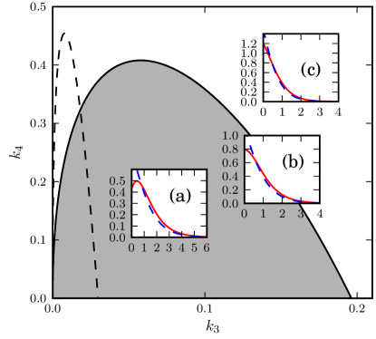
Figure 6: Occurrence of a peak in the waiting time distribution sampled in the Switch Change Ensemble. The shaded area delimits the region where there is a peak (here the parameters are: $k_{1}=1$, $k_{2}=10$ and $k^{\textrm{off}}_{3}=k^{\textrm{on}}_{3}=k_{3}$ and $k^{\textrm{off}}_{4}=k^{\textrm{on}}_{4}=k_{4}$). The dashed line delimits the same region for $k_{2}=100$. The insets show an instance of the distribution both in the SCE (solid red line) and in the SSE (blue dashed line): (a) There is a peak ($k_{2}=10$, $k_{3}=0.1$, $k_{4}=0.1$); (b) On the transition line, where the slope at the origin vanishes ($k_{2}=10$,$k_{3}=0.15$, $k_{4}=0.209384...$); (c) There is no peak ($k_{2}=10$, $k_{3}=0.2$, $k_{4}=0.35$).

Fig. 6 shows the region in the $k_{3}$–$k_{4}$ plane where $F_{\textrm{on}}^{\textrm{SCE}}$ has a peak, for the case where $k^{\textrm{on}}_{3}=k^{\textrm{off}}_{3}=k_{3}$ and $k^{\textrm{on}}_{4}=k^{\textrm{off}}_{4}=k_{4}$. These results are obtained numerically, using the inequality (58). The distribution $F_{\textrm{on}}^{\textrm{SCE}}$ is peaked for parameter values inside the shaded region. The insets show examples of the distributions $F_{\textrm{on}}^{\textrm{SCE}}(T)$ and $F_{\textrm{on}}^{\textrm{SSE}}(T)$ for various parameter values. At the boundary in parameter space between peaked and monotonic distributions (solid line in Fig. 6), $F_{\textrm{on}}^{\textrm{SCE}}(T)$ has zero gradient at $T=0$ (inset (b)). The dashed line in Fig. 6) shows the position of the boundary for a larger value of the enzyme production rate $k_{2}$. As $k_{2}$ increases, the range of values of $k_{3}$ for which there is a peak decreases. Increasing $k_{2}$ increases the number of enzyme present, which will increase both the off to on and on to off switching frequency, since here $k^{\textrm{on}}_{3}=k^{\textrm{off}}_{3}=k_{3}$. Thus it appears that approximately the same qualitative behaviour can be obtained for smaller values of $k_{3}$ when $k_{2}$ is increased.

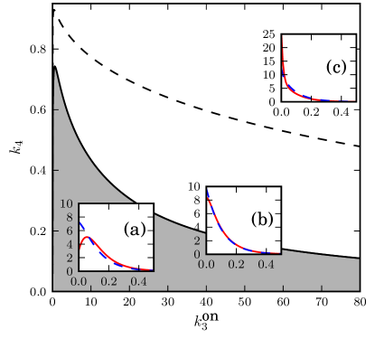
Figure 7: Same plot as Fig. 6 but for $k^{\textrm{off}}_{3}=0$. The shaded area delimits the values of $k_{4}$ and $k^{\textrm{on}}_{3}$ (with $k_{2}=10$) for which there is a peak in the flip time distribution. The dashed line is the separation line for $k_{2}=100$. The examples in the insets have as parameters $k_{2}=10$ and: (a) $k^{\textrm{on}}_{3}=15$, $k_{4}=0.15$; (b) $k^{\textrm{on}}_{3}=50$, $k_{4}=0.162383...$; (c) $k^{\textrm{on}}_{3}=80$, $k_{4}=0.4$.

In our previous paper [35], we analysed the case where $k^{\textrm{off}}_{3}=0$: i.e. the flipping enzyme $R$ switches only in the on to off direction. This case applies to the fim system. Fig. 7 shows the analogous plot, as a function of $k^{\textrm{on}}_{3}$ and $k_{4}$, when $k^{\textrm{off}}_{3}=0$. The region of parameter space where a peak occurs in $F_{\textrm{on}}^{\textrm{SCE}}(T)$ is much wider than for nonzero $k^{\textrm{off}}_{3}$. In this case an increase of $k_{2}$ produces a larger range of parameter values $k^{\textrm{on}}_{3}$ for which there is a peak (dotted line in Fig. 7). Here, the off to on switching process is $R$-independent, and is mediated by $k_{4}$ only (since $k^{\textrm{off}}_{3}=0$). The typical initial amount of $R$ present on entering the on state is thus not much affected by $k_{2}$, although the plateau level of $R$ increases with $k_{2}$. Therefore, as $k_{2}$ increases, the enzyme copy number in the on state becomes more time-dependent, increasing the likelihood of finding a peak.

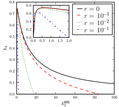
Figure 8: Diagram showing the occurrence of a peak when the ratio $r=k^{\textrm{off}}_{3}/k^{\textrm{on}}_{3}$ is varied. Here $k_{1}=1$ and $k_{2}=10$. The inset shows a zoom of the plot in the vicinity of $k^{\textrm{on}}_{3}=0$.

The comparison between Figs. 6 and 7 suggests that the relative magnitudes of the $R$-mediated switching rates in the on to off and off to on directions, $k^{\textrm{on}}_{3}$ and $k^{\textrm{off}}_{3}$, play a major role in determining the parameter range over which $F_{\textrm{on}}^{\textrm{SCE}}$ is peaked. This observation is confirmed in Fig. 8, where the boundary between peaked and unpeaked distributions is plotted in the $k^{\textrm{on}}_{3}$–$k_{4}$ plane for various ratios $r=k^{\textrm{off}}_{3}/k^{\textrm{on}}_{3}$. The larger the ratio $r$, the smaller the region in parameter space where there is a peak. An intuitive explanation for this might be that as $r$ increases, the the typical initial number of $R$ molecules in the on state increases, so that less time is needed for the $R$ level to reach a steady state, resulting in a weaker time-dependence of the on to off flipping rate and less likelihood of a peak occurring in $F(T)$. If the presence of a peak in $F_{\textrm{on}}^{\textrm{SCE}}$ is indeed an important requirement for such a switch in a biological context, then we would expect that a low value of $k^{\textrm{off}}_{3}$, as is in fact observed for the fim system, would be advantageous.

V Correlations

A peaked distribution of waiting times is by no means the only potentially useful characteristic of this type of switch. In this section, we investigate two other types of behaviour that may have important biological consequences: correlations between successive flips of a single switch, and correlated flips of multiple switches in the same cell. We analyse these novel phenomena using numerical methods. We introduce a new correlation measure which enables us to quantify the extent of the correlation as a function of the parameter space. Our main findings are that a single switch shows time correlations which appear to decay exponentially, and that two switches in the same cell can show correlated or anti–correlated flipping behaviour depending on the values of $k^{\textrm{off}}_{3}$ and $k^{\textrm{on}}_{3}$.

V.1 Correlated flips for a single switch

Biological cells often experience sequences of environmental changes: for example, as a bacterium passes through the human digestive system it will experience a series of changes in acidity and temperature. It is easy to imagine that evolution might select for gene regulatory networks with the potential to “remember” sequences of events. The simple model switch presented here can perform this task, in a very primitive way, because it produces correlated sequences of switch flips: the amount of $R$ enzyme present at the start of a particular period in state ${s}$ depends on the recent history of the system. In contrast, for bistable gene regulatory networks, or other bistable systems, successive flipping events are uncorrelated, as long as the system has enough time to relax to its steady state between flips.

In our recent work [35], we demonstrated that successive switch flips can be correlated for our model switch, and that this correlation depends on the parameter $k^{\textrm{off}}_{3}$: correlation increases as $k^{\textrm{off}}_{3}$ increases. Here, we extend our study and introduce a new measure of these correlations: the two time probability $p(s,t;s^{\prime},t^{\prime})$ that the switch is in position $s$ at time $t$ and in position $s^{\prime}$ at time $t^{\prime}$. In the steady state the two-time probability depends only on the time difference $\tau=t-t^{\prime}$. In order to compare different simulations results, we define the auto-correlation function:

$$C(\tau)=\frac{p_{\textrm{on}-\textrm{on}}(\tau)}{p_{\textrm{on}}}+\frac{p_{\textrm{off}-\textrm{off}}(\tau)}{p_{\textrm{off}}}-1,$$ (60)

where $p_{\textrm{on}-\textrm{on}}(\tau)=p(\textrm{on},t;\textrm{on},t+\tau)$, $p_{\textrm{off}-\textrm{off}}(\tau)=p(\textrm{off},t;\textrm{off},t+\tau)$, and $p_{\textrm{on}}$ ($p_{\textrm{off}}$) is the probability of being in the on (off) state. The correlation function (60) takes values between $-1$ and $1$, in such a way that it is positive for positive correlations, negative for negative correlations and vanishes if the system is uncorrelated. This function allows us to understand whether, given that the switch is in a given position $s$ at time $t$, it will be in the same state $s$ at a later time $t+\tau$.

Fig. 9 shows simulation results for different values of $k^{\textrm{on}}_{3}=k^{\textrm{off}}_{3}=k_{3}$ and $k^{\textrm{on}}_{4}=k^{\textrm{off}}_{4}=k_{4}$. As expected, the correlation function vanishes in the limit of large $\tau$, meaning that in this limit there are no correlations. Furthermore, we can see that the strength of the correlations decreases when either $k_{3}$ or $k_{4}$ are increased. This is consistent with the previous remark that in the limit of large switching rate (i.e. either $k_{3}$ or $k_{4}$) the distribution of enzyme numbers tends to a Poisson distribution. It is thus not surprising that in this same limit the correlations vanish. In the insets of Fig. 9 we plot the same correlation function on a semi-logarithmic scale. The data for the highest values of $k_{3}$ or $k_{4}$ (the dotted green curves) is not shown since the decrease is too sharp, and does not allow for a clear interpretation. For the smallest values of $k_{3}$ and $k_{4}$ (blue curves), the decay seems to be exponential. However, for intermediate values of $k_{3}$ or $k_{4}$ (dashed red curves) the evidence for an exponential decay is less clear and the issue deserves a more extensive numerical investigation. For the sake of completeness we also show in figure 10 similar data for the case where $k^{\textrm{off}}_{3}=0$. We find that qualitatively the data has a very similar behaviour to the case where $k^{\textrm{off}}_{3}=k^{\textrm{on}}_{3}$.

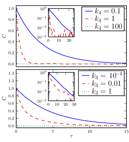
Figure 9: (colour online) The two-time auto-correlation function $C(\tau)$ for $k_{1}=1$, $k_{2}=100$. The insets shows the same data in a semi-log scale. Top: $k_{4}$ is varied with constant $k_{3}=0.001$. Bottom: $k_{3}$ is varied with constant $k_{4}=0.1$.

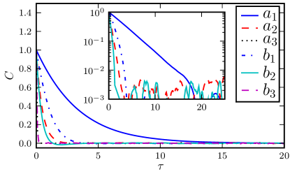
Figure 10: (colour online) The correlation function $C(\tau)$ when $k^{\textrm{off}}_{3}=0$. As previously, $k_{1}=1$ and $k_{2}=100$. The data labelled as $a$ corresponds to $k^{\textrm{on}}_{3}=0.001$ while $b$ corresponds to $k^{\textrm{on}}_{3}=0.01$. For each $a$ and $b$ the superscripts $1$, $2$ and $3$ refer to different values of $k_{4}=0.1$, $1$ and $10$ respectively. The inset shows the same plot on a semi-log scale.

V.2 Multiple coupled switches

Many bacterial genomes contain multiple phase-varying genetic switches, which may demonstrate correlated flipping. For example, in uropathogenic E. coli, the fim and pap switches, which control the production of different types of fimbriae, have been shown to be coupled [42, 43]. Although these two switches operate by different mechanisms, it is also likely that multiple copies of the same switch are often present in a single cell. This may be a consequence of DNA replication before cell division (in fast-growing E. coli cells, division may proceed faster than DNA replication, resulting in up to $\sim 8$ copies per cell). Randomly occurring gene duplication events, which are believed to be an important evolutionary mechanism, might also result in multiple copies of a given switch on the chromosome. It is therefore important to understand how multiple copies of the same switch would be likely to affect each other’s function [44].

Let us suppose that there are two copies of our model switch in the same cell. Each copy contributes to and is influenced by a common pool of molecules of enzyme $R$. Our model is still described by the set of reactions (1), but now the copy number of $S_{\textrm{on}}$ and $S_{\textrm{off}}$ can vary between 0 and 2 (with the constraint that the total number of switches is 2).

To measure correlations between the states of the two switches (denoted $s_{1}$ and $s_{2}$) we define the two switch joint probability $p_{2}(s_{1},t;s_{2},t^{\prime})$ as the probability that switch 1 is in state $s_{1}$ at time $t$ and switch $2$ is in state $s_{2}$ at time $t^{\prime}$. This function is the natural extension of the previously defined two-time probability for a single switch. Thus, in analogy to (60), we can define a two-time correlation function:

$$C_{2}(\tau)=\frac{p_{2}(\textrm{on},t;\textrm{on},t+\tau)}{p_{\textrm{on}}}+\frac{p_{2}(\textrm{off},t;\textrm{off},t+\tau)}{p_{\textrm{off}}}-1\,\,,$$ (61)

where $p_{\textrm{on}}$ ($p_{\textrm{off}}$) is again the steady–state probability for a single switch to be on (off). If the two switches are completely uncorrelated, we expect that $p_{2}(\textrm{on},t;\textrm{on},t^{\prime})=p_{\textrm{on}}^{2}$ and $p_{2}(\textrm{off},t;\textrm{off},t^{\prime})=p_{\textrm{off}}^{2}$, so that $C_{2}(\tau)=0$ (given that $p_{\textrm{on}}+p_{\textrm{off}}=1$). In contrast, if the switches are completely correlated, $p_{2}(\textrm{on},t;\textrm{on},t^{\prime})=p_{\textrm{on}}$, $p_{2}(\textrm{off},t;\textrm{off},t^{\prime})=p_{\textrm{off}}$ and $C_{2}(\tau)=1$. For completely anti-correlated switches, we expect that $p_{2}(\textrm{on},t;\textrm{on},t^{\prime})=p_{2}(\textrm{off},t;\textrm{off},t^{\prime})=0$, and $C_{2}(\tau)=-1$. In Fig. 11 we plot the function $C_{2}(\tau)$ for two identical coupled switches, for several parameter sets. Our results show that for small values of $k_{4}$, there is correlation between the two switches, over a time period $\approx 10k_{1}^{-1}$, which is of the same order as the typical time spent in the on state for these parameter values. Our results also show that the nature of these correlations depends strongly on $k^{\textrm{off}}_{3}$. In the case where $k^{\textrm{off}}_{3}=k^{\textrm{on}}_{3}$ (top panel of Fig. 11), one can see that the correlation is positive, meaning that the two switches are more likely to be in the same state. In contrast, when $k^{\textrm{off}}_{3}$ is set to zero (bottom panel of Fig. 11), the correlation is negative, meaning that the two switches are more likely to be in different states.

To understand these correlations, consider the extreme situation where both the two switches are off, and the number molecules of $R$ has dropped to zero. In this case, the only possible event is a $k_{4}$ mediated switching which could take place, for instance, for the first switch. Then, once the first switch is on, it will start producing more enzyme, and, if $k^{\textrm{off}}_{3}\neq 0$, this will enhance the probability for the second switch to flip on too. This might explain why, when $k^{\textrm{off}}_{3}=k^{\textrm{on}}_{3}$ we see a positive correlation between the two switches. On the other hand, if we consider the opposite situation where both the two switches are on, and the number of molecules of $R$ is around its plateau value, then the on to off switching probability for the two switches will be at its maximum. However, after one of the switches has flipped (e.g. the first), the switching probability will start decreasing, this reducing the flipping rate for the second switch. This suggests that $k^{\textrm{on}}_{3}$ may have the effect of inducing negative correlations, while $k^{\textrm{off}}_{3}$ induces positive correlations. We also point out the presence of a small peak in $C_{2}(\tau)$ in Fig. 11 (indicated by the arrow) which suggests the presence of a time delay: when one switch flips, the other tends to follow a short time later. We leave the detailed properties of these correlations and their parameter dependence to future work.

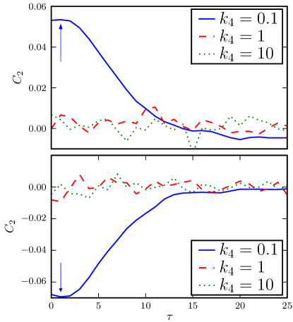
Figure 11: (colour online) Normalised two-time correlation function $C_{2}(\tau)$ for two identical switches. The parameter values are: $k_{1}=1$, $k_{2}=100$,$k^{\textrm{on}}_{3}=0.001$. In the top panel $k^{\textrm{off}}_{3}=k^{\textrm{on}}_{3}$ while in the bottom panel $k^{\textrm{off}}_{3}=0$. The parameter $k_{4}$ is varied from $0.1$ to $100$ in each case.

VI Summary and Outlook

In this paper we have made a detailed study of a generic model of a binary genetic switch with linear feedback. The model system was defined in section II by the system of chemical reactions (1). Linear feedback arises in this switch because the flipping enzyme $R$ is produced only when the switch is in the on state, and the rate of flipping to the off state increases linearly with the amount of $R$. Thus, when the switch is in the on state the system dynamics inexorably leads to a flip to the off state. We have shown that this effect can produce a peaked flip time distribution and a bimodal probability distribution for the copy number of $R$. A mean field description does not reproduce this phenomenology and so a stochastic analysis is required.

We have studied this model analytically, obtaining exact solutions for the steady state distribution of the number of $R$ molecules, as well as for the flip time distributions in the two different measurement ensembles defined in Section IV, the Switch Change Ensemble and the Steady State Ensemble. We have shown how these ensembles are related and demonstrated that the flip time distribution in the Switch Change Ensemble may exhibit a peak but the flip time distribution in the Steady State Ensemble can never do so. We also provide a generic relationship between the flip time distribution sampled in the two different ensembles. Given that in single-cell experiments, measuring the flip time distribution in the SCE is much more demanding than in the SSE, our result provides a way to access the SCE flip time distribution by making measurements only in the SSE. Our flip time calculations are reminiscent of persistence problems in non-equilibrium statistical physics where, for example, one is interested in the time an Ising spin stays in one state before flipping. However, because of the linear feedback of our model switch, the flip time distribution is not expected to have a long tail as in usual persistence problems, rather it is the shape of the peak of the distribution which is of interest.

By studying numerically the time correlations of a single switch, using the two time autocorrelator (60), we have shown that our model switch can play the role of a primitive “memory module”. The two time autocorrelator displays nontrivial behaviour including rather slow decay, which would be worthy of further study. We have also investigated the behaviour of two coupled switches within the same cell, and showed that both positive and negative correlations could be produced by choosing the parameters appropriately. In particular for $k^{\textrm{off}}_{3}=0$, as is the case for the fim switch, anti-correlations were observed, implying that if one switch were on at time $t$, the other would tend to be off at that time and for a subsequent time of about one switch period.

Many open questions and problems remain. At a technical level one would like to compute correlations of a single switch analytically and be able to treat the multiple switch system. The model itself could be refined in several ways, for example, by introducing nonlinear feedback[45, 46]. It has been shown that such feedback allows nontrivial behaviour even at the level of a piecewise deterministic Markov process approximation [46], where one assumes a deterministic evolution for the enzyme concentration, but a stochastic description for the switching. At present our model includes no explicit coupling to the environment, but such coupling could be included in a simple way by adding into the model environmental control of parameters $k_{3}$ or $k_{4}$. To make a closer connection to real biological switches, such as fim, one could extend the model to include, for example, multiple and cooperative binding of the enzymes [26, 27]. One particularly exciting direction, which we plan to pursue in future work, is to develop models for growing populations of switching cells, in which cell growth is coupled to the switch state. Such models could lead to a better understanding of the role of phase variation in allowing cells to survive and proliferate in fluctuating environments.

Appendix A Solution for the survival probability

We show here how to solve Eq.(44a) using the method of characteristics (see e.g. [41]). Introducing the new variable $r(z,t)$, we set

$$\frac{d{\tilde{h}}_{\textrm{on}}(z(r),t(r))}{dr}=\frac{\partial t}{\partial r}\frac{\partial}{\partial t}{\tilde{h}}_{\textrm{on}}(z,t)+\frac{\partial z}{\partial r}\frac{\partial}{\partial z}{\tilde{h}}_{\textrm{on}}(z,t)\\ =\frac{\partial}{\partial t}{\tilde{h}}_{\textrm{on}}(z,t)+\left[k_{1}(z-1)+k^{\textrm{on}}_{3}z\right]\frac{\partial}{\partial z}{\tilde{h}}_{\textrm{on}}(z,t)\,\,.$$ (62)

We can then identify the derivatives of $t$ and $z$ with respect to $r$ as:

$$\frac{dt}{dr}=1\,\,,\qquad\frac{dz}{dr}=k_{1}(z-1)+k^{\textrm{on}}_{3}z\,\,.$$ (63)

Next, we solve these equations for $t(r)$ and $z(r)$ using initial conditions $t(0)=0$ and $z(0)=z_{0}$:

$$t(r)=r\,\,,\qquad z(r)=k_{1}\tau_{\textrm{on}}+e^{r/\tau_{\textrm{on}}}(z_{0}-k_{1}\tau_{\textrm{on}})\,\,,$$ (64)

where $\tau_{\textrm{on}}=(k_{1}+k^{\textrm{on}}_{3})^{-1}$. The reduced ordinary differential equation (ODE) for ${\tilde{h}}_{\textrm{on}}$ is:

$$\frac{d{\tilde{h}}_{\textrm{on}}(r)}{dr}=[k_{2}(z(r)-1)-k^{\textrm{on}}_{4}]{\tilde{h}}_{\textrm{on}}(r)\,\,,$$ (65)

Substituting in the above relation $z(r)$ with its expression given in (64), we get an ordinary differential equation for ${\tilde{h}}_{\textrm{on}}(r)$, which can be solved by separation of variables:

$$\frac{d{\tilde{h}}_{\textrm{on}}}{{\tilde{h}}_{\textrm{on}}}=\tau_{\textrm{on}}(-k_{2}k^{\textrm{on}}_{3}-k^{\textrm{on}}_{4}/\tau_{\textrm{on}}+e^{r/\tau_{\textrm{on}}}k_{2}(z_{0}/\tau_{\textrm{on}}-k_{1}))\,dr\,\,.$$ (66)

Solving the above equation using the initial condition ${\tilde{h}}_{\textrm{on}}(r=0)={\widetilde{W}}(z_{0})$, we arrive at

$${\tilde{h}}_{\textrm{on}}(r)=\exp\bigg{[}-\omega_{\textrm{on}}r+k_{1}k_{2}\tau_{\textrm{on}}^{2}\\ -k_{2}\tau_{\textrm{on}}(e^{r/\tau_{\textrm{on}}}(k_{1}\tau_{\textrm{on}}-z_{0})+z_{0})\bigg{]}{\widetilde{W}}(z_{0})\,\,,$$ (67)

where $\omega_{\textrm{on}}=k^{\textrm{on}}_{4}+k_{2}(1-k_{1}\tau_{\textrm{on}})$. Substituting then from (64) $r\to t$ and $z_{0}\to k_{1}\tau_{\textrm{on}}+e^{-t/\tau_{\textrm{on}}}(z-k_{1}\tau_{\textrm{on}})$ one finally recovers (46).

Appendix B Backwards Evolution Equations for Flip Time Distribution

In this appendix we show how the result (55) can be obtained by considering the backward survival probability:

$$h_{s}^{-}(n_{0},t)=h_{s}(n,0|n_{0},-t)\,\,,$$ (68)

which is the probability that the system has survived in the state $s$ without flipping and with $n$ enzymes at time 0 knowing that it had $n_{0}$ enzyme molecules at a past time $-t$. The probability $h^{-}_{s}$ will verify the backward master equation

$$\frac{\partial}{\partial t}h_{s}^{-}(n_{0},t)=n_{0}k_{1}h_{s}^{-}(n_{0}-1,t)+k_{2}^{s}h_{s}^{-}(n_{0}+1,t)\\ -(n_{0}k_{1}+k^{s}_{2}+n_{0}k_{3}^{s}+k_{4}^{s})h_{s}^{-}(n_{0},t)\,\,.$$ (69)

In section IV we used the forward master equation to compute the flip time distribution in two steps. First, we computed the forward survival probability $h_{s}(n,t)$ with two possible initial conditions, to distinguish the two possible scenarios of measurement. Second, we summed this survival probability over all possible final configurations, and took the time derivative in order to enforce a flipping at the end of the sampling.

An analogous calculation (which we do not detail) can be carried out considering the backward master equation (69), and the final result has to be the same. In fact, we can consider the r.h.s. of (69) as a generator of the backward dynamics. Thus the solution of the backward evolution equation will have as boundary condition the statistics of the final configuration at time 0, and will yield the statistics of the possible corresponding initial configurations at $-t$ (with the additional constraint that the switch never flipped). Since for both SCE and SSE we condition that on switch flips at $t=0$, the boundary condition of (69) has to be taken when the switch is flipping from state $s$ to state $1-s$, and thus corresponds to:

$$h_{s}^{-}(n,0)=W^{\textrm{SCE}}_{1-s}(n)\,\,,$$ (70)

where $W^{\textrm{SCE}}_{s}$ is defined in (40). This is the analogue of the first step described above. The advantage is that now our boundary condition is the same for both the SCE and the SSE.

We can relate $h_{s}^{-}$ to $F_{s}$ by noting that $\sum_{n_{0}}h_{s}^{-}(n_{0},t)$ is the probability that the switch has not flipped going backward for a time $t$. We now have to made a distinction between the SCE and the SSE, since what happens at time $-t$ is precisely the initial ensemble. For the case of the SCE, we want the switch to flip at time $-t$, therefore the flip time distribution is given by:

$$F_{s}^{\textrm{SCE}}(T)=-\partial_{T}\sum_{n_{0}}h^{-}_{s}(n_{0},T)\,\,.$$ (71)

On the other hand, for the case of the SSE, there is no flipping at $-t$ to enforce and the flip time distribution $F_{s}^{\textrm{SSE}}$ is simply proportional to the survival probability:

$$F_{s}^{\textrm{SSE}}(T)=\frac{\sum_{n_{0}}h^{-}_{s}(n_{0},T)}{\int_{0}^{\infty}dT^{\prime}\sum_{n_{0}}h^{-}_{s}(n_{0},T^{\prime})}\,\,.$$ (72)

The denominator in (72) is chosen to ensure normalisation $\int dTF_{s}^{\textrm{SSE}}(T)=1$.

Furthermore, we can compute the average flip time in the SCE using (71):

$$\left\langle T\right\rangle^{\textrm{SCE}}_{s}=\int_{0}^{\infty}dT^{\prime}\,T^{\prime}F^{\textrm{SCE}}(T^{\prime})\\ =\int_{0}^{\infty}dT^{\prime}\sum_{n_{0}}h^{-}_{s}(n_{0},T^{\prime})\,\,,$$ (73)

where an integration by parts has been performed. We can see then that the denominator in Eq.(72) is exactly the average flip time. Finally, integrating Eq.(71) from $T$ to infinity and replacing the result in (73), we obtain

$$F^{\textrm{SSE}}_{s}(T)=\frac{\int_{T}^{\infty}F^{\textrm{SCE}}_{s}(T^{\prime})\,\,dT^{\prime}}{\int_{0}^{\infty}T^{\prime}F^{\textrm{SCE}}_{s}(T^{\prime})\,\,dT^{\prime}}\,\,.$$ (74)

and the result (55) is recovered.

References

- [1] M. W. van der Woude and A. Bäumler, Clin. Microbiol. Reviews 17, 581 (2004).
- [2] I. C. Blomfield, Adv. Microb. Physiol. 45, 3 (2001).
- [3] H. M. Lim and A. van Oudenaarden, Nat. Genetics 39, 269 (2007).
- [4] E. Milo, S. Shen-Orr, S. Itzkovitz, N. Kashtan, D. Chklovskii and U. Alon, Science 298, 824 (2002).
- [5] K. Sneppen and G. Zocchi, Physics in Molecular Biology, Cambridge University Press (2005).
- [6] U. Alon, An Introduction to Systems Biology: Design principles of biological circuits, Chapman and Hall (2007).
- [7] M. B. Elowitz, A. J. Levine, E. D. Siggia and P. S. Swain, Science 297, 1183 (2002).
- [8] P. S. Swain, M. B. Elowitz and E. D. Siggia, Proc. Natl. Acad. Sci. USA 99, 12795 (2002).
- [9] M. Ptashne, A Genetic Switch: Phage and Higher Organisms, 2nd Edition (Blackwell,Cambridge USA, 1992).
- [10] A B Oppenheim, O Kobiler, J Stavans, D L Court and S Adhya, Annu. Rev. Genet. 39 409–29 (2005).
- [11] E. M. Ozbudak, M. Thattai, H. N. Lim, B. I. Shraiman and A. van Oudenaarden, Nature 427, 737 (2004).
- [12] T. S. Gardner, C. R. Cantor and J. J. Collins, Nature 405, 520 (2000).
- [13] J. L. Cherry and F. R. Adler, J. Theor. Biol. 203, 117 (2000).
- [14] F. J. Isaacs, J. Hasty, C. R. Cantor and J. J. Collins, Proc. Natl. Acad. Sci. USA 100, 7714 (2003).
- [15] P. François and V. Hakim, Phys. Rev. E 72,031908 (2005).
- [16] A. D. Keller J. Theor. Biol. 172, 169 (1995).
- [17] A. Lipshtat, A. Loinger, N Q Balaban and O Biham, Phys. Rev. Lett. 96, 188101 (2006).
- [18] M. N. Artyomov, J. Das, M. Kardar and A. K. Chakraborty, Proc. Natl. Acad. Sci. USA 104, 18958 (2007).
- [19] P. B. Warren and P. R. ten Wolde, Phys. Rev. Lett. 92, 128101 (2004).
- [20] P. B. Warren and P. R. ten Wolde, J. Phys. Chem. B 109, 6812 (2005).
- [21] M. J. Morelli, S. Tănase-Nicola, R. J. Allen, and P. R. ten Wolde, Biophys. J. 94, 3413 (2008)
- [22] A. Loinger, A. Lipshtat, N Q Balaban and O Biham, Phys. Rev. E. 75, 021904 (2007).
- [23] E. Aurell and K. Sneppen, Phys. Rev. Lett. 88, 048101 (2002).
- [24] W. Bialek in Advances in Neural Information Processing 13, MIT Press, Cambridge, 2001; cond-mat/0005235.
- [25] T. B. Kepler and T. C. Elston Biophysical J. 81, 3116 (2001).
- [26] D. W. Wolf and A. P. Arkin, OMICS 6, 91 (2002).
- [27] D. Chu and I. C. Blomfield, J. Theor. Biol. 244, 541 (2007).
- [28] D. L. Gally, J. A. Bogan, B. I. Eisenstein and I. C. Blomfield, J. Bacteriol. 175, 6186 (1993).
- [29] H. D. Kulasekara et al., Mol. Microbiol. 31, 1171 (1999).
- [30] S. A. Joyce and C. J. Dorman, Mol. Microbiol. 45, 1107 (2002).
- [31] P. Hinde et al., J. Bacteriol. 187, 8256 (2005).
- [32] D. Low, E. N. Robinson Jr., Z. A. McGee and S. Falkow, Mol. Microbiol. 1, 335 (1987).
- [33] X. W. Nou, B. Braaten, L. Kaltenbach and D. A. Low, EMBO J. 14, 5785 (1995).
- [34] M. Göransson, K. Forsman, P. Nilsson and B. E. Uhlin, Mol. Microbiol. 3, 1557 (1989).
- [35] P. Visco, R. J. Allen, and M. R. Evans, Phys. Rev. Lett. 101 118104 (2008).
- [36] S. N. Majumdar, Current Science 77, 370 (1999).
- [37] B. Derrida, A. J. Bray, C. Godreche J. Phys. A 27, L357-L361 (1994).
- [38] A. B. Bortz et al. ,J. Comput. Phys. 17, 10 (1975).
- [39] D. T. Gillespie, J. Comput. Phys. 22, 403 (1976).
- [40] D. Dubnau and R. Losick, Mol. Microbiol. 61, 564 (2006).
- [41] R. Courant and D. Hilbert, Methods of Mathematical Physics, Volume II, Interscience (1992).
- [42] N. J. Holden and D. L. Gally, J. Med. Microbiol. 53, 585 (2004).
- [43] N. J. Holden, M. Totsika, E. Mahler, A. J. Roe, K. Catherwood, K. Lindner, U. Dobrindt and D. L. Gally, Microbiology 152, 1143 (2006).
- [44] A. S. Ribeiro, Phys. Rev. E 75, 061903 (2007).
- [45] T. Fournier, J.P. Gabriel, C. Mazza, J. Pasquier, J.L. Galbete and N. Mermod, Bioinformatics, 23, 3185 (2007).
- [46] O. Pulkkinen and J. Berg, arXiv:0807.3521.