Accelerated expansion and matter creation

Abstract

A set of cosmological models that takes into account the variation of the particle number is presented. In this context both dark matter and dark energy can be explained using a single component, without assuming any exotic equation of state, solving directly the cosmic coincidence problem.

I Introduction

Currently the observational evidence coming from supernovae studies SNIa , cosmic background radiation fluctuations cmbr , and baryon acoustic oscillations bao , set a strong case for a cosmological (concordance) universe model composed by nearly $70$ percent of a mysterious component called dark energy, responsible for the current accelerated expansion, nearly $25$ percent of dark matter, which populate the galaxies halos and a small percent (around $4$) composed by baryonic matter. The nature of these two dark component remains so far obscure DEDM . In the case of dark matter, we have a set of candidates to be probed with observations and detections in particle accelerators, however the case of dark energy is more elusive. This component not only has to fill the universe at the largest scale homogeneously, and to have the appropriate order of magnitude to be comparable with that of dark matter, but also has to have a negative pressure equation of state, something that was assumed first to explain inflation in the early universe, inspired by high energy theories of particle physics, but which seems to be awkward to appeal for, at these low energy scales. The alternative way used to account for the cosmic acceleration is to consider a modification of general relativity at large scales alterGR . However it seems to be a difficult route to follow, considering the subtleties in the interpretation of the observations even in the simplest model based on general relativity.

To describe the universe at the largest scale, as is the case in cosmology, we have to make certain assumptions regarding the local distribution of matter and its characteristics. As is well known (and explained in several classic books tolman , weinberg , peebles ) the energy-momentum tensor used in the Einstein’s equations is imported from considerations made in special relativity, through a covariant generalization supported by the equivalence principle. The assumption about homogeneity and isotropy leads to consider the matter content of the universe as a fluid. In the case of a perfect fluid, defined as a mechanical medium incapable of exerting transverse stresses, it takes the standard diagonal form

$$T^{\mu\nu}=(\rho+p)U^{\mu}U^{\nu}-g^{\mu\nu}p,$$ (1)

where $\rho$ is identified as the energy density of the fluid, $p$ is the proper hydrostatic pressure, $U^{\mu}=dx^{\mu}/ds$ are the components of the macroscopic velocity of the fluid with respect to the actual coordinate system and $g^{\mu\nu}$ is the metric of it. The expression (1) is what is measured by an observer at rest in the fluid, who examines an element of the fluid small enough so that gravitational curvature can be neglected. The conclusion of applying the energy conservation relation to this tensor

$$T^{\mu\nu}_{\hskip 8.5359pt;\nu}=0,$$ (2)

is that perfect fluids behave adiabatically when examined by a local observer, satisfying the equation

$$d(\rho V)+pdV=0,$$ (3)

where $V$ is the physical volume of the region considered. Is usual to take as the volume $V=d_{f}^{3}$, where $d_{f}$ is a physical distance of the order of the region we are interested in. Using that $d_{f}=d_{c}R(t)$, leads to the well know result

$$\dot{\rho}+3\frac{\dot{R}}{R}(\rho+p)=0,$$ (4)

To get this result, it was assumed also that particle number is conserved $N^{\mu}_{;\mu}=0$, where $N^{\mu}=nU^{\mu}$ with $n$ the particle number density.

A way to modify (3) without spoiling adiabatic evolution is by adding a work term due to the change of the particle number $N$. In prigogine , the authors studied this case as an alternative cosmological model, considering the change of the particle number, assuming that such a correction have to be considered during matter creation. This work actually suggested for the first time, a way to incorporate the particle creation process in the context of cosmology, in a self consistent way. In fact, the original claim made by Zeldovich zeldov70 , that gravitational particle production can be described phenomenologically by a negative pressure, is realize here in a beautiful way. A covariant formulation of the model was presented in CLW90 .

The context where these considerations would be important were mentioned to be; the steady-state cosmological model, the warm inflationary scenario and within the standard inflationary scenario, during the reheating phase. Based on this work, the studies of cosmological models with matter creation lima96 were initiated, which were rapidly recognized as be potentially important to explain dark energy harko . In particular, in Ref.zsbp01 the authors established a model where dark energy can be mimicked by self-interactions of the dark matter substratum. Within the same framework, models of interacting dark energy and dark matter were proposed interact . Actually, in these studies is possible to have consistently, a universe where matter creation proceeds within an adiabatic evolution. More recently, Lima et al.,lima08 have presented a study of a flat cosmological model where a transition from decelerated to accelerated phase exist. They explicitly show that previous models considered lima99 , does not exhibit the transition, and study the observational constraints on the model parameters.

In this work I consider non flat models where by modifying the first law, enable us to explain the current acceleration of the universe expansion through a fictitious pressure component coming from changes in the total particle number. In this way, the dark energy component is basically an effect due to the dark matter creation process in the universe, fact that enable us to explain easily the cosmic coincidence problem; it is not strange to have a similar contribution from these two component, because they are just one component; dark matter. I also demonstrate that a non constant matter creation rate can indeed lead to a transition from a decelerated to an accelerated regime even in the case of non flat geometries. In the next section I derive the equations of motion in the case of matter creation. Then, I open section III with a very simple model with a non constant creation rate, that resemble the $\Lambda$CDM model. After this, I discussed the case of the transition from a decelerated to an accelerated expansion in non flat models.

II Matter creation

The incorporation of the variable $N$ into the cosmological scenario, modifies the first law as

$$d(\rho V)+pdV-(h/n)d(nV)=0,$$ (5)

where $h$ is the enthalpy (per unit volume), $n=N/V$ is the number density and $\rho$ is the energy density. The important thing to stress here is that the universe evolution continues to be adiabatic, in the sense that the entropy per particle remains unchanged ($\dot{\sigma}=0$). The extra contribution can be interpreted as a non thermal pressure defined as

$$p_{c}=-\frac{h}{n}\frac{d(nV)}{dV}.$$ (6)

This is the source that produces the current acceleration of the universe expansion. Once the particle number increases with the volume ($dN/dV>0$), we obtain a negative pressure.

Now, because we are considering matter creation, we have to impose the second law constraint as

$$dS=\frac{s}{n}d(nV)\geq 0,$$ (7)

where $s=S/V$ is the entropy density. From (5) we find that the new set of Einstein equations are

$$H^{2}+\frac{k}{R^{2}}=\frac{8\pi G}{3}\rho$$ (8)

$$\dot{\rho}=\frac{\dot{n}}{n}(\rho+p)$$ (9)

and from (7) we have to supply an extra relation between $n$ and the Hubble parameter

$$\dot{n}+3Hn=3H\beta,$$ (10)

where $\beta$ is a definite positive function. The set of equations (8), (9) and (10) completely specified the system evolution. The standard adiabatic evolution is easily recovered: setting $\beta=0$ implies that $\dot{n}/n=-3H$, which leads to the usual conservation equation from (9). It is interesting to note that Eq.(9) enable us to determine the pressure; for example if $\rho=mn$ Eq.(9) implies $p=0$, and furthermore if $\rho=aT^{4}$ and $n=bT^{3}$ implies $p=\rho/3$.

III Models

Let us assume first here that

$$\frac{dN}{dV}=\beta_{0}$$ (11)

The arguments in favor of this hypothesis would be given in short. Let us study here its consequences. If we consider $V=R^{3}$, relation (11) leads to $\beta=\beta_{0}$. From (10) we finds the solution for the density number to be

$$n(t)=\beta_{0}+\frac{C_{1}}{R(t)^{3}},$$ (12)

where $C_{1}$ is a constant of integration. Assuming $\rho=mn$ as for non-relativistic matter (that leads to que usual equation of state $p=0$ as we discussed that at the end of the last section), we get for the energy density

$$\rho(R)=m\beta_{0}+\frac{mC_{1}}{R^{3}},$$ (13)

that resembles the combined contribution of a cosmological constant and dust. The level of fine tuning here to obtain an accelerated expansion is relatively smaller than in the usual $\Lambda$CDM model, because in this case, both terms come from the same function, and we know that we can obtain an accelerated expansion phase after some time from (8). Note however that the equation of state has not been modified, $\rho$ is still the non-relativistic contribution. We do not have to introduce any exotic component - with a negative pressure - to describe the current expansion acceleration. Given the current status of the dark matter and dark energy problem DEDM , we can use this idea as a possible way to understand it.

In terms of the exotic dark energy fluid with energy density $\rho_{X}$ and pressure $p_{X}$, the solution (13) can be expressed as

$$\rho_{X}=m\beta,\hskip 28.45274ptp_{X}=\omega\rho_{X},$$ (14)

where now there must be two copies of Eq.(9) with the one corresponding to dark energy being

$$\dot{\rho_{X}}=\frac{\dot{n}}{n}(\rho_{X}+p_{X}),$$ (15)

and $n$ stand only for the second term in Eq. (13). Of course, from Eqs. (8), (13) and (15) we get $\omega=-1$; e. i., the ansatz (11) has leads us to the case of a purely cosmological constant contribution. In general, we can always separate the contribution for “purely” non-relativistic matter $\rho_{m}$ $(\propto R^{-3}$) from the dark energy. In this case $\rho=\rho_{m}+\rho_{X}$, and the pressure can be written as

$$p_{X}=-m\beta_{0}.$$ (16)

We can notice that $p_{X}$ is exactly the non thermal pressure computed in (6) (recall that $p_{m}=0$).

I have to stress here that the main result derived in this section means that we have a single contribution, which satisfy the non-relativistic matter equation of state, that describe both dark matter and dark energy simultaneously, and in this way solving automatically the coincidence problem. This dark unification mechanism does not have the problem studied in STZW , because in the cases studied in that paper, for example the Chaplygin gas model chaplygin , the sound velocity of the dark matter is not zero, leading to instabilities. That happens because the Chaplygin gas interpolates between the equation of states for dark matter and dark energy. This does not happens here, because there is just one equation of state; that of non-relativistic matter.

IV Decelerated/accelerated transition

As is well known from observations of supernovae, a transition from a decelerated to an accelerated expansion occurs in the recent history of the universe. Depending on what is used to model dark energy, different redshift have been obtained between $0.5$ to $1$.

This topics was recently discussed in lima08 where the authors specialized in a flat cosmology, where a explicit transition can be achieved from a decelerated to an accelerated expansion. In this section we generalize this work to non flat universes, by using a model (see equation (10)) with

$$\beta=n\gamma\frac{H_{0}}{H}$$ (17)

where $\gamma$ is a constant parameter (is exactly the same letter introduced in lima08 ). In what follows, a non relativistic matter equation of state is assumed ($p=0$).

Introducing (17) in (10) leads to the following solution

$$n(R)=n_{0}\left(\frac{R_{0}}{R}\right)^{3}e^{3H_{0}\gamma(t-t_{0})}.$$ (18)

Is evident the meaning of the subscript zero. Because $\rho=mn$ for non-relativistic matter, the Friedman equation can be written as

$$\dot{R}^{2}R+kR=\kappa e^{3H_{0}\gamma(t-t_{0})},$$ (19)

where $\kappa=8\pi G\rho_{0}R_{0}^{3}/3$. Evaluating this expression for the reference time $t=t_{0}$ we obtain that

$$k=H_{0}^{2}R_{0}^{2}(\Omega_{0}-1),$$ (20)

where we have defined $\Omega_{0}=\rho/\rho_{c}$, with $\rho_{c}=3H_{0}^{2}/8\pi G$ being the critical energy density. Using this in (19) we obtain

$$\frac{\dot{R}^{2}}{R_{0}^{2}}=H_{0}^{2}\left[1-\Omega_{0}+\Omega_{0}\left(\frac{R_{0}}{R}\right)e^{3H_{0}\gamma(t-t_{0})}\right].$$ (21)

Clearly, for $\gamma=0$ this expression reduces to the standard result.

In order to compare with observations, we shall compute the deceleration parameter, $q=-R\ddot{R}/\dot{R}^{2}$, in terms of the redshift. By differentiating (21) respect to cosmic time we find

$$q=-\frac{(3H_{0}\gamma-H)e^{3H_{0}\gamma(t-t_{0})}}{2H\left[1-\Omega_{0}+\Omega_{0}(\frac{R_{0}}{R})e^{3H_{0}\gamma(t-t_{0})}\right]}.$$ (22)

So, from (21) we find the scale factor in term of the cosmic time, $R(t)$, and using that $R=R_{0}(1+z)^{-1}$, we can use (22) to write down $q(z)$. As an example, for $\Omega_{0}=1.2$ and $\gamma=0.4$ the deceleration parameter computed from (22) in terms of the redshift is shown in Figure 1.

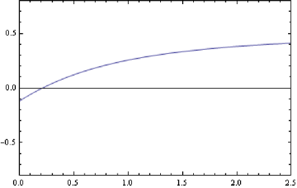
Figure 1: $q(z)$ versus $z$. An example of Eq.(22) in terms of the redshift $z$. In this case $\Omega_{0}=1.2$ and $\gamma=0.4$. See the text for comments.

For a fixed $\Omega_{0}$, a crossing redshift exist if $\gamma>1/3$. Otherwise, the universe never made the transition. For $\Omega_{0}<1$, the situation is qualitatively similar, in this case with a smaller slope.

In the case of a flat universe, $\Omega_{0}=1$ we obtain

$$q_{0}=\frac{1}{2}(1-3\gamma\frac{H_{0}}{H}),$$ (23)

which coincides with the result obtained in lima08 .

To complete the analysis, I will briefly discuss the case of the interaction term $\Gamma=3\beta H$, discussed also in lima96 . In this case, the deceleration parameter can be explicitly written in terms of the redshift as

$$q(z)=\left(\frac{1-3\beta}{2}\right)\left(\frac{\Omega_{0}(1+z)^{1-3\beta}}{\Omega_{0}(1+z)^{1-3\beta}+1-\Omega_{0}}\right).$$ (24)

If we specialize to a flat universe, $\Omega_{0}=1$, $q$ becomes a constant, showing no transition between decelerated to an accelerated regime. However, the non flat case, is not different. Actually, the $z$ dependence make the values of $q$ to vary with redshift, but there is no redshift for which $q=0$.

So the challenge would be to estimate the function $dN/dV$ enabling us to give the best fit to the observations. The first model considered in the last section shows us a very simple scenery to follow. Let me proceed further and complicate a little bit the model setup. For example, we can study the case of a distribution of matter which is oscillatory with volume. It means that instead of consider (11), we use $dN/dV=\beta\cos(V/V_{c})$. This implies that matter distribution is characterized by a volume $V_{c}$. In this case, the energy density behaves as $\rho=C_{1}/R^{3}+(\beta V_{c}/R^{3})\sin(R^{3}/V_{c})$, so when the volume considered is small enough $R^{3}\ll V_{c}$, this solution approaches (13). A typical profile of the scale factor evolution is shown in Fig. 2.

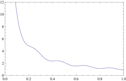
Figure 2: Typical profile of the scale factor evolution in the case of a oscillatory distribution of matter. Although the global behavior is $\propto R^{-3}$, the oscillatory nature of the distribution of matter produces wiggles that can be associated to short periods of accelerated expansions. The scales are arbitrary.

In this letter I have demonstrated that considering small changes in the total number of particles in our universe, offer a possible way to understand the current accelerated expansion measurements, without using any exotic energy component. Also, this scenario explain also the cosmic coincidence problem, basically showing that these two components, dark matter and dark energy, are the of the same nature, but their act at different scales. This way of understand the SNIa observations, implies that cosmology have a new window to explore the universe considering matter creation, encoded in the function $dN/dV$. Although I have discussed some examples for this function, neither has been obtained from a fundamental theoretical basis.

References

- (1) A. Riess et al., Astrophys. J. 607, 665 (2004); J.L. Tonry et al., Astrophys. J. 594, 1 (2003).
- (2) D.J. Eisenstein et al., Astrophys. J. 633, 560 (2005).
- (3) D.N. Spergel et al., Astrophys. J. Suppl. 170, 377 (2007).
- (4) J.A. Frieman, M.S. Turner and D. Huterer, arXiv: astro-ph/0803.0982; M. Taoso, G. Bertone and A. Masiero, arXiv: astro-ph/0711.4996; D. Hooper and E.A. Baltz, Annu. Rev. Nucl. Part. Sci. 58, (2008)(arXiv: hep-ph/0802.0702).
- (5) S.M. Carroll, V. Duvvuri, M. Trodden and M. Turner, Phys. Rev. D 70, 043528 (2004); S. Capozziello, “Dark energy and dark matter as curvature effects”, to be published in the Proceedings of the 11th Marcel Grossmann Meetng, Berlin, July (2006).
- (6) R.C. Tolman, Relativity, Thermodynamics and Cosmology, Oxford (1935).
- (7) S. Weinberg, Principles of Gravitation and Cosmology, New York, Wiley (1972).
- (8) P.J.E. Peebles, Principles of Physical Cosmology, Princeton, Princeton University Press (1993).
- (9) I. Prigogine, J. Geheniau, E. Gunzig and P. Nardone, Proc. Natl. Acad. Sci. USA, Vol 85, 7428 (1988); ibid, Gen. Rel. Grav. 21, 767 (1989).
- (10) Ya. B. Zeldovich, JETP Lett. 12, 307 (1970).
- (11) J.A. Lima, M.O. Calvao and I. Waga, Frontier Physics, Essays in Honor of Jayme Tiomno, World Scientific, 1991, arXiv: astro-ph/0708.3397.
- (12) L.R.W. Abramo and J.A.S. Lima, Class. Quant. Grav. 13, 2953 (1996); W. Zimdahl, Phys. Rev. D 53, 5483 (1996); W. Zimdahl and D. Pavón, Mon. Not. R. Astron. Soc. 266, 872 (1994).
- (13) W. Zimdahl, Phys. Rev. D 61, 083511 (2000); M.K. Mak and T. Harko, Aust. J. Phys. 52, 659 (1999).
- (14) W. Zimdahl, D.J. Schwarz, A.B. Balakin and D. Pavon, Phys. Rev. D 64, 063501 (2001).
- (15) L. Amendola, S. Tsujikawa and M. Sami, Phys. Lett. B 632, 155 (2006); L. Amendola and C. Quercellini, Phys. Rev. D 68, 023514 (2003); L.P.Chimento, A.S. Jakubi, D. Pavon and W. Zimdahl, Phys. Rev. D 67, 083513 (2003); W. Zimdahl and D. Pavon, Phys. Lett. B 521, 133 (2001); L. Amendola, Phys. Rev. D 62, 043511 (2000).
- (16) J.A.S. Lima, F.E. Silva and R.C. Santos, Class. Quant. Grav. 25, 205006 (2008).
- (17) J.A.S. Lima and J.S. Alcaniz, Astron. Astrophys. 348, 1 (1999); J.S. Alcaniz and J.A.S. Lima, Astron. Astrophys. 349, 729 (1999).
- (18) H.B. Sandvik, M. Tegmark, M. Zaldarriaga and I. Waga, Phys. Rev. D 69, 123524 (2004); R. Bean and O. Dore, Phys. Rev. D 68, 023515 (2003).
- (19) A. Kamenshchik, U. Moschella and V. Pasquier, Phys. Lett. B 511, 265 (2001); M.C. Bento, O. Bertolami, A.A. Sen, Phys. Rev. D 67, 063003 (2003).