Epidemics with Multistrain Interactions: The Interplay Between Cross Immunity and Antibody-Dependent Enhancement

Abstract

This paper examines the interplay of the effect of cross immunity and antibody-dependent enhancement (ADE) in mutistrain diseases. Motivated by dengue fever, we study a model for the spreading of epidemics in a population with multistrain interactions mediated by both partial temporary cross immunity and ADE. Although ADE models have previously been observed to cause chaotic outbreaks, we show analytically that weak cross immunity has a stabilizing effect on the system. That is, the onset of disease fluctuations requires a larger value of ADE with small cross immunity than without. However, strong cross immunity is shown numerically to cause oscillations and chaotic outbreaks even for low values of ADE.

The spreading of infectious diseases having multiple strains in a population can exhibit very complex dynamics, ranging from periodic and quasi-periodic outbreaks to high dimensional chaotic behavior. Several sociological and epidemiological factors characterize the disease spread at different levels, such as interactions among the disease strains, social contacts, and human immune responses. In this work we focus on dengue fever, a vector born disease which has exhibited as many as 4 different strains, and is endemic in large areas of Southeast Asia, Africa and the Americas. A notable feature of dengue is its interaction with the human immune system. When an individual is infected with dengue, the immune system triggers an antibody response which will temporarily protect against secondary infections. However, when the level of protection decreases, secondary infections may be possible and the presence of low level antibodies triggers an increase in the infectiousness of the individual. This effect is called antibody-dependent enhancement (ADE). In this paper we study a mathematical model for the spreading of dengue fever. While ADE alone is proved to trigger large amplitude chaotic oscillations, we show that including weak temporary cross immunity stabilizes the system. In contrast, we also show that strong cross immunity destabilizes the dynamics. These results will help understand implementation of proper control strategies when using future vaccines.

I Introduction

Understanding the dynamics of multistrain diseases is a key topic in population biology. A suitable model class for such diseases, which include influenza, malaria and dengue (Hal07, ), must take into account the possibility of interactions among the serotypes or strains. The nature of multistrain interactions strongly affects the impact of the disease on the population as well as the mechanisms for its control.

One prominent example of an endemic multistrain disease is that of dengue and dengue hemorrhagic fever (DHF). Located in Africa, the Americas, and Southeast Asia, dengue is one of several emerging tropical diseases (Gubler_MB, ). There is no vaccine, although clinical trials are underway in order to generate an immune response across all strains (GuyA08, ). Approximately 2.5 billion people are at risk for contracting dengue (B:who1, ; B:who2, ), and between 50 and 100 million cases are reported each year (Gubler_MB, ). The dominant four dengue viruses have progressively spread geographically to virtually all tropical countries to create a global pandemic resulting in several hundred thousand hospitalizations every year (Halstead, ). Since dengue is so far reaching and endemic, it is important to understand how it fluctuates in time, so that when proper vaccines are developed, implementation may be guided by a more thorough understanding of the disease. Dengue is known to exhibit as many as four coexisting serotypes (strains) in a region such as Thailand. Dengue displays a distinctive mechanism of interaction among the strains, called antibody-dependent enhancement. Once a person is infected and recovers from one serotype, life-long immunity to that serotype is conferred. Antibodies are developed specifically for the first challenging serotype and not the other serotypes. In the presence of a new secondary infection, low level antibodies developed from the first infection form complexes with the second challenging serotype so that the virus can enter more cells, increasing viral production (B:CDC, ). Viral loads are associated with transmissibility, and it is hypothesized that individuals with secondary infection are more infectious than during their first infection. This increased transmission rate in subsequent infections is known as antibody-dependent enhancement (ADE). In vitro studies of dengue fever suggested that the ADE phenomenon may be due to the increasing of the infection of cells bearing the IgG receptor (G-immunoglobulin) (HalOro77, ).

The impact of ADE on the modeling of multistrain diseases such as dengue is quite profound (FerAndGup99, ). In general, the first models were of SIR type, with ADE included, and they showed that for sufficiently high ADE, oscillations were possible. In contrast, single strain SIR models only have isolated equilibria and cannot show fluctuations without external seasonal drives or noise. Recent work has begun to analyze in detail the effect of ADE quantitatively on the dynamics (LeahPRE, ; LeahJMB, ), as well as the competition between serotypes (LeahPNAS, ). It is also still unclear if ADE increases transmission of the disease or increases mortality, shortening the effective infectious period. Theoretical studies suggested that the former case allows for coexistence of strains with periodic and chaotic disease outbreaks (LeahPNAS, ), while in the latter the phenomenon may decrease persistence (KawEtAl03, ). Throughout this work we shall assume the first case to hold.

In addition to ADE, another type of interaction between the strains occurs. Recently, cross protection, or cross immunity between serotypes, has been conjectured to play a role in the dynamics of dengue (NagaoK08, ; AdamsHZMNKB06, ). While a primary dengue infection with a particular serotype may confer long-life immunity to that strain (Sab52, ; Inn97, ), it may also confer temporary cross immunity to the other serotypes. Cross immunity may act like a prophylactic to different strains and may also possess different efficacies. That is, cross immunity may be total (i.e., a period of cross immunity always occurs in the event of a primary infection), or partial (i.e., only a fraction of the actual infected population becomes cross immune before being susceptible again to the disease). In general, the length of the cross immunity period may vary depending on the disease. Cross immunity may result from an immunological response to the disease. It acts to reduce the susceptibility to a secondary infection, lowering the effective probability for reinfection to happen (AdaBoo06, ). In the case of dengue fever, cross immunity may last from two up to nine months (WeaRoh06, ), after which the antibodies have dropped to sufficiently low levels that allow infection with other strains and subsequent ADE. Cross immunity plays a crucial role in the co-circulation of strains (AdaSas07, ; NunEtAl05, ) and the pathogen diversity (AbuFer04, ; KawEtAl03, ).

Several studies involving separately cross immunity (EstVar03, ; AndLinLev97, ; AbuFer04, ; GupEtAl98, ) and ADE (FerAndGup99, ; LeahPNAS, ; LeahPRE, ; LeahJTB, ) have been published in the past. The presence of both ADE and cross immunity in such models has not been extensively studied, although some recent models have begun to address this interaction. As an example of such a model, Ref. AguSto07 studied the impact of ADE on the dynamics of a multistrain disease with temporary cross immunity, giving particular importance to the “inverse ADE” hypothesis (i.e., reduced infectivity of secondary infections). Ref. AdaBoo06 considered different types of ADE while allowing for lifelong partial cross immunity. Ref. WeaRoh06 showed that including both ADE and temporary cross immunity is necessary to produce periodicities consistent with epidemiological data. Finally, Ref. NagaoK08 included different mechanisms of cross immunity in a model with ADE in order to test the impact of a period of cross protection on the incidence of secondary dengue cases. They found that including clinical cross immunity, in which a challenge with a previously unexperienced serotype results in an increase of immunity towards the challenging serotype, gives incidence patterns of secondary dengue infections that are compatible with collected data.

The aim of our work is to study in detail the impact of both ADE and temporary, partial cross immunity on the dynamics of the mutistrain diseases. The outline of the paper is as follows: In Section II we introduce the model, in Section III we analyze the effect of weak cross immunity on the system, in Section IV we restrict ourselves to the case of no ADE to investigate the impact of strong cross immunity on the dynamics, and in Section V we include also ADE and study the interplay between cross immunity and ADE. Section VI concludes with a summary and discussion.

II Description of the model

The dynamical system considered in this paper is based on the SIR (Susceptible - Infected - Recovered) model and is a generalization of a multistrain model with ADE studied previously (LeahPRE, ; LeahJTB, ). We write the model for an arbitrary number $n$ of serotypes, and we include both ADE and cross immunity in the dynamics. A set of ordinary differential equations describes the rate of change of the population in each of the classes. We assume the population size to be normalized to unity, so each state represents a fraction of the total population. The quantities that enter the equations are the fraction of susceptibles to all serotypes, denoted by $s$; the primary infectives with strain $i$, $x_{i}$; the cross immunes that are recovered from strain $i$ and have temporary cross immunity to all strains, $c_{i}$; the recovereds from strain $i$ that are immune to strain $i$ only, $r_{i}$; and the secondary infectives with strain $j$ previously infected with strain $i\neq j$, $x_{ij}$. The flow of an individual through the population in the two strain case is shown in Figure 1. Tertiary infections are not included (B:Nisalak, ), so all individuals enter the completely immune class $r_{tot}$ after recovery from a secondary infection. The dynamical system is as follows:

$$\frac{ds}{dt} = \mu-\beta s\sum_{i=1}^{n}\left(x_{i}+\phi\sum_{j\neq i}x_{ji}\right)-\mu_{d}s$$

$$\frac{dx_{i}}{dt} = \beta s\left(x_{i}+\phi\sum_{j\neq i}x_{ji}\right)-\sigma x_{i}-\mu_{d}x_{i}$$

$$\frac{dc_{i}}{dt} = \sigma x_{i}-\beta(1-\epsilon)c_{i}\sum_{j\neq i}\left(x_{j}+\phi\sum_{k\neq j}x_{kj}\right)$$

$$-\theta c_{i}-\mu_{d}c_{i}$$

$$\frac{dr_{i}}{dt} = \theta c_{i}-\beta r_{i}\sum_{j\neq i}\left(x_{j}+\phi\sum_{k\neq j}x_{kj}\right)-\mu_{d}r_{i}$$

$$\frac{dx_{ij}}{dt} = \beta r_{i}\left(x_{j}+\phi\sum_{k\neq j}x_{kj}\right)+\beta(1-\epsilon)c_{i}\left(x_{j}+\phi\sum_{k\neq j}x_{kj}\right)$$

$$-\sigma x_{ij}-\mu_{d}x_{ij}$$

where the parameters are the number of strains $n$, the contact rate $\beta$, the recovery rate $\sigma$, the ADE factor $\phi$, the strength of cross immunity $\epsilon$, the rate for cross immunity to wear off $\theta$, the birth rate $\mu$, and the mortality rate $\mu_{d}$. The model of Eqs. II allows for one reinfection. The parameter $\epsilon$ determines how susceptible the cross immune compartments $c_{i}$ are to a secondary infection, where $\epsilon=0$ means no cross immunity effect (the $c_{i}$ compartments are infected as easily as the recovered compartments $r_{i}$) and $\epsilon=1$ confers complete cross immunity ($c_{i}$ are not susceptible to a secondary infection).

Figure 1: Flow diagram of how an individual would proceed through the model in the case of $2$ serotypes. Note the reduction of susceptibility to a secondary infection through the cross immunity factor ($1-\epsilon$) and the enhancement of secondary infectiousness due to the ADE factor $\phi$. Death terms for each compartment are not included in the graph for ease of reading.

Throughout this paper, we use $n=4$ serotypes, $\beta=200$ years^-1, $\sigma=100$ years^-1, $\theta=2$ years^-1, and $\mu=0.02$ years^-1 in all numerical simulations (LeahPRE, ). The parameter $\theta^{-1}$ is the average time span of cross immunity, which typically ranges from $2$ to $9$ months (WeaRoh06, ). We choose $\theta=2$ years^-1, corresponding to $6$ months of cross immunity, but we have used $\theta=4$ years^-1, equivalent to $3$ months of cross immunity, with no significant difference in the results. For convenience, we choose the mortality rate to be either $\mu_{d}=\mu$ to maintain a constant population or $\mu_{d}=0$ in our analytical approximation for ease of analysis. Parameter values are summarized in Table 1. We vary the ADE $\phi$ and cross immunity strength $\epsilon$ as bifurcation parameters.

Table 1: Parameters used in the model

Parameter	Value	Reference
$\mu$, 1/host lifespan, years-1	$0.02$	FerAndGup99
$\beta$, transmission coefficient, years-1	$200$	FerAndGup99
$\sigma$, recovery rate, years-1	$100$	GublerEtAl81
$\theta$, rate to leave the cross	$2$	WeaRoh06
immunity compartment, years-1
$\phi$, ADE factor	$\geq 1$	-
$\epsilon$, strength of cross immunity	$0-1$	-

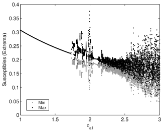
The case without cross immunity, $\epsilon=0$, reduces to a previously studied model with only ADE (LeahPRE, ; LeahJTB, ) because the cross immune and recovered compartments have the same infection rate and are treated identically. It has been shown (LeahPRE, ; LeahJTB, ) that as ADE is increased, the system undergoes a Hopf bifurcation to stable periodic oscillations and then to chaos (Fig. 2). Desynchronization between strains occurs in the regions of chaotic outbreaks, but all strains are synchronized near the Hopf bifurcation when the outbreaks are periodic. The system has been analyzed in the neighborhood of the Hopf bifurcation using a reduced model that assumes a lower dimensional, synchronized system. In the next section, we extend this analysis to the case of weak cross immunity.

Figure 2: Bifurcation diagram in ADE for the multistrain system with no cross immunity. For each ADE value, we show the local maxima (black) and local minima (gray) of the susceptibles during a 100 year time series, after removal of transients. From LeahPRE .

III Stabilizing effect of weak cross immunity

We consider first the effect of weak cross immunity, $\epsilon\ll 1$, and show that it helps stabilize the steady state. Numerical simulations indicate that when $\epsilon$ is small, the system undergoes a Hopf bifurcation as ADE is increased, as it does for the system without cross immunity, and the compartments are identical across all $n$ strains near the Hopf bifurcation. Thus the system’s dimensionality reduces. Assuming symmetry between strains, we rewrite Eqs. II as follows:

$$\frac{dy_{1}}{dt} = \mu-\beta ny_{1}y_{2}-\beta\phi n(n-1)y_{1}y_{5}$$

$$\frac{dy_{2}}{dt} = \beta y_{1}y_{2}+\beta\phi(n-1)y_{1}y_{5}-\sigma y_{2}$$

$$\frac{dy_{3}}{dt} = \sigma y_{2}-\beta(1-\epsilon)(n-1)y_{2}y_{3}$$

$$-\beta(1-\epsilon)\phi(n-1)^{2}y_{3}y_{5}-\theta y_{3}$$

$$\frac{dy_{4}}{dt} = \theta y_{3}-\beta(n-1)y_{2}y_{4}-\beta\phi(n-1)^{2}y_{4}y_{5}$$

$$\frac{dy_{5}}{dt} = \beta(1-\epsilon)y_{2}y_{3}+\beta(1-\epsilon)\phi(n-1)y_{3}y_{5}+\beta y_{2}y_{4}$$

$$+\beta\phi(n-1)y_{4}y_{5}-\sigma y_{5}$$

where $y_{1}$ represents the fraction of the population that is susceptible to the disease, $y_{2}$ the primary infectives, $y_{3}$ the cross immunes, $y_{4}$ the recovereds, and $y_{5}$ the secondary infectives. Since $\mu_{d}$ is a small parameter, for ease of analysis we set the mortality rate $\mu_{d}=0$. This approximation is equivalent to assuming that all mortality occurs in the $r_{tot}$ class, those who have recovered from infections with two serotypes. In a region where dengue is very common and dengue infections occur early compared to the human life expectancy, it may be an accurate assumption. The endemic steady state for Eqs. III is

$$y_{1} = {\frac{\sigma}{\left(1+\phi\right)\beta}}$$

$$y_{2} = {\frac{{\mu}}{\sigma\,{\it n}}}$$

$$y_{3} = \frac{\mu\,\sigma}{\beta\mu(n-1)(1-\epsilon)(1+\phi)+\theta\sigma n}$$ (3)

$$y_{4} = {\frac{{\sigma}^{2}\theta\,{\it n}}{\beta\,\left(1+\phi\right)\left[\beta\mu(1+\phi)(1-\epsilon)(n-1)^{2}+\sigma\theta n(n-1)\right]}}$$

$$y_{5} = {\frac{{\mu}}{\sigma\,{\it n}\,\left({\it n}-1\right).}}$$

Evaluating the eigenvalues of the Jacobian of Eqs. III at the steady state allows us to study its stability as a function of $\epsilon$. Since both $\mu$ and $\epsilon$ are small parameters, we expand the root of the characteristic polynomial, $P(x(\mu,\epsilon))$, of the Jacobian matrix as follows:

$$x(\mu,\epsilon)=x_{0}+x_{1}\mu+x_{2}\epsilon+x_{3}\mu^{2}+x_{4}\epsilon^{2}+x_{5}\mu\epsilon.$$ (4)

Let us also use the following transformation for the characteristic polynomial $P(x)$

$$\tilde{P}(x)=\mu P(x).$$ (5)

Substituting Eq. 4 into the characteristic polynomial and using Eq. 5, four of the five eigenvalues can be obtained:

$$\lambda_{1} \simeq -\frac{\beta}{\sigma n}(n-1)(\phi+1)^{2}\mu$$ (6)

$$\lambda_{2} \simeq -\theta$$ (7)

$$\lambda_{3/4} \simeq \pm i\sqrt{\beta}\left[1+\frac{\beta\phi(n-1)}{2n(\theta^{2}+\beta)}\epsilon\right]+$$

$$+ \frac{\beta}{2\sigma n}\left[\phi^{2}(n-1)-n(\phi+1)\right]\mu-\frac{\beta\theta\phi(n-1)}{2n(\theta^{2}+\beta)}\epsilon$$

The last eigenvalue can be obtained by performing the following substitution in the characteristic polynomial

$$P^{\prime}(x)=\mu^{5}P(x/\mu).$$ (9)

The fifth eigenvalue is then found to be

$$\lambda_{5}\simeq-\sigma.$$ (10)

The real part of the pair of complex eigenvalues $\lambda_{3/4}$ determines the stability of the system, since the other eigenvalues are clearly negative. Notice that the parameter $\epsilon$ occurs in both the real and imaginary parts of the eigenvalues. Therefore, we expect that $\epsilon$ will modify not only the stability of the endemic state but also the ensuing frequency of oscillations. To first order, the real part of $\lambda_{3/4}$ is

$$\Re[\lambda_{3/4}]=\frac{\beta}{2\sigma n}\left[\phi^{2}(n-1)-n(\phi+1)\right]\mu-\frac{\theta\beta\phi(n-1)}{2n(\theta^{2}+\beta)}\epsilon.$$ (11)

Notice that the onset of a Hopf bifurcation is clearly a function of $\mu,\epsilon$, and $\phi$. By visual inspection of Eq. 11, we see that when $\epsilon$ is increased from 0, the eigenvalue becomes more negative, so cross immunity is stabilizing in the limit of small $\epsilon$ and $\mu$.

In Figure 3, we plot the zeros of Equation 11 in $\phi$-$\epsilon$ space, showing the predicted location of the Hopf bifurcation in the presence of ADE and weak cross immunity. Below the curve, the steady state is stable. As the cross immunity is increased, a larger ADE value is needed to destabilize the steady state. Thus weak cross immunity is stabilizing. Figure 3 also shows the actual location of the Hopf bifurcation for Eqs. II. These were computed using a continuation routine (auto97, ). Note that the Hopf bifurcation in Fig. 3, where both the numerical and the analytical curves were obtained in the case of no mortality, occurs at a larger value of ADE than in the system with mortality. However, the predicted trend of stabilization due to cross immunity is observed in either case. (C.f. Figures 9-10.)

Figure 3: Predicted and actual location for Hopf bifurcation as a function of $\epsilon$ and $\phi$ for weak cross immunity in the case of no mortality ($\mu_{d}=0$). The full curve is the analytical prediction (zeros of Eq. 11), while the dashed curve is the actual location of the Hopf bifurcation, obtained numerically for the full system in the case of no mortality. The number of strains is $n=4$, and other parameters are as listed in the text.

IV Cross immunity as critical parameter

We next study numerically the effect of stronger cross immunity. We first consider the case of no ADE ($\phi=1$) and fix the number of strains to $n=4$ as for dengue. We introduce partial cross immunity by increasing the value of $\epsilon$ continuously from $\epsilon=0$ (no cross immunity) to $\epsilon=1$ (complete cross immunity). The attracting bifurcation structure is depicted in Fig. 4.

Figure 4: Bifurcation diagram for the system of ODEs (Eq. II), in absence of ADE ($\phi=1$). The cross immunity parameter $\epsilon$ is varied from $0$ to $1$. For each cross immunity value we plot the maxima (black) and the minima (gray) of the susceptibles during a 100 year time series, after removal of a transient. A transition to chaos occurs at $\epsilon\approx 0.2$.

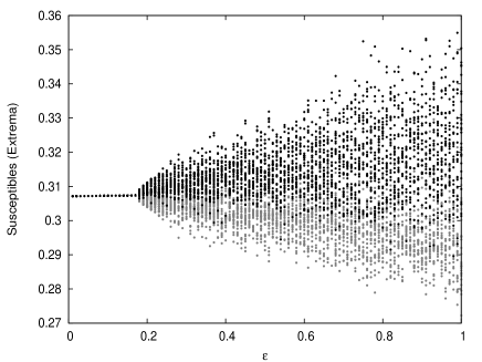
For weak cross immunity, the endemic steady state is stable. A loss of stability occurs at $\epsilon_{H}=0.165$. Numerical analysis of the eigenvalues of the Jacobian of Eqs. II at the steady state shows that a super-critical Hopf bifurcation occurs, and simulations show that the periodic orbit that appears just past the Hopf point is stable over a very small range of $\epsilon$. The strains are desynchronized on the periodic branch, so it is not possible to analyze this bifurcation using a reduced model as in Section III. Also in contrast to the Hopf bifurcation for weak cross immunity studied in the previous section, for which one complex pair of eigenvalues loses stability, at the Hopf bifurcation $\epsilon_{H}$ three identical complex pairs of eigenvalues become unstable simultaneously (GolSte85, ).

For $\epsilon_{H}<\epsilon<\epsilon_{c}$, where $\epsilon_{c}\approx 0.20$, the system displays quasiperiodicity. Figure 5 shows a Poincaré map for $\epsilon=0.179$, where the system is quasiperiodic. The map is obtained as follows: in the $n-$dimensional phase space an $n-1-$ dimensional surface is introduced by fixing the value of one of the variables, in this case the number of primary infectives currently infected with strain $1$, $x_{1}$. We then sample the other variables every time their path crosses the hyper-plane, that is, every time $x_{1}$ is identical to a fixed value. If the system is periodic, then the Poincaré map would result in a point, whereas if the system is quasiperiodic we obtain a closed curve, which is indeed what happens for the times series of Figure 5. We have observed two attracting quasiperiodic attractors with overlapping regions of stability. Sample time series for the quasiperiodic attractors are shown in Figure 6(a),(c). The four strains are desynchronized on the quasiperiodic attractors, but with different phase dynamics.

Figure 5: Poincare section showing $x_{2}(n+1)$ vs $x_{2}(n)$. $\epsilon=0.179$, $\phi=0$. See text for details.

Figure 6: Quasiperiodic attractors for $\epsilon=0.179$ (panels a,b) and $\epsilon=0.2$ (panels (c),(d)). Time series of primary infectives (log variables) are shown in (a),(c). Phase differences of primary infectives $x_{2},x_{3},x_{4}$ relative to primary infective $x_{1}$ are shown in (b),(d). The time series in (a),(c) are the beginning of those used to generate (b),(d). The reference strain $x_{1}$ is the lightest gray curve in (a),(c). Other parameters: $\phi=1$.

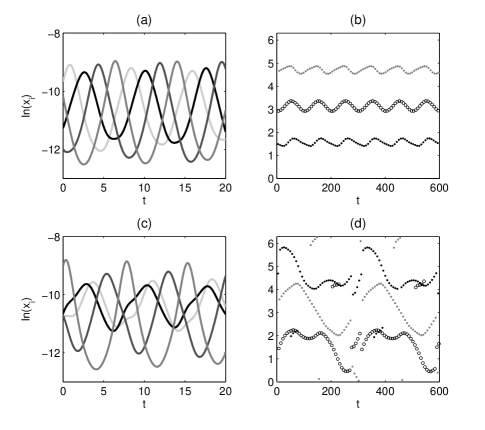
To study the strain desynchronization in more detail, we define a phase difference between compartments, as in LeahPRE . Let $Y(t)$ be the reference compartment and $Z(t)$ another compartment. Let $\{t_{k}\}$ denote the sequence of times for local maxima of $Y(t)$ and $\{\tau_{k}\}$ the sequence of times for local maxima of $Z(t)$. For $\tau_{m}\in(t_{k},t_{k+1})$, define the phase of $Z$ relative to $Y$ as $\Psi_{ZY}(\tau_{m})=2\pi\frac{\tau_{m}-t_{k}}{t_{k+1}-t_{k}}$. The phases of the other primary infective compartments relative to $x_{1}$ for the quasiperiodic attractors are shown in Figure 6(b),(d). For the attractor at weaker cross immunity, the phases of the strains relative to each other are approximately constant. This is sometimes called a splay phase state in the coupled oscillator literature. In contrast, the behavior at stronger cross immunity is more complex and qualitatively different, with the order of the strain outbreaks changing over time. Finally, since all the strains have identical parameters, we note that any permutation of strain labels gives another similar quasiperiodic state.

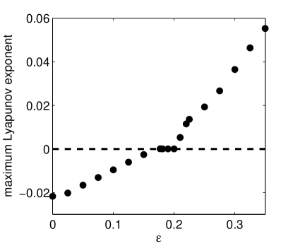
When the cross immunity is increased above $\epsilon_{c}\simeq 0.20$, the system bifurcates to chaos. The presence of chaos in SIR multistrain models with cross immunity has been already revealed by several studies in the past (KamSas02, ; GupEtAl98, ; AndLinLev97, ; EstVar03, ). We have confirmed the chaotic behavior by computing the maximum Lyapunov exponent for Eqs. II. The maximum Lyapunov exponent was obtained by integrating the linear variational equations along solutions to Eqs. II for $10^{4}$ years after removal of transients. Results are shown in Fig. 7. For $\epsilon<\epsilon_{H}$, the endemic steady state is stable and the maximum Lyapunov exponent is negative. For $\epsilon\in(\epsilon_{H},\epsilon_{c})$, the system exhibits quasiperiodic solutions and the maximum Lyapunov exponent is zero. For $\epsilon>\epsilon_{c}$, the system is chaotic and positive Lyapunov exponents are observed.

Figure 7: Maximum Lyapunov exponent of Eqs. II for $\phi=1$ as a function of cross immunity strength $\epsilon$. Equations were integrated for $10^{4}$ years after removal of transients.

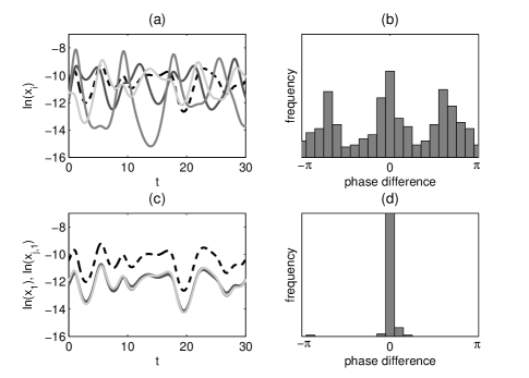
Sample time series for chaotic solutions are shown in Fig. 8(a),(c). Panel (a) shows the four primary infective compartments, which are desynchronized. We measured the phase differences of the other primary infectives relative to primary infective $x_{1}$, and they are frequently nonzero, although there appears to be some structure with certain phase differences more probable than others, as shown in Fig. 8(b). Figure  8(c) shows times series of all primary and secondary infective compartments that are currently infected with strain 1. We observe that primary and secondary infective compartments infected with the same strain (i.e., $x_{i}$ and the three $x_{j,i}$ compartments, where $j\neq i$) are usually synchronized. Figure 8(d), a histogram of phase differences of the $x_{j1}$ relative to $x_{1}$, shows the synchronization more clearly. This effect has been observed previously for the model with ADE only (LeahPRE, ) and has been explained by a collapse of the dynamics onto a lower dimensional center manifold (LeahJMB, ). The same reduction in dimension is observed in the system with cross immunity (Figure 8) as well as in the system with both ADE and cross immunity (data not shown).

Figure 8: Chaotic attractor for $\epsilon=0.35,\phi=1$. (a) Time series of all four primary infectives (log variables). Black dashed curve: $x_{1}$; darkest gray curve: $x_{2}$. (b) Histogram of phase differences of primary infective $x_{2}$ relative to primary infective $x_{1}$. (c) Time series of the first primary infective $x_{1}$ and the secondary infectives currently infected with strain 1 $x_{j,1}$ (log variables). Black dashed curve: $x_{1}$. (d) Histogram of phase differences of secondary infective $x_{2,1}$ relative to primary infective $x_{1}$. Phase difference histograms are collected for 2000 year time series.

V Interaction of strong cross immunity and ADE

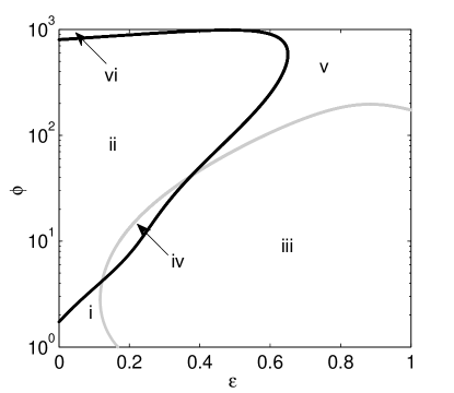
We now turn to the interaction of both ADE and cross immunity, computing bifurcation diagrams using a continuation routine (auto97, ). Figure 9 shows the full bifurcation diagram in $\phi$-$\epsilon$ space. Here, the cross immunity ranges from 0 to 1. The vertical axis is a logarithmic scale for $\phi$. The curves show the parameters of $(\epsilon,\phi)$ at which a Hopf bifurcation occurs. However, the curves denote different types of stability exchange. When crossing the black curve, only one pair of eigenvalues crosses the imaginary axis, indicating a simple bifurcation to or from periodic orbits. In contrast, when crossing the gray curve, the situation is degenerate in that 3 identical pairs of eigenvalues cross the imaginary axis. In this case, it is expected that complicated dynamics such as torus bifurcations may come into existence. For example, when traversing regions i, ii, and vi by increasing $\phi$, we go from steady state through a periodic orbit and possibly aperiodic behavior, and then through another Hopf bifurcation to return to a steady state. On the other hand, if we go from region iii to v by increasing $\phi$, we go from periodic or aperiodic behavior through a reverse degenerate Hopf bifurcation to steady state.

Notice that there are two relatively large regions of stable steady behavior: one for small $\epsilon$ and small $\phi$ in region i, and one for large $\epsilon$ and large $\phi$ in region v. (Note that the latter region of stable endemic states extends to small $\epsilon$ and large $\phi$, labelled region vi in the figure.) For large cross immunity where $\epsilon$ is between 0.65 and 1, a sufficiently large value of $\phi$ will stabilize the steady state state again. However, the value of $\phi$ is so large (the Hopf bifurcation has values of $\phi$ on the order of 100) that it is unrealistic. Therefore, to explore in more detail the bifurcations occuring at reasonable values of $\phi$, we examine the case where $\epsilon$ is small, which is shown in Fig. 10.

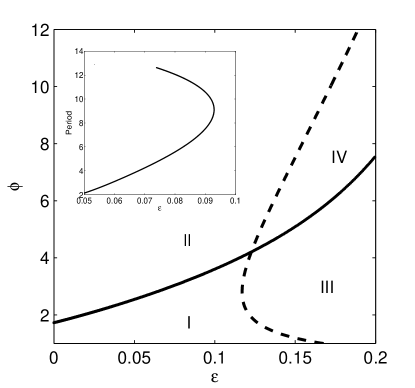
In Fig. 10, there are four distinct regions describing the stability of the steady state behavior. In region I, the endemic steady state is stable. The solid curve is a line of Hopf bifurcations where one complex pair of eigenvalues becomes unstable. The dashed curve is a line of Hopf bifurcations where three identical complex pairs of eigenvalues become unstable. Therefore, the system has zero unstable eigenvalues in region I, one unstable pair in region II, three unstable pairs in region III, and four unstable pairs in region IV. At the Hopf bifurcation between regions I and II, a stable periodic orbit emerges for which all four strains are synchronized and identical. This bifurcation was studied in Section III using a reduced model that assumed symmetry between the strains. This periodic orbit has a narrow region of stability, and then it quickly bifurcates to chaos, so the majority of region II displays chaotic dynamics. At the Hopf bifurcation between regions I and III, the region of stable periodic orbits is even smaller, and then the system goes to a quasiperiodic attractor. When $\epsilon$ becomes sufficiently large, the system bifurcates to chaos. Although quasiperiodic orbits are observed for portions of region III shown in Figure 10, the majority of region III for $\epsilon>0.2$ displays chaotic dynamics. Chaotic dynamics are also observed in most of region IV. Figure 10 (inset) also partially explores the sensitivity of the average oscillation period in region II with respect to $\epsilon$. Here $\phi\approx 3.877$, and we vary $\epsilon$ to compute a branch of periodic orbits. Plotted is the period of the branch of periodic orbits (unstable). Notice that in the linear range near the bifurcation point where $\epsilon\in(0.05,0.07)$, the slope is on the order of 100, showing a clear sensitive dependence of the oscillation period on the cross immune response. For larger values of $\epsilon$, the period exhibits a nonlinear response at the turning point, resulting in a bi-unstable branch of periodic orbits.

Figure 9: Full bifurcation diagram in cross immunity $\epsilon$ and ADE $\phi$. Curves indicate location of Hopf bifurcations. See text for details.

Figure 10: Blowup of bifurcation diagram in Fig. 9 for small cross immunity $\epsilon$ and ADE $\phi$. Curves indicate location of Hopf bifurcations. Only region I has stable steady states. The inset shows the period of a branch of unstable orbits as a function of $\epsilon$ for $\phi\approx 3.877$ in region II. See text for details.

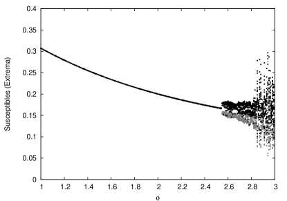
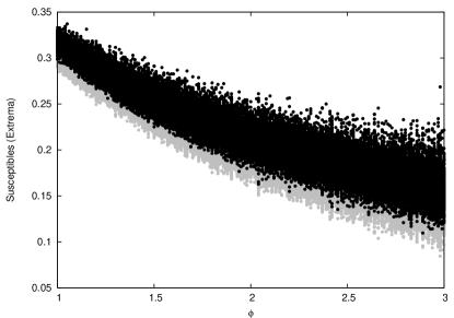
Finally, we show the interplay between ADE and cross immunity by comparing the bifurcation diagram of Figure 2, which was obtained with a model equivalent to the model of Eqs. II with no cross immunity, to the case of weak and strong cross immunity. In other words, we fixed the value of $\epsilon$ and built the bifurcation diagram using $\phi$ as critical parameter. Figure 11 shows the effect of the inclusion of weak cross immunity ($\epsilon=0.05$). By visual comparison with Figure 2, it is clear that the region of stability is increased: A value of $\phi\approx 2.5$ is needed to destabilize the system in comparison with $\phi\approx 1.7$ needed in the case of no cross immunity. Figure 11 shows the effect of strong cross immunity on the bifurcation structure ($\epsilon=0.6$). The system is observed to be chaotic for all the considered values of ADE.

Figure 11: Bifurcation diagrams in ADE for cases with nonzero cross immunity. For each ADE value, we show maxima (black) and minima (gray). 11 weak cross immunity, $\epsilon=0.05$. 11 strong cross immunity, $\epsilon=0.6$. (For comparison, Fig. 2 shows the case of no cross immunity.)

VI Conclusions and Discussion

In this work we analyzed the impact of two types of strain interactions in a multistrain model for epidemics, cross immunity and ADE. The ADE parameter measured an increase in infectiousness of secondary infectives, and the cross immunity strength determined the reduction in susceptibility to other strains during a temporary period after recovering from primary infection with one strain.

The nature of the observed dynamics depended on the strength of the cross immunity. Weak cross immunity was found to stabilize the endemic steady state. This effect was motivated analytically by studying a reduced model for weak cross immunity with symmetry between strains. Although the analysis was performed for a perturbed system without mortality, both the analytical treatment and numerical simulations of the full system were in good qualitative agreement. Since the onset of fluctuations is determined by Hopf bifurcations in models for dengue, the stabilizing effect of cross immunity shows that it is an important parameter to include when modeling disease fluctuations about equilibria. In addition, since cross immunity has a strong effect on the period of oscillation, it will play a role in determining the timing of efficient disease control strategies.

When considering strong cross immunity, most of the parameter regions predict unstable steady state behavior, as shown in Fig. 9. In fact, when the cross immunity parameter $\epsilon$ is greater than 0.65, stable endemic behavior was achieved only for unrealistically large values of ADE. As a result, strong cross immunity destabilized the system, and we observed complicated aperiodic fluctuations, such as quasiperiodic behavior and chaotic outbreaks. In contrast to the synchronized periodic behavior seen for weak cross immunity, we observed that both quasiperiodic and chaotic attractors exhibited strains that were unsynchronized. Asynchrony in chaotic outbreaks has also been observed in multistrain models with ADE and no cross immunity (LeahPRE, ).

Because time series data for dengue fever show asynchronous outbreaks for the different strains and non-periodic behavior (B:Nisalak, ), our work suggests possible refined parameter ranges for dengue in terms of ADE and cross immunity. Specifically, either the ADE or the temporary cross immunity must be strong enough to put the system in the chaotic, desynchronized region, where certain types of unstable steady states were observed. There is now a need to quantify multistrain models against existing data sets (such as B:Nisalak ) and further refine parameter estimates. It should be noted that the model presented here does not include seasonality. Because dengue is carried by mosquitoes and displays outbreaks with a seasonal component, including annual variations in the contact rate will likely be necessary for good quantitative agreement between models and data. However, other longer period components exist in the data, and are probably due to the interaction between the seasonal contact rate fluctuations and the instabilities induced by the ADE and cross imunity parameters. From the ADE model analyzed in LeahPRE ; LeahJTB , it was observed that the mean period of oscillations was very sensitive with respect to the ADE parameter. In the current work, we have also done a preliminary sensitivity analysis of the mean oscillation period on the cross immune response parameter. Here we found that small changes in $\epsilon$ may yield very large changes in the oscillation period. Therefore, in order to connect the model with measured mean periods from data, both antibody enhancement and cross immunity will play an important role in model prediction and control. In closing, there are many other modeling variations which we have omitted but will refine model fidelity in future work. These include inhomogeneity in contact rate due to spatial density variation in the mosquito populations, fluctuations in the sociological parameters such as contact, birth and death rates, as well as general stochastic fluctuations in the population itself. Such stochastic effects in finite populations, which can lead to fadeout of the disease, may also impact future disease controls.

L.B.S. and S.B. were partially supported by the Jeffress Memorial Trust. I.B.S. was supported by the Office of Naval Research and the Armed Forces Medical Intelligence Center.

References

- (1) L. J. Abu-Raddad and N. M. Ferguson. The impact of cross-immunity, mutation and stochastic extinction on pathogen diversity. Proc. R. Soc. Lond. B, 271, 2004.
- (2) B. Adams and M. Boots. Modelling the relationship between antibody-dependent enhancement and immunological distance with application to dengue. J. Theor. Biol., 242:337, 2006.
- (3) B. Adams, E. C. Holmes, C. Zhang, M. P. Mammen, S. Nimmannitya, S. Kalayanarooj, and M. Boots. Cross-protective immunity can account for the alternating epidemic pattern of dengue virus serotypes circulating in Bangkok. Proc. Natl. Acad. Sci. U.S.A., 103:14234–14239, 2006.
- (4) B. Adams and A. Sasaki. Cross-immunity, invasion and coexistence of pathogen strains in epidemiological models with one-dimensional antigenic space. Math. Biol., 210:680, 2007.
- (5) M. Aguiar and N. Stollenwerk. A new chaotic attractor in a basic multi-strain epidemiological model with temporary cross-immunity. arXiv:0704.3174, 2007.
- (6) V. Andreasen, J. Lin, and S. A. Levin. The dynamics of cocirculating influenza strains conferring partial cross-immunity. J. Math. Biol., 35:825, 1997.
- (7) L. Billings, I. B. Schwartz, L. B. Shaw, M. McCrary, D. S. Burke, and D. A. T. Cummings. Instabilities in multiserotype disease models with antibody-dependent enhancement. J. Theor. Biol., 246:18, 2007.
-
(8)
Center For Disease Control Website, 2006.
http://www.cdc.gov/ncidod/dvbid/
dengue/slideset/index.htm. - (9) D. A. T. Cummings, I. B. Schwartz, L. Billing, L. B. Shaw, and D. S. Burke. Dynamic effect of antibody-dependent enhancement on the fitness of viruses. Proc. Natl. Acad. Sci. U.S.A., 102(42):15259, 2005.
- (10) E. Doedel et al. Auto97: Continuation and bifurcation software for ordinary differential equations, 1997. Available from ftp://ftp.cs.concordia.ca/pub/doedel/auto/auto.ps.gz.
- (11) C. Esteva, L. amd Vargas. Coexistence of different serotypes of dengue virus. J. Math. Biol., 46:31, 2003.
- (12) N. Ferguson, R. Anderson, and S. Gupta. The effect of antibody-dependent enhancement on the transmission dynamics and persistence of multiple-strain pathogens. Proc. Natl. Acad. Sci. U.S.A., 96:790, 1999.
- (13) M. Golubitsky and I. Stewart. Hopf bifurcation in the presence of symmetry. Archive for Rational Mechanics and Analysis, 87:107–165, 1985.
- (14) D. J. Gubler. Epidemic dengue/dengue hemorrhagic fever as a public health, social and economic problem in the 21st century. TRENDS in Microbiology, 10:100–103, 2002.
- (15) D. J. Gubler, W. Suharyono, R. Tan, M. Abidin, and A. Sie. Viremia in patients with naturally acquired dengue infection. Bull. World Health Org., 59:623–630, 1981.
- (16) S. Gupta, N. Ferguson, and R. Anderson. Chaos, persistence, and evolution of strain structure in antigenically diverse infectious agents. Science, 280:912, 1998.
- (17) B. Guy and J. W. Almond. Towards a dengue vaccine: Progress to date and remaining challenges. Comparative Immunology Microbiology And Infectious Diseases, 31:239–252, 2008.
- (18) S. B. Halstead. Dengue. The Lancet, 370:1644, 2007.
- (19) S. B. Halstead and J. Deen. The future of dengue vaccines. The Lancet, 360:1243–1245, 2002.
- (20) S. B. Halstead and E. J. O’Rourke. Antibody-enhanced dengue virus infection in primate leukocytes. Nature, 265:739, 1977.
- (21) B. L. Innis. Dengue and Dengue Hemorragic Fever. CABI, Wallingford, Oxfordshire, U.K., 1997.
- (22) M. Kamo and A. Sasaki. The effect of cross-immunity and seasonal forcing in a multi-strain epidemic model. Phys. D, 165:228, 2002.
- (23) I. Kawaguchi, A. Sasaki, and M. Boots. Why are dengue virus serotypes so distantly related? Enhancement and limiting serotype similarity between dengue virus strains. Proc. R. Soc. London Ser. B, 270:2241, 2003.
- (24) Y. Nagao and K. Koelle. Decreases in dengue transmission may act to increase the incidence of dengue hemorrhagic fever. Proc. Natl. Acad. Sci. U.S.A., 105:2238–2243, 2008.
- (25) A. Nisalak, T. P. Endy, S. Nimmannitya, S. Kalayanarooj, U. Thisayakorn, R. M. Scott, D. S. Burke, C. H. Hoke, B. L. Innis, and D. W. Vaughn. Serotype specific virus circulation and dengue disease in Bangkok, Thailand from 1973 to 1999. Am. J. Trop. Med. Hyg., 68:191–202, 2003.
- (26) M. Nuño, Z. Feng, M. Martcheva, and C. Castillo-Chavez. Dynamics of two-strain influenza with isolation and partial cross-immunity. SIAM J. Appl. Math,, 63(3):964, 2005.
- (27) S. B. Sabin. Research on dengue during World War II. Am. J. Trop. Med. Hyg., 1:30, 1952.
- (28) I. B. Schwartz, L. B. Shaw, D. A. T. Cummings, L. Billings, M. McCrary, and D. S. Burke. Chaotic desynchronization of multistrain diseases. Phys. Rev. E, 72:066201, 2005.
- (29) L. B. Shaw, L. Billings, and I. B. Schwartz. Using dimension reduction to improve outbreak predictability of multistrain diseases. J. Math. Biol., 55:1, 2007.
- (30) H. J. Wearing and P. Rohani. Ecological and immunological determinants of dengue epidemics. Proc. Natl. Acad. Sci. U.S.A., 103(31):11802, 2006.
(31)
W. H. O. website, 2006.
http://www.who.int/mediacentre/factsheets/fs117/en/. -
(32)
http://w3.whosea.org/en/Section10/Section332/ Section520_2417.htm.