A Comparison of Six Photometric Redshift Methods Applied to 1.5 Million Luminous Red Galaxies
Abstract
We present an updated version of MegaZ-LRG (Collister et al., 2007) with photometric redshifts derived with the neural network method, ANNz as well as five other publicly available photo-z codes (HyperZ, SDSS, Le PHARE, BPZ and ZEBRA) for 1.5 million Luminous Red Galaxies (LRGs) in SDSS DR6. This allows us to identify how reliable codes are relative to each other if used as described in their public release. We compare and contrast the relative merits of each code using 13000 spectroscopic redshifts from the 2SLAQ sample. We find that the performance of each code depends on the figure of merit used to assess it. As expected, the availability of a complete training set means that the training method performs best in the intermediate redshift bins where there are plenty of training objects. Codes such as Le PHARE, which use new observed templates perform best in the lower redshift bins. All codes produce reasonable photometric redshifts, the 1- scatters ranging from 0.057 to 0.097 if averaged over the entire redshift range. We also perform tests to check whether a training set from a small region of the sky such as 2SLAQ produces biases if used to train over a larger area of the sky. We conclude that this is not likely to be a problem for future wide-field surveys. The complete photometric redshift catalogue including redshift estimates and errors on these from all six methods can be found at www.star.ucl.ac.uk/mbanerji/MegaZLRGDR6/megaz.html
keywords:
Methods: data analysis – Galaxies: distances and photometric redshifts1 Introduction
Photometric redshifts will be one of the key ingredients for us to improve our understanding of the Universe in the decade to come. Up to date, galaxy large scale structure surveys relied mainly on spectroscopic redshifts to produce high precision power spectrum measurements of the galaxy distribution (e.g. Cole et al., 2005; Percival et al., 2007). Combined with CMB experiments these surveys have provided evidence that the Universe is flat and is likely to be dominated by a dark energy component (Komatsu et al., 2008).
However having a considerable step up in the size of the spectroscopic surveys will be a hard task to achieve for technical reasons. Several Multi-fibre optical spectrographs are currently being built (FMOS) (Dalton et al., 2006) or being designed (WFMOS), but it is unlikely that they will be able to survey a considerable part of the sky. On the other hand radio interferometers may be able to perform spectroscopic surveys of the sky reasonably quickly (Blake et al., 2004; Abdalla & Rawlings, 2005) but the timescale for the technical advances to allow for this will be relatively long.
The alternative to a full spectroscopic survey is to obtain multi-colour images of the sky and perform photometric redshift estimates for the galaxies we have available (e.g. Csabai et al., 2003). In a pilot study with high redshift Luminous Red Galaxies (LRGs) it has been shown (Padmanabhan et al., 2006; Blake et al., 2007) that producing large scale measurements with photometric redshifts is possible and competitive with a smaller spectroscopic redshift survey. Using the same dataset Blake et al. (2008) have shown that photometric redshifts can also be used to study small scale halo model signatures.
On the other hand there are many caveats of photometric redshifts that have to be assessed in order for us to be completely confident that these measurements are reliable to the level of systematics that we expect in future surveys. For instance Blake et al. (2007) have performed a detailed study of whether star-galaxy separation influences the cosmological measurements given that the LRGs that have been selected are contaminated at the per cent level by M-type stars which have similar colours. They have also assessed whether there is a significant contamination from dust corrections in the galaxy, by obtaining estimates of the power spectrum in different regions of obscuration in the sky.
We extend this analysis concentrating on the level of systematic effects that is introduced by the use of different photometric redshift techniques. We have selected the same sample as was selected in the MegaZ-LRG catalogue (Collister et al., 2007) and used several different photometric redshift techniques on the same galaxies available from the literature, including artificial neural networks, template fitting techniques and Bayesian techniques. We note here that LRGs have well defined 4000 break, hence this strong feature makes photometric redshift estimation an easier task. Here all codes compared produce reasonable photometric redshifts and we are comparing more subtle differences between codes.
In Sec.2 we describe the MegaZ-LRG data used. In Sec.3 we describe all the methods we have used to estimate the photometric redshifts for the LRG sample. In Sec.4 we compare different statistics for the different photo-z results. We perform an analysis to check for gradients across the sky which could arise from training sets if they only belong to a small area of the sky in Sec.5 and we present the catalogue in Sec.6. Our conclusions are drawn in Sec.7.
2 Data
We use galaxy photometry in a DR6 equivalent to the MegaZ-LRG catalogue, a photometric-redshift catalogue of Luminous Red Galaxies based on the imaging component of the SDSS 4th Data Release. The construction of this catalogue follows the same prescription as in Collister et al. (2007). Here we only outline briefly the description of the catalogue. For details on the construction of this catalogue see Collister et al. (2007).
| Code | Authors | Method | Web link |
|---|---|---|---|
| HyperZ | Bozonella et al. | Template | http://webast.ast.obs-mip.fr/hyperz/ |
| SDSS template | SDSS pipeline | LRG Template | N/A code obtained from N. Padmanabhan |
| BPZ | Benitez | Template + Bayesian priors | http://acs.pha.jhu.edu/txitxo/bpzdoc.html |
| ANNz | Collister & Lahav | Neural Networks | http://zuserver2.star.ucl.ac.uk/lahav/annz.html |
| ZEBRA | Feldmann et al. | Template, Bayesian, Hybrid | www.exp-astro.phys.ethz.ch/ZEBRA |
| Kcorrect | Blanton | Model templates | http://cosmo.nyu.edu/blanton/kcorrect/ |
| Le PHARE | Arnouts & Ilbert | Template | www.oamp.fr/people/arnouts/LE_PHARE.html |
| EAZY | Brammer at al. | Template | www.astro.yale.edu/eazy/ |
| LRT Libraries | Assef et al. | Template | http://www.astronomy.ohio-state.edu/rjassef/lrt/ |
2.1 Selection criteria
The MegaZ-LRG catalogue is selected from the SDSS imaging database using a series of colour and magnitude cuts (Collister et al., 2007) which were designed to match the selection criteria of the 2dF-SDSS LRG and Quasar (2SLAQ) survey (Cannon et al., 2006). 2SLAQ is a spectroscopic follow-up combining the SDSS photometric survey and the spectroscopy from the Two-degree Field (2dF) instrument of the Anglo-Australian Telescope (AAT).
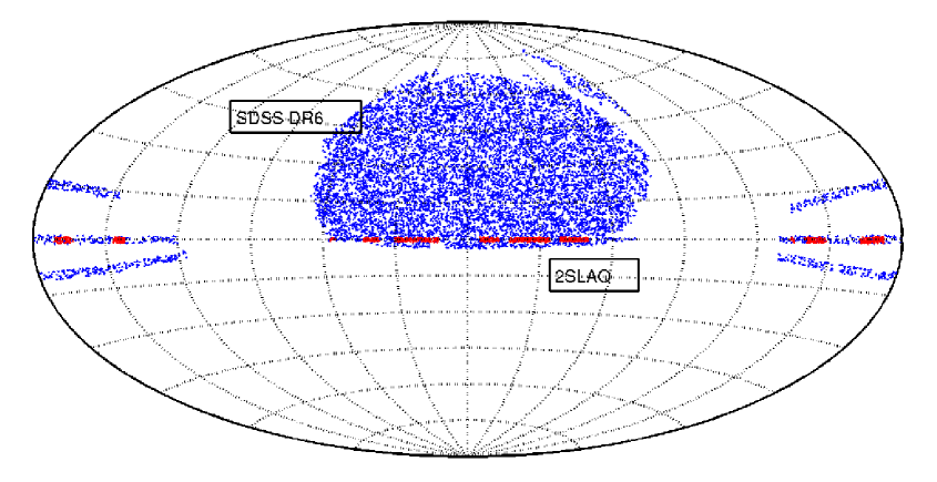
The spectroscopic redshifts available from 2SLAQ were used to train and test the photometric redshift code, which we then applied to the entire set of LRGs selected from the SDSS imaging database. Around objects in selected fields of the SDSS equatorial stripe (at declination ) were available. The 2SLAQ survey demonstrated that these selection criteria are efficient in the identification of intermediate-redshift LRGs. The most significant contaminant, accounting for virtually all of the remaining of objects, is M-type stars.
The 2SLAQ selection criteria fluctuated a little at the beginning of the survey. Specifically, the faint limit of the -band magnitude , and the minimum value of (a colour variable used to select LRGs), were varied slightly. For the majority of the 2SLAQ survey, the criteria and were used. For further details on this see (Cannon et al., 2006).
We note that our training sub-sample is extrapolated in sky position. The 2SLAQ targets lie exclusively in the equatorial stripe at declination , so may not fully trace effects such as dust extinction which depend on sky co-ordinate. One of the important aims of this study is to assess how much this sky extrapolation biases the final photo-z measurements with a training set method.
3 Photometric redshifts estimators
This section describes how we obtained the photometric redshifts for 5482 galaxies in the 2SLAQ sample. We have subdivided the galaxies from 2SLAQ into a training sample and a testing sample. The training sample was used to train the training part of the codes presented here. The rest of the sample was chosen to be 5482 so that enough galaxies were left in the training sample. These galaxies were randomly chosen. Only these galaxies were used to test the codes final accuracy, hence there being less galaxies than the 13000 galaxies available to test the codes.
We have used several different codes in the literature to provide photometric redshift estimates as well as redshift errors for a subsection of the 2SLAQ sample. The rest of the sample was used by some of the methods as a training set and therefore we do not use those galaxies in the comparison as this might introduce biases in our study.
We emphasise here that the comparison we are undertaking is a high level comparison; i.e. we are comparing end products without decomposing the problem into smaller parts in order to potentially assess where discrepancies are arising, in other words comparing codes as black boxes. Therefore the comparison is a comparison of the ensemble of codes plus galaxy libraries used with each code. We argue that this is a valid comparison as this is what a naive user of these publicly available codes would get should they choose one code rather than another. We also argue that a full analysis is needed to have the highest level of confidence in photometric redshifts and believe that this is being done by the Photometric accuracy testing program (PHAT) collaboration111http://www.astro.caltech.edu/twiki_phat/bin/view/.
3.1 Methodology: codes considered in this work
We give here a brief description of the codes we have used in this work. For a more general description of photo-z methods we refer the reader to Lahav et al. (2008) and Budavari (2008).
3.1.1 SDSS template fitting code.
The template-fitting technique in photometric redshift estimation is a fit between the data and a given set of templates for those galaxies. For the purpose of redshift estimation, the galaxy templates usually come from stellar population synthesis models (e.g. Fioc & Rocca-Volmerange, 1997; Bruzual & Charlot, 2003). A linear combination of templates is used. The coefficients of the templates are the free parameters for the minimisation. We note the set of templates observed at redshift z and the observed flux in filter with error of . The photometric redshift is found via
| (1) |
where is the flux of spectrum through filter .
The greatest disadvantage of this method (which also applies to all the other template fitting techniques presented here) is the potential mismatch between the templates used for the fitting and the properties of the sample of galaxies for which one wants to estimate the redshifts. A hybrid method can be used, in which in order to calibrate the templates to a better representation of the studied galaxy sample one would use a training set with known spectroscopic redshifts and similar properties to the galaxies whose redshifts need to be estimated. The SDSS code used here applies a hybrid method to the LRG sample using a modified elliptical galaxy template, adjusted to represent an LRG spectrum after three iterations of correction. Given that early type galaxies evolve passively, only one template is used in the code.
3.1.2 HyperZ
HyperZ (Bolzonella et al., 2000) was the first publicly available photo-z code and has consequently been widely used in the literature for photometric redshift estimation. It is a simple template fitting code that can be used in conjunction with two sets of basis SEDs, namely the observed Coleman et al. (1980) templates (CWW hereafter) or the synthetically generated Bruzual & Charlot (2003) templates (BC hereafter). HyperZ takes as its inputs the photometric catalogue of galaxies with magnitudes and errors on magnitudes through the different filters specified in the filter set, as well as a list of spectral templates to be used in the minimisation. Various different reddening laws can also be implemented in order to account for the effect of interstellar dust on the shape of the SED. The damping of the Ly forest increasing with redshift is modelled according to Madau (1995). We have experimented with a variety of different basis template sets including the four CWW templates and interpolations between them as well as the 8 synthetic BC templates. We find the BC templates to produce considerably better photo-z’s than the CWW and interpolated CWW template sets. In order to demonstrate the effects of using two different template sets to calculate photometric redshifts with the same code, we present results obtained using both the four CWW templates roughly corresponding to types E,Sbc,Scd and Im and the eight BC templates roughly corresponding to types Single Burst, E, S0, Sa, Sb, Sc, Sd and Im.
We have also considered the photo-z outputs with no correction for galactic reddening and with a Calzetti reddening law (Calzetti et al., 1994) applied to the templates for all the template sets considered. In all cases we find that including an extinction correction slightly worsens the photometric redshift estimate. Our final HyperZ outputs therefore make no correction for the galactic extinction.
We used magnitudes in all five SDSS optical bands even though the photometric uncertainties in the -band are large and therefore would contribute to a larger scatter in the photo-z estimate. We have checked that removing the -band data does in fact worsen the photo-z estimate.
We note here that other template-based methods are also available for photo-z estimation such as ImpZ (private communication: M. Rowan-Robinson), k-correct (Blanton & Roweis, 2007), EAZY (Brammer et al., 2008) and the LRT Libraries (Assef et al., 2008). These have not been presented in this comparison.
3.1.3 ANNz
When a representative training set is available training methods become a viable option to use instead of template-fitting methods. The basic principle of training methods is the derivation of a parameterisation of redshift through the magnitudes of the galaxies in a training set. This parameterisation is then applied to galaxies for which no spectroscopy is available, yielding an estimate of the photometric redshift. One of the training methods used here is Artificial Neural Networks (Collister & Lahav, 2004). Neural networks have been used for estimation of photo-z in data (Collister et al., 2007) as well as forecasts of photometric redshifts for future data (Banerji et al., 2008; Abdalla et al., 2008). An artificial neural network is made up of several layers, each consisting of a number of nodes. The first layer receives the galaxy magnitudes as inputs, while the last layer outputs the estimated photometric redshift. The layers in between could consist of any number of nodes each. The nodes are interconnected so that a node in a given layer is connected to all nodes in the adjacent layers, every connection carrying a weight , where i and j describe the two nodes. Each node i is assigned a value and an activation function
| (2) |
is evaluated.
The value of a subsequent node j is then calculated as the summation of the weighted values of the activation functions of all nodes i pointing to it:
| (3) |
When a network is trained the weights of all node connections are determined by minimising a cost function E evaluated on the training set of galaxies where
| (4) |
and photometric input of for galaxy k from the training set is , and the spectroscopic redshift of the galaxy is .
To avoid an over-fitting, every network is tested on a validation set of galaxies, whose spectroscopic redshifts are also known. The network with lowest value of E as calculated on the validation set is selected and the photometric sample is run through it for redshift estimation (Collister & Lahav, 2004).
The artificial neural networks used in ANNz can be described as follows: , where and are respectively the number of input and output parameters, while is the number of nodes in the intermediate layer. In the case of photometric redshift estimation using MegaZ-LRG, a network of the form 5:10:10:1 was used, this was found empirically to be optimal (Firth et al., 2003; Collister et al., 2007).
|
|
|
 |
3.1.4 BPZ
An extension of the above HyperZ likelihood () approach is to incorporate priors, with the Bayesian framework. Benítez (2000) formulated the problem as follows. The probability of a galaxy with colour and magnitude having a redshift is
| (5) |
where the term is the conventional redshift likelihood employed e.g. by Hyper-z, and is just a normalisation. The new important ingredient is , which brings in the prior knowledge of the magnitude redshift distribution. With the aid of the extra information (prior), this approach is effective in avoiding catastrophic errors of placing a galaxy at an unrealistic redshift.
BPZ can function in a Bayesian and Maximum Likelihood (ML hereafter) module and therefore produces two outputs for the photometric redshift. The ML method simply picks the highest maximum over all the likelihoods as its redshift estimate whereas the Bayesian method averages over all the likelihoods after weighting them by their prior probabilities.
BPZ also takes as its input a photometric catalogue with magnitudes in different filters and their corresponding errors. The BPZ templates include the four CWW templates as well as the spectra of two star-bursting galaxies from Kinney et al. (1996). In this study we added nine interpolations between each of the four CWW templates to the BPZ template list to produce a more complete list of basis SEDs. This gives us a set of 38 basis templates for BPZ to use. We find that 17 of these templates concentrated towards the early types are sufficient to produce the best photometric redshift estimate. Adding more templates does not improve the photo-z scatter. We also used two further points of interpolation between each of the templates in colour space as specified by the INTERP parameter in BPZ. A flat prior was used throughout the calculation resulting in very similar results from the Bayesian and ML runs.
The BPZ output includes two photo-z estimates from the Bayesian and ML runs as well as a quantity called that is the amount of probability contained between and around the Bayesian photo-z estimate. In order to select galaxies which only have a single compact peak in their probability distribution, we need to consider those galaxies with at the very least and for a robust estimate (private communication: N.Benitez). In the first case, we select out 4811 of the 5482 galaxies and in the second case we are left with 3689 of the 5482 galaxies. The Bayesian output from BPZ with galaxies with selected, gives us the best photo-z estimate and it is this result that we use as the BPZ output in the plots.
3.1.5 Le PHARE - PHotometric Analysis for Redshift Estimations
Le PHARE is very similar to HyperZ in that a set of template SEDs together with a filter set are used to determine a set of model magnitudes used in the photometric redshift calculation. These are then compared to the observed magnitudes using a minimisation in order to compute the redshift of an object. The Le PHARE package includes various template sets used to construct the library of model magnitudes. These include the Coleman, Wu and Weedman and Kinney star-burst templates, an extended CWW template set with 72 interpolations between the standard CWW templates, 42 synthetic GISSEL templates as well as the observed templates of Poggianti. We have experimented with using these various template sets for photo-z estimation on our sample of 5482 2SLAQ objects and find the best photometric redshifts to be obtained with the 8 Poggianti templates corresponding to galaxy types Ell, S0, Sa, Sb, Sc, Sd, SB2 and SB1. The 42 GISSEL templates give slightly worse photo-z’s than the Poggianti templates but the scatter on the photometric redshift when using the extended sample of 72 interpolated CWW templates is 30% worse than that obtained using the 8 Poggianti templates. Therefore we can see that in a template-based method, we do not necessarily gain in redshift accuracy by adding more model SEDs to our library.
Le PHARE also includes various prescriptions to correct for galactic extinction. We have tried running Le PHARE with different extinction laws assuming E(B-V)=0.034 and find that in all cases, the photo-z estimate is worse when we include the effects of galactic extinction. Our final Le PHARE output is therefore obtained using the 8 Poggianti templates and neglecting the effects of galactic extinction. We use 5-band photometry in the SDSS filters as this gives significantly more accurate photometric redshifts compared to if we remove the -band photometry with the largest photometric errors.
3.1.6 ZEBRA - Zurich Extragalactic Bayesian Redshift Analyzer
The Zurich Extragalactic Bayesian Redshift Analyzer (Feldmann et al., 2006) is a more sophisticated Bayesian template-fitting photometric redshift code compared to its predecessor, BPZ. The basic principles of estimating redshifts using templates and Bayesian priors remains as described in §3.1.4 but among the novel techniques employed within the ZEBRA package are the photometry check mode that checks and corrects the photometry in certain filters, a template optimisation mode to improve the standard set of templates in specified redshift bins using a training set of galaxies with spectroscopic redshifts and the ability to calculate a prior self-consistently from the photometric catalogue when ZEBRA is run in its Bayesian mode.
We choose not to employ the photometry check mode within ZEBRA as we are fairly confident that we have reliable photometry for our objects and have checked that applying a catalogue correction does not improve the photometric redshifts.
ZEBRA’s template set consists of the standard E, Sbc, Scd and Im galaxies as well as the SEDs of the two star-bursting galaxies SB2 and SB3. These are further interpolated in logarithmic space by ZEBRA during the photo-z estimation. We find that including the E, Sbc and Scd templates produces better results than including all six templates. Furthermore, we use ZEBRA’s template optimization mode to construct improved templates from these three basis templates in two redshift bins - and . We use a regularisation parameter of and a pliantness parameter of . Feldmann et al. (2006) gives details of these parameters and how to optimise them so as to produce the most realistic templates. We do not include IGM absorption in our templates as we find that this produces better photometric redshifts. The optimisation procedure produces 39 basis templates and we use these along with our original templates in the photometric redshift calculation.
We find the Bayesian mode of ZEBRA to produce considerably better photometric redshifts than the Maximum Likelihood mode and we therefore consider only outputs from the Bayesian mode when calculating figures of merit. The Bayesian mode is run using four iterations to calculate the prior self-consistently from the photometric catalogue. Further iterations slightly worsen the photo-z estimate. We use a smoothing kernel to smooth the prior after every iteration.
4 Results
Here we summarise the results obtained when running our different public photo-z codes on the 2SLAQ sample of 5482 LRGs. Note that each of the photo-z codes detailed in 3.1 have been run several times using different parameters in order to optimise them to produce the best photo-z estimate. The final output files from each code used in this analysis are ones that gave the best photo-z estimate, hence this is not only a code comparison it is a code plus library comparison which is the final publicly available product to the non-expert on-line. We note here that this is not a comparison which is meant to contrast equal values. For instance it is already well accepted that training codes work much better within the redshift and spectral energy distribution range present in the training set but template methods are superior if there are objects in the survey outside this range. Also, codes such as BPZ provide an automatic selection of the objects with the best photo-z’s via for example the odds parameter. The purpose here is to compare the full packages, including SEDs and features available from different codes. Furthermore, the chosen sample of Luminous Red Galaxies has a very narrow range of SEDs and this comparison therefore does not highlight the strength of photometric redshift codes with a broad range of library templates that would be more suitable for other samples.
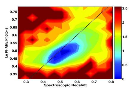
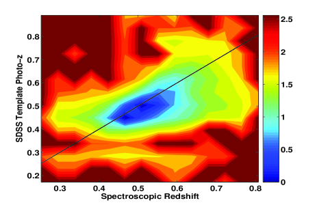
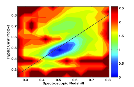
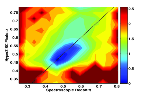
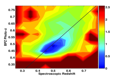
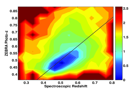
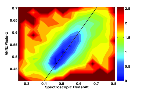
In Figure 2 we plot density plots of the spectroscopic redshift versus photometric redshift for each of these different codes. We use a redshift resolution for all codes which ensures that the main uncertainty is related to the photo-z uncertainty and not to numerical effects.
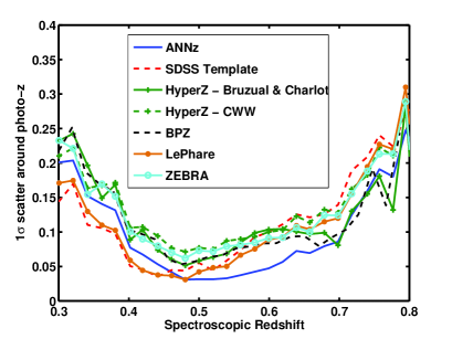
In order to evaluate the precision with which each of these different codes calculates the photometric redshift, we can look at the scatter between the true (spectroscopic) redshift and the photometric redshift. This is defined as follows:
| (6) |
This quantity is plotted in the left-hand panel of Figure 3. As expected, the empirical photo-z estimator, ANNz seems to work best at intermediate redshifts where there are a large number of representative training set galaxies. At high redshifts, HyperZ BC provides us with the best estimates of the photometric redshift. At low redshifts, the SDSS code and Le PHARE template fitting codes perform the best. We note that none of these runs used the more standard CWW templates suggesting that these templates are not a good match to the LRGs that are being analysed in this study.
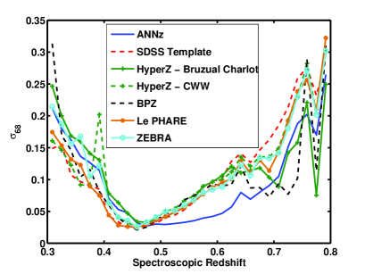
As can be seen in Figure 2 however, there are many outliers present in our sample. Another useful quantity to consider is therefore which is the interval in which 68% of the galaxies have the smallest difference between their spectroscopic and photometric redshifts. This will give us some indication of the scatter in the photometric redshift estimate once the outliers have been removed and is plotted in the right-hand panel of Figure 3.
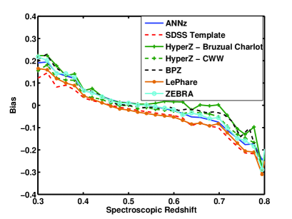
Another important quantity used to quantify how good a photo-z estimate is, is the bias defined as:
| (7) |
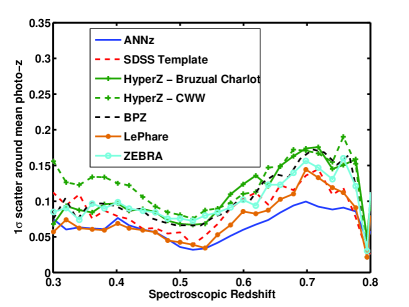
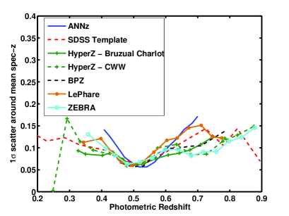
This quantity is plotted for each of the different codes, in the right-hand panel of Figure 4. Padmanabhan et al. (2005) show that galaxies with a given photometric redshift often have a systematic bias on them and this bias can therefore be added to those photo-z galaxies in order to correct for it. In order to get a feel for the error on the photometric redshift once this bias has been corrected for, we plot in the left-hand panel of Figure 4, the scatter around the mean photometric redshift estimate in each bin, defined as follows:
| (8) |
As can be seen, the scatter is now reduced for most of the codes as we are not accounting for any systematic shift that can be corrected for. The bias is largest at high redshifts for the SDSS and Le PHARE template fitting codes and these codes have the biggest improvement in the scatter at high redshifts when we take the moment around the mean rather than the true redshift.
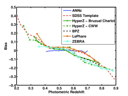
A more useful quantity in terms of future surveys is to plot the bias and scatter as a function of the photometric redshift as in Figure 5. The scatter around the mean spectroscopic redshift estimate in each photo-z bin is defined as follows:
| (9) |
We can also compare the right-hand panels of Figure 4 and Figure 5 to each other. We can see that the bias follows the same trend as a function of spectroscopic redshift for all the different photo-z codes and is fairly similar for all these codes. However, the bias as a function of the photometric redshift is very different for the different photo-z codes and more indicative of how much the photo-z estimate has to be corrected for systematic errors. This bias is almost flat for the training method which has enough training set galaxies to effectively minimise the bias through the training process. The integral under the curve is also small for ZEBRA as shown in Table 3 as the template optimisation technique here was able to remove the average bias for the entire redshift range. However, a remaining bias was found at high and low redshifts with the values of the ZEBRA configuration parameters used in this analysis222It is possible that a better choice of template optimisation parameters could be found resulting in a removal of the bias at low and high redshifts. However, as the philosophy of this paper is to perform a code comparison from the point of view of the photo-z user rather than the photo-z developer, and it is not obvious what this better choice of parameters would be, we choose to leave our results as they are..
As an alternative statistic, we present in Table.2 the fraction statistics for the methods presented in this section. The fractions are defined as the fraction of galaxies in certain regions of the photo-z/spec-z plane. If we divide this plane in rectangular regions, the fraction f0 is the fraction of galaxies which is on the diagonal of this matrix. We could have subdivided the areas along the diagonals, this would have been a suitable statistic as well. However there are reasons for which the statistic we quote is interesting. For instance if one is interested in cosmological probes where the galaxies are separated in photo-z bins then a subdivision along the photo-z axis is more natural. Given that these galaxies are relatively red with good photometric redshifts, we can see that the fraction of outliers is small for all estimators. however there is still a difference between different implementations of publicly available codes.
We also present in Table.3 the integrated bias and scatter for all the codes and libraries we have used. We can see that the training code performs best which is to be expected with a complete training set and that the bias here is very small. However this statistic does not show the redshift dependence of the scatter or bias which may be of interest depending on the application.
5 Systematic checks on the photometric catalogues
The clustering of the SDSS LRG photometric sample has been analysed using the SDSS code for photometric redshifts described in Sec.3.1.1 by Padmanabhan et al. (2006) and by ANNz described in Sec.3.1.3 Blake et al. (2007). For the rest of this section we choose to look more in detail at the effects that these two codes have on the end products of the analysis. We check for gradients in the photo-z distribution across the sky. These gradients should be present if the training set for the neural networks is biased as a function of position in the sky.
| 37% | 28% | 31% | 4% | 0.02% | |
| 27% | 31% | 37% | 4.5% | 0.8% | |
| 24% | 32% | 35% | 7% | 1.5% | |
| 26% | 32% | 32% | 7% | 1.5% | |
| 26% | 34% | 34% | 4% | 0.5% | |
| 26% | 34% | 34% | 5% | 0.8% | |
| 24% | 32% | 36% | 6% | 1% |
| 0.0575 | 0.0014 | |
| 0.0808 | -0.0264 | |
| 0.0973 | -0.0076 | |
| 0.0862 | 0.0160 | |
| 0.0718 | -0.0302 | |
| 0.0898 | 0.0013 | |
| 0.0933 | 0.0112 |
5.1 Checking for Gradients in Redshift Difference across the Sky
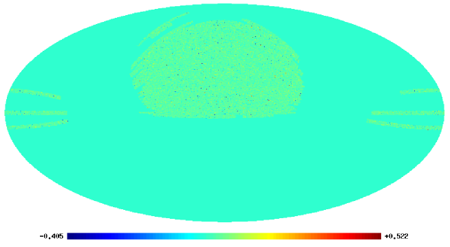
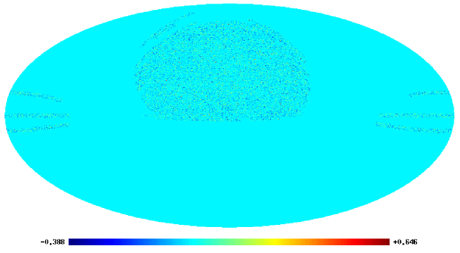
It is difficult to trust two very different techniques such as template fitting methods and training methods to produce consistent results without making a comprehensive comparison of both methods on the same set of galaxies. Given that the training set from the training method is drawn from a small region of the sky with limited range of galactic extinction one could assume a priori that this extra calibration which is necessary might introduce biases as a function of sky position in applications of empirical methods. This would be dramatic in the case of, for instance cosmological studies where we are attempting to calculate variations across the sky to infer cosmological parameters.
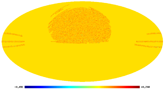
We have looked for gradients in the difference in three redshift shells, 0.4 0.5, 0.5 0.6 and 0.6 0.7. We have separated galaxies in each redshift bin according to the ANNz photometric redshift. If the separation were done with the SDSS photometric redshifts instead the result would not change a lot. The values of were taken as an average value in pixels produced with HEALPIX, hence are smoothed to produce the maps in Fig.7. No apparent gradients can be identified, in any of the redshift shells, which is an indicator for the consistency across the plane of the sky.
| objID | SDSS objID |
| ra | J2000 right ascension |
| dec | J2000 declination |
| dered_u | |
| dered_g | |
| dered_r | Dereddened model magnitudes |
| dered_i | |
| dered_z | |
| err_u | |
| err_g | |
| err_r | Magnitude errors |
| err_i | |
| err_z | |
| deVMag_i | Dereddened de Vaucouleurs magnitude |
| z_annz | ANNz photometric redshift |
| z_annz_err | ANNz photometric redshift error |
| delta_sg | ANNz galaxy probability |
| delta_err_sg | ANNz galaxy probability error |
| z_sdss | SDSS photometric redshift |
| z_hzcww | Hyper-z CWW photometric redshift |
| z_hzcww_chi | Hyper-z CWW chi squared |
| z_hzcww_errl | Hyper-z CWW photometric redshift 68% lower confidence limit |
| z_hzcww_errh | Hyper-z CWW photometric redshift 68% higher confidence limit |
| z_hzbc | Hyper-z BC photometric redshift |
| z_hzbc_chi | Hyper-z BC chi squared |
| z_hzbc_errl | Hyper-z BC photometric redshift 68% lower confidence limit |
| z_hzbc_errh | Hyper-z BC photometric redshift 68% higher confidence limit |
| z_bpz_bayes | BPz bayesian photometric redshift |
| z_bpz_errl | BPz photometric redshift 90% lower confidence limit |
| z_bpz_errh | BPz photometric redshift 90% higher confidence limit |
| z_bpz_odds | BPz bayesian odds parameter |
| z_bpz_ml | BPz maximum likelihood photometric redshift |
| z_bpz_chi | BPz chi squared |
| z_zebra | ZEBRA photometric redshift |
| z_zebra_errl | ZEBRA photometric redshift 68% lower confidence limit |
| z_zebra_errh | ZEBRA photometric redshift 68% higher confidence limit |
| z_lp | Le PHARE photometric redshift |
| z_lp_prob | Le PHARE percentage PDF between |
The different colour coding in each of the redshift shells in Fig.7 are indicative of the bias between the two methods which is of course still present, however taking that bias aside, there seems to be no correlation between the usual regions of high extinction in the SDSS regions and the scatter of biases as a function of sky position produced here. Given that the template set does not know about the training set which belongs to a selective region of the sky our conclusion is that the fact that the training set is restricted to a small region of the sky does not include significant biases as a function of sky position and therefore is not an extra source of systematic biases. This could be taken further, for instance by calculating spherical harmonics of the map above and comparing with theoretical predictions in order to estimate the actual lower bound of a potential systematic effect for a given probe but since this would involve a more specific cosmological approach we argue that this is beyond the photometric redshift comparison which is the aim of this paper.
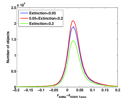
The main reason why there should be a systematic bias as a function of sky position is extinction. We have computed the difference between the two photo-z estimates for different regions of galactic extinction and plotted histograms for these quantities in Fig.6. Apart from the normalisation which encoded the fact that there are a different number of galaxies in these bins the curves are virtually identical with same bias and scatter, this also shows that there is no evidence of significant differences. This can only get better with future Planck data. So we are confident that this is not a systematic effect that will hinder future or current photometric redshift analysis.
5.2 A Photo-z comparison of the codes
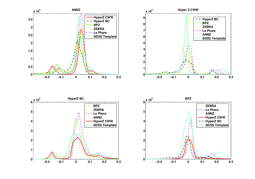
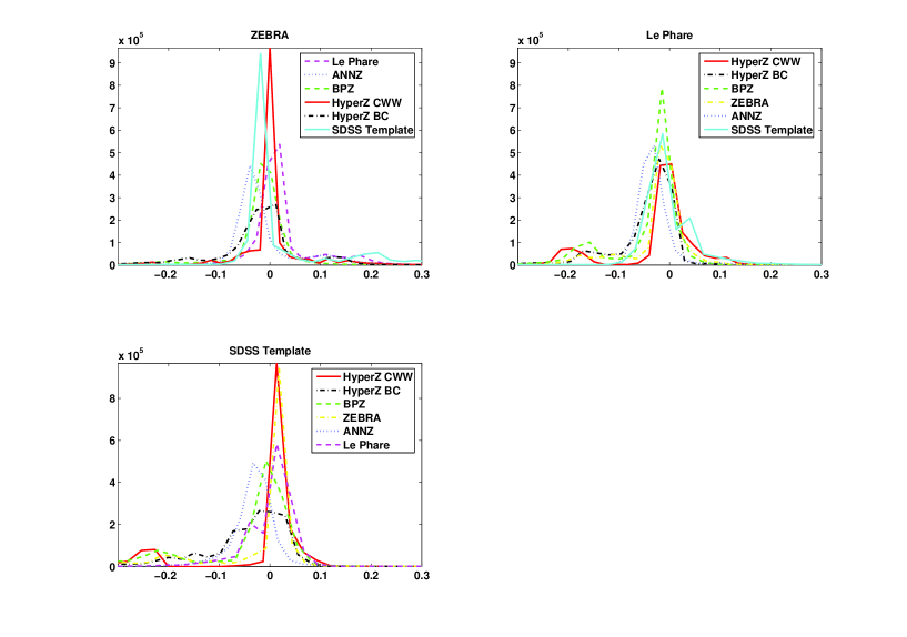
We also present here a comparison of how the photometric redshifts of each code compare to each other. We present in Fig.8 histograms of the difference between photo-z for each pair of codes that we have used in the analysis of our updated MegaZ-LRG catalogue. We can see the differences between codes is apparent in some plots.
For instance comparing ANNz to other codes there seem to be some outliers at a redshift difference of 0.1 compared to Hyperz CWW, BPZ and Hyperz BC. Similarly other pairs of codes produce outliers which indicates that this is not only a difference between template codes and training codes. We also note that for instance comparing ZEBRA with codes such as HyperZ CWW or SDSS code there is a good agreement on the scatter but there is a small bias between the codes which may suggest that the templates used might not have been optimal in some codes. The ImpZ code (private communication:M. Rowan-Robinson) was also tested on the sample of 5482 2SLAQ LRGs and produced consistent results with other template-based methods. However, as the code in its current form is not yet publicly available, we do not present these results here or extend the analysis to the MegaZ-LRG DR6 catalogue described in the next section.
We emphasise here that there are many differences even though all the photo-z estimates are of relatively good quality. There is therefore a need to deconstruct the effects of the algorithm and the template libraries in order for us to understand these differences and have even more reliable photo-z’s in the future.
6 An extension to MegaZ-LRG: catalogues with different photo-z estimators for SDSS DR-6
We have extended the photometric sample from SDSS DR4 to SDSS DR6 imaging catalogue using the same criteria devised for the 2SLAQ LRG catalogue. This extended MegaZ-LRG catalogue contains 1543596 objects over more than 8000 square degrees of the sky. As in previous studies LRGs are expected to be about 95% of the sample and M type stars are expected to be 5% of the sample. We have produced photometric redshift results for 7 different photometric redshift estimators and provided the error estimators associated with each method. We also provide trained empirical values to perform star/galaxy separation based on a set of 15 photometric parameters as in (Collister et al., 2007). All the parameters included in the revised catalogue are described in Table.4. The data can be found in the following website333www.star.ucl.ac.uk/mbanerji/MegaZLRGDR6/megaz.html.
7 Conclusions
We have presented an updated version of the MegaZ-LRG catalogue. This catalogue contains about 1.5 million objects with accurate photometric redshifts which can be used for a range of science applications. The catalogue is available on-line and contains SDSS ID information so all SDSS data can be retrieved for each object as well as the photometric redshifts from each of the six public codes.
We have run several comparisons of code and template libraries on the 2SLAQ LRG sample. We conclude that there are differences in the codes and stress that a more thorough comparison is needed where the effects of the codes and template libraries are disentangled. This will allow us to pinpoint where the discrepancies are arising. An approach based on first principles such as that presented in Budavari (2008) is also timely. We have used several figures of merit to assess which code + template library performed best for this set of galaxies. We conclude that different codes perform with different strengths depending on the figure of merit used. We outline more specifically the findings below:
-
•
As expected, the availability of a complete training set means the training method, ANNz performs best in the intermediate redshift bins where there are plenty of spectroscopic redshifts.
-
•
Le PHARE performs very well particularly in the lower redshift bins suggesting the Poggianti templates may be a better fit to LRGs at those redshifts compared to other templates used in this comparison.
-
•
HyperZ run with Bruzual & Charlot templates gives better results than using the same with CWW templates once again highlighting the importance of template choice.
-
•
The SDSS template code gives very good results compared to other codes at the highest photo-z bins despite having only one evolving template for the LRGs. Given the narrow range in SEDs of our sample of Luminous Red Galaxies, the strengths of template-based codes with extensive template libraries are not adequately highlighted by this comparison.
-
•
ZEBRA shows a small average bias indicating the importance of the template optimisation technique in removing biases.
As expected the training code performs best where the training set is large and complete and the template sets overtake the training code if the training set starts to become sparse. The importance of template choice is highlighted by the fact that most figures of merit show codes used in conjunction with the CWW templates to perform worse than those using other training or synthetic templates. This suggests that the CWW templates are not a very good match to the SEDs of these LRGs.
There is a discrepancy between the scatters found for these codes ranging from 0.057 to 0.097. Both values are considered good results for photo-z estimates as one would expect from LRGs but there is a clear difference between the different code and template combinations that are run. Given that these differences will also depend on galaxy type and training set size, it is imperative that we carry out a more thorough comparison where the effects of codes and templates are deconstructed, in order to understand what factors affect the photo-z accuracy. We caution the reader that the results presented here are specific to a sub-sample of galaxies, namely LRGs, which have a narrow range in SEDs and a complete and representative spectroscopic training set available. The conclusions presented here could and probably would change if the comparison were made with different galaxies or a different training set size.
We have also produced a set of tests to assess whether the fact that the training sets are from a restricted area in the sky affects the photometric redshifts significantly. We conclude that there is little or no difference between the results from template methods and training set methods across the sky and that the difference found is not likely to be a source of the training set being restricted in area. This is promising for future wide-field photometric redshift surveys such as the Dark Energy Survey, PanStarrs, Euclid and JDEM.
Acknowledgments
We acknowledge Stephane Arnouts, Tom Babbedge, Narciso Benitez, Micol Bolzonella, Marcella Carollo, Nikhil Padmanabhan and Michael Rowan-Robinson for useful comments regarding the publicly available codes and also for checking that our usage of the codes was acceptable. FBA acknowledges the support of a Leverhulme Early Careers Fellowship. MB is supported by an STFC studentship. OL would like to acknowledge the Royal Society Wolfson Research Merit Award.
References
- Abdalla et al. (2008) Abdalla F. B., Amara A., Capak P., Cypriano E. S., Lahav O., Rhodes J., 2008, MNRAS, 387, 969
- Abdalla & Rawlings (2005) Abdalla F. B., Rawlings S., 2005, MNRAS, 360, 27
- Assef et al. (2008) Assef R. J., Kochanek C. S., Brodwin M., Brown M. J. I., Caldwell N., Cool R. J., Eisenhardt P., Eisenstein D., Gonzalez A. H., Jannuzi B. T., Jones C., McKenzie E., Murray S. S., Stern D., 2008, ApJ, 676, 286
- Banerji et al. (2008) Banerji M., Abdalla F. B., Lahav O., Lin H., 2008, MNRAS, 386, 1219
- Benítez (2000) Benítez N., 2000, ApJ, 536, 571
- Blake et al. (2007) Blake C., Collister A., Bridle S., Lahav O., 2007, MNRAS, 374, 1527
- Blake et al. (2008) Blake C., Collister A., Lahav O., 2008, MNRAS, 385, 1257
- Blake et al. (2004) Blake C. A., Abdalla F. B., Bridle S. L., Rawlings S., 2004, New Astronomy Review, 48, 1063
- Blanton & Roweis (2007) Blanton M. R., Roweis S., 2007, AJ, 133, 734
- Bolzonella et al. (2000) Bolzonella M., Miralles J.-M., Pelló R., 2000, 363, 476
- Brammer et al. (2008) Brammer G. B., van Dokkum P. G., Coppi P., 2008, ApJ, 686, 1503
- Bruzual & Charlot (2003) Bruzual G., Charlot S., 2003, MNRAS, 344, 1000
- Budavari (2008) Budavari T., 2008, ArXiv e-prints
- Calzetti et al. (1994) Calzetti D., Kinney A. L., Storchi-Bergmann T., 1994, ApJ, 429, 582
- Cannon et al. (2006) Cannon et al. 2006, MNRAS, 372, 425
- Cole et al. (2005) Cole et al. 2005, MNRAS, 362, 505
- Coleman et al. (1980) Coleman G. D., Wu C.-C., Weedman D. W., 1980, ApJS, 43, 393
- Collister & Lahav (2004) Collister A. A., Lahav O., 2004, PASP, 116, 345
- Collister et al. (2007) Collister et al. 2007, MNRAS, 375, 68
- Csabai et al. (2003) Csabai et al. 2003, AJ, 125, 580
- Dalton et al. (2006) Dalton et al. 2006, in Ground-based and Airborne Instrumentation for Astronomy. Edited by McLean, Ian S.; Iye, Masanori. Proceedings of the SPIE, Volume 6269, pp. 62694A (2006). Vol. 6269 of Presented at the Society of Photo-Optical Instrumentation Engineers (SPIE) Conference, The UK FMOS spectrograph
- Feldmann et al. (2006) Feldmann et al. 2006, MNRAS, 372, 565
- Fioc & Rocca-Volmerange (1997) Fioc M., Rocca-Volmerange B., 1997, 326, 950
- Firth et al. (2003) Firth A. E., Lahav O., Somerville R. S., 2003, MNRAS, 339, 1195
- Kinney et al. (1996) Kinney A. L., Calzetti D., Bohlin R. C., McQuade K., Storchi-Bergmann T., Schmitt H. R., 1996, ApJ, 467, 38
- Komatsu et al. (2008) Komatsu E., Dunkley J., Nolta M. R., Bennett C. L., Gold B., Hinshaw G., Jarosik N., Larson D., Limon M., Page L., Spergel D. N., Halpern M., Hill R. S., Kogut A., Meyer S. S., Tucker G. S., Weiland J. L., Wollack E., Wright E. L., 2008, ArXiv e-prints
- Lahav et al. (2008) Lahav O., Abdalla F. B., Banerji M., 2008, Photometric Redshift Estimation: Methods and Applications. to appear in ‘Bayesian Methods in Cosmology’ ed. A. Liddle 2008.
- Madau (1995) Madau P., 1995, ApJ, 441, 18
- Padmanabhan et al. (2005) Padmanabhan et al. 2005, MNRAS, 359, 237
- Padmanabhan et al. (2006) Padmanabhan et al. 2006, astro-ph/0605302
- Percival et al. (2007) Percival et al. 2007, ApJ, 657, 645