The solar wind charge-transfer X-ray emission in the $1\over 4$ keV energy range: inferences on Local Bubble hot gas at low Z

Abstract

We present calculations of the heliospheric solar wind charge exchange (SWCX) emission spectra and the resulting contributions of this diffuse background in the ROSAT $1\over 4$ keV bands. We compare our results with the soft X-ray diffuse background (SXRB) emission detected in front of 378 identified shadowing regions during the ROSAT All-Sky Survey (Snowden et al., 2000). This foreground component is principally attributed to the hot gas of the so-called Local Bubble (LB), an irregularly shaped cavity of $\sim$ 50-150 pc around the Sun, which is supposed to contain $\sim$10⁶ K plasma. Our results suggest that the SWCX emission from the heliosphere is bright enough to account for most of the foreground emission towards the majority of low galactic latitude directions, where the LB is the least extended. On the other hand, in a large part of directions with galactic latitude above 30 degrees the heliospheric SWCX intensity is significantly smaller than the measured one. However, the SWCX R2/R1 band ratio differs slightly from the data in the galactic center direction, and more significantly in the galactic anti-centre direction where the observed ratio is the smallest. Assuming that both SWCX and hot gas emission are present and their relative contributions vary with direction, we tested a series of thermal plasma spectra for temperatures ranging from 10⁵ to 10^6.5 K and searched for a combination of SWCX spectra and thermal emission matching the observed intensities and band ratios, while simultaneously being compatible with O VI emission measurements. In the frame of collisional equilibrium models and for solar abundances, the range we derive for hot gas temperature and emission measure cannot reproduce the Wisconsin C/B band ratio. This implies that accounting for SWCX contamination does not remove these known disagreements between data and classical hot gas models. We emphasize the need for additional atomic data, describing consistently EUV and X-ray photon spectra of the charge-exchange emission of heavier solar wind ions.

1 Introduction

The diffuse soft X-ray background (SXRB), first observed in the 70’s (Bowyer et al., 1968; Williamson et al., 1974; Sanders et al., 1977) has since been shown to be the sum of local and distant sources. Above 2 keV it is dominated by the extra-galactic background, itself a combination of unresolved point sources and warm-hot interstellar medium (WHIM) diffuse emission (Hasinger et al., 1993). At lower energies it is dominated by the galactic halo (Burrows & Mendenhall, 1991; Snowden et al., 1994), and finally below 0.3 keV it is mainly due to the unabsorbed emission from hot gas filling the so called Local Bubble (LB) (McCammon et al., 1983; Bloch et al., 1986; Snowden et al., 1990a, b), a cavity devoid of dense gas extended at high latitudes and connected to the halo (Frisch & York, 1983; Welsh et al., 1998; Lallement et al., 2003). The main tools used to disentangle local and distant emission are the ‘shadowing’ experiments, i.e. spatial variations of intensity and spectral characteristics around and towards dense, soft X-ray absorbing clouds (e.g. Herbstmeier et al., 1995). Snowden et al. (1998, 2000) used more than 370 ROSAT shadows to produce almost full-sky mapping of the ‘unabsorbed’ component of the emission, i.e. the LB contribution.

This was the generally accepted scenario until the discovery of X-ray emission in comets (Lisse et al., 1996) and the identification of the emission mechanism as charge-exchange (CX) reactions between the highly charged heavy solar wind ions and the cometary neutrals (Cravens, 1997). Cox (1998) suggested that the CX reactions should also occur between heavy SW ions and interstellar neutrals (H and He) in interplanetary space and that the resulting X-ray emission (SWCX) should have an impact on the SXRB interpretation. Cravens (2000) estimated that the quiescent level of SWCX emission could be of the same order as the SXRB component attributed to the LB.

This interplanetary, heliospheric emission is time-dependent because of the intrinsic variable nature of the solar wind. Short time-scale variations tend to be washed out by integration along the line-of-sight and the size of the emitting region (Cravens et al., 2001), but longer term variations, including those related to the solar cycle, can cause more persistent changes in the heliospheric emission level. In addition, there is a contribution from the Earth’s magnetosphere, due to charge-transfer with exospheric neutrals. Such emission, studied in detail by Robertson et al. (2006), reacts instantaneously to solar wind variations and magnetosphere shape variations, leading to a high variability and the occurence of high intensity peaks following solar events. The spectral characteristics of some spectacular enhancements have been recently recorded by the XMM and Suzaku satellites (Snowden et al., 2004; Henley & Shelton, 2008). For such events both magnetospheric and heliospheric contributions may be present.

Very likely most of the sharp increases of terrestrial origin have been removed from the ROSAT map along with the cleaning procedure of the Long Term Enhancements (LTEs Snowden et al., 1994), as well as some heliospheric increases, especially towards the downwind side of the interstellar flow where the gravitational cone of focused helium is the most reactive region. Indeed, most points on the sky in the ROSAT map were observed several times over the course of at least two days, allowing identification and removal of periods of enhanced emission. A debate is still maintained, though, about the actual level of the quasi-stationnary heliospheric contribution to the ROSAT maps of unabsorbed emission. This contribution is extremely difficult to detect from time variations. On the other hand, SCWX and hot gas thermal emission have different spectral properties, i.e. the observed spectral information should help to disentangle the two processes. This is the subject of the present study. For a recent review of all types of SWCX phenomena see Bhardwaj et al. (2007).

The first estimates of the stationary heliospheric contribution (Cravens, 2000; Lallement, 2004) were based on simplifying assumptions about the spectral characteristics of the SWCX emission. Since then the existence of the SWCX phenomenon has motivated theoretical work on exact photon yield values for the charge transfer collisions (Kharchenko & Dalgarno, 2000; Pepino et al., 2004), as well as a number of laboratory experiments devoted to the CX emission mechanism. For a recent review see Wargelin et al. (2008).

The spatial distribution of magnetospheric and heliospheric SWCX emission was modeled by Robertson & Cravens (2003), revealing significant variations in brightness as a function of earth location, line-of-sight direction, and activity phase. Koutroumpa et al. (2006) computed similar maps for a few specific energy bands after including Pepino et al. (2004)’s detailed CX emission spectra for C, N, O, and Ne ions. Lallement (2004), taking into account the specific viewing geometry of ROSAT  showed that the heliospheric background in the $1\over 4$ keV band was nearly isotropic and could have been unnoticed in the All-Sky Survey maps, while accounting for a large portion of the signal, and possibley the major part at low galactic latitudes.

Using both the stationnary and time-dependent models Koutroumpa et al. (2007) modelled four high-latitude shadowing observations and showed that in the 3/4 keV band, where the oxygen lines (O VII triplet at 0.57 keV and O VIII line at 0.65 keV) are dominant, the SWCX emission from the heliosphere can account for all the unabsorbed, local component of the SXRB, with no need of a LB emission. In parallel, the solar wind contribution to the background and its variability have been shown to be responsible for some discrepant measurements (Smith et al., 2007) and for supposedly low-energy counterparts of distant objects (Bregman & Lloyd-Davies, 2006).

A 10⁶ K plasma, however, has very little emission in the 3/4 keV band and mainly emits in the $1\over 4$ keV band. The Koutroumpa et al. (2007) results, while not requiring any LB emission, therefore do not preclude the existence of 10⁶ K gas. Exact calculations of the SWCX spectra and intensities below 0.3 keV are mandatory if one wants to disentangle LB hot gas diffuse emission from the SWCX background. In this paper we examine the SWCX contribution to the $1\over 4$ keV spectral region, compare this contribution to observations and also to contributions from hot gas at different temperatures.

Independently of the SWCX contribution, a number of results have somewhat contradicted the interpretation of the unabsorbed soft X-ray background as the LB 10⁶ K gas emission.

i) Data from the NASA EUVE satellite and from the dedicated CHIPS mission did not detect the EUV emission expected from surrounding 10⁶ K gas (Jelinsky et al., 1995; Hurwitz et al., 2005). It has been suggested that a very low metal abundance may be responsible for this non-detection, but the required depletion level corresponds to the physical state of very dense clouds, which is unlikely for 10⁶ K, tenuous gas.

ii) The pressure of this hot gas derived from the X-ray background is far above the pressure within the local interstellar cloud and other clouds embedded in the LB (Lallement, 1998; Jenkins, 2002).

iii) Low latitude absorption measurements of highly charged ions such as Si IV  C IV and O VI formed in conductive interfaces between the hot (10⁶ K) gas and embedded cold:warm clouds do not seem to correspond to expectations from the models (Slavin & Frisch, 2002; Indebetouw & Shull, 2004). Column densities of Si IV and C IV are too small and line-widths too narrow (Welsh & Lallement, 2005), and O VI is detected only at the periphery of the Local Cavity, while one would also expect interfaces between the hot gas and the local clouds (Welsh & Lallement, 2008).

iv) Fundamental discrepancies arise also when comparing the Wisconsin sounding rocket survey data in the B and C bands, and the ROSAT All-Sky Survey data in the R1 and R2 bands. The four bands are pictured in figure 1-upper panel. In the low energy (0.1-0.2 keV) B band (Bloch et al., 1986; Snowden et al., 1994), the intensity seems to be higher than what is predicted by thermal emission models. This has been particularly well demonstrated by Bellm & Vaillancourt (2005) who have made a global study over the 0.1-0.3keV interval. According to this work, a best fit to all energy bands is provided by very low metallicity gas at 10^5.85 K, but inspection of their results (see their Figure 4) reveals significant discrepancies between measured and observed ratios for this best fit solution. Especially, the B/R12 band ratio favours a low temperature $\simeq$10^5.8 K (the B band intensity is high and favours a shift of the spectrum towards low energies), while the R2/R1 ratio favours temperatures above 10⁶ K (R2 is relatively high, favouring a shift towards high energies).

Whether or not the existence of the SWCX background can help to explain part or all these contradictions is a question that has now to be addressed. This work is a first step in this direction. In section 2 we describe the the SWCX emission and spectral model we have developed and how we make use in our analysis of the Raymond & Smith (R-S) hot plasma model. In section 3 we compute the expected SWCX emission and the contribution in ROSAT R1 and R2 bands for each of the 378 shadow regions observed by Snowden et al. (2000). We compare the SWCX R1+R2 intensity with the unabsorbed component derived by the Snowden et al. (2000) shadow analysis and discuss the distribution of the discrepancies between data and the SWCX model. In section 4 we compute the SWCX model R2/R1 and B/C band ratios, as well as the corresponding ratios for hot gas (R-S model) in collisional equilibrium within a large temperature range. We compare the modeled ratios with the observed band ratios during the two (Wisconsin and ROSAT) surveys. In section 5 we search for a combination of SWCX and hot gas emission compatible with the observed intensities and band ratios and we compare those solutions with observational constraints from O VI and EUV background measurements. In section 6 we discuss the results and draw some conclusions.

2 Model description

2.1 SWCX Model

The basic model calculating the SWCX emission in the inner heliosphere was thoroughly presented in Koutroumpa et al. (2006); parameters appropriate for the ROSAT All-Sky Survey are discussed in 3. We calculate self-consistently the neutral H and He density distributions in the inner heliosphere (up to $\sim$100 AU), in response to solar gravity, radiation pressure and anisotropic ionization processes for the two neutral species. Ionization of H atoms is mainly due to their charge-exchange collisions with solar wind (SW) protons and He atoms are mostly ionized by solar EUV photons and electron impact. We also consider the impact of CX on the SW ion distributions. This interaction is described in the following reaction:

$$X^{\,Q+}+[H,He]\rightarrow X^{\,*(Q-1)+}+[H^{\,+},He^{+}]$$ (1)

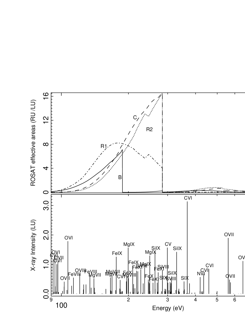
Figure 1: Top panel: Wisconsin B (plain) and C (dashed), and ROSAT R1 (dash-dotted) and R2 (dotted) band effective areas. Bottom panel: Example of calculated SWCX spectra in Line Units (photons cm^-2 s^-1 sr^-1). The emitting ions are marked above the most prominent lines.

The collision rate per volume unit R${}_{X^{\,Q+}}$ (cm^-3 s^-1) of X${}^{\,Q+}$ ions with the neutral heliospheric atoms is given by the equation:

$$R_{X^{\,Q+}}(r) = N_{X^{Q+}}(r)\,\upsilon_{r}\,(\sigma_{(H,X^{\,Q+})}\,n_{H}(r)+\,\sigma_{(He,X^{Q+})}\,n_{He}(r))$$

$$= R_{(X^{\,Q+},H)}(r)+R_{(X^{\,Q+},He)}(r)$$

where $\sigma_{(H,X^{\,Q+})}$ and $\sigma_{(He,X^{\,Q+})}$ are the hydrogen and helium CX cross-sections, n_H(r) and n_He(r) are the hydrogen and helium density distributions respectively, $\bar{\upsilon}_{r}=\bar{V}_{SW}-\bar{\upsilon}_{n}\approx\bar{V}_{SW}$ the relative velocity between SW ions and IS neutrals in the inner heliosphere, and $N_{X^{Q+}}(r)$ is the self-consistent solution to the differential equation:

$$\frac{dN_{X^{\,Q+}}}{dx}\, =\, -\,N_{X^{\,Q+}}\,(\sigma_{(H,X^{\,Q+})}\,n_{H}(x)+\,\sigma_{(He,X^{\,Q+})}\,n_{He}(x))$$

$$+\,N_{X^{\,(Q+1)+}}\,(\sigma_{(H,X^{\,(Q+1)+})}\,n_{H}(x)+\,\sigma_{(He,X^{\,(Q+1)+})}\,n_{He}(x))$$

expressing the evolution of the density distribution of ion X^Q+ along SW streamlines due to production (from CX reactions of ion X^(Q+1)+) and loss terms.

Cross-section uncertainties are mainly due to instrumental systematic errors and most important to the collision energy dependance of cross-sections. Detailed uncertainties for individual ions are not given in literature, but average uncertainties of $\sim$30% at most are reported (Wargelin et al., 2008).

Then, we establish emissivity grids in units of (photons cm^-3 s^-1):

$$\varepsilon_{i}(r)\,=R_{(X^{Q+},H)}(r)\,Y_{(E_{i},H)}+R_{(X^{Q+},He)}(r)\,Y_{(E_{i},He)}$$ (4)

where Y${}_{(E_{i},M)}$ is the photon emission yield (in number of photons) computed for a spectral line of photon energy E_i following CX with the corresponding neutral species M (H or He individually). For any line of sight (LOS) and observation date, the directional intensity of this spectral line is given by:

$$I_{E_{i}}\,(LU)=\frac{1}{4\pi}\,\int_{0}^{\,\sim 100AU}\varepsilon_{i}(s)\,ds$$ (5)

which defines the average intensity, in Line Units (LU = photons cm^-2 s^-1 sr^-1), of the spectral line for the particular date and LOS, as well as the solar cycle phase (minimum or maximum) corresponding at this date. The intensity is somewhat underestimated because of the SW ion propagation in the heliosheath up to the heliopause, and in the heliotail up to $\sim$3 000 AU, where all ions are used up. The outer heliospheric region is neglected in our model, but estimates yield a maximum additional $\sim$20% contribution in the downwind direction, with possible effects on the SWCX spectral hardness (see §4).

Our original atomic database (Kharchenko, 2005) included C^5,6+, N^5,6,7+, O^6,7,8+, Ne^8,9+ and Mg^10,11+ ions. Exact calculations of the cascading photon spectra were performed individually for these ions when they charge exchange with hydrogen and helium respectively. Detailed CX collision cross sections taking into account both the neutral target species and the solar wind velocity regime were include in the calculations (P. Stancil private communication). These calculations have already been used to reproduce observed SWCX spectra from comets with CHIPS (Sasseen et al., 2006).

The database was recently updated to include Fe^7…13+, Si^5…10+, S^6…11+, Mg^4…9+ ions that emit intense lines in the 0.1-0.3 keV range. Individual emission spectra induced in the charge exchange collisions of these ions have very complicated structures because of a large number of intermediate multiplets related to different excited states of many-electron ions. The photon yields Y(E,M) for heavier ions were calculated using the simplified hydrogenic model (Kharchenko & Dalgarno, 2000), which assumes a hydrogenic nature of electronic excited states. In this model, the effective charge of hydrogenic ion is computed from an accurate value of the ion ionization potential and branching ratios of radiative cascading transitions are chosen to be the same as in all H-like ions. Moreover, photon yields were calculated using a single neutral species, which means that no distinction between H and He was made. The hydrogenic approximation of the CX emission spectra is a quantum mechanical model in which an actual ion spectra may be replaced with the hydrogenic spectra. In this model the total energy of emitted photons is defined by an initial state-population and should be an accurate quantity matching real spectra. Positions of emission lines do not correspond exactly to real emission spectra, but this defect is not very important at the low resolution of the observed spectra. Total cross sections of CX collisions for the hydrogenic approximations have been calculated using the over-barrier model (Kharchenko & Dalgarno, 2001). An example of calculated spectra is presented in figure 1-lower panel, with the emitting ion identifying the most intense lines.

2.2 Hot Gas thermal emission

We use a Raymond-Smith (RS) hot plasma model (Raymond & Smith, 1977) assuming typical metal abundances [He, C, N, O, Ne, Mg, Si, S, Ar, Ca, Fe, Ni] = [10.93, 8.52, 7.96, 8.82, 7.96, 7.52, 7.60, 7.20, 6.90, 6.30, 7.60, 6.30] (Allen, 1973). We use this model rather than the APEC model (Smith et al., 2001) that superseded it because we are most interested in the $1\over 4$ keV range. APEC includes only transitions for which accurate atomic rates are available, while the code of Raymond and Smith estimates the emission in the large number of weak lines that are known to be present (e.g., from moderately ionized species of Mg, Si, S and Fe) but which lack accurate excitation rates and wavelengths. Given the low spectral resolution of the observations considered here and our interest in the total emitted power, the RS model serves very well.

This model gives us X-ray emissivities f₁(T) and f₂(T) convolved by and summed in the ROSAT R1 and R2 bands, respectively, as a function of temperature such that the total hot gas X-ray flux in these bands is defined as:

$$I_{12,LB}=I_{1,LB}+I_{2,LB}=EM(i,T)\cdot(f_{1}(T)+f_{2}(T))$$ (6)

where EM(i, T) is the emission measure for temperature T and look direction $i$. Units of functions f₁ and f₂ are RU EM^-1, where RU = 10^-6 cts s^-1 arcmin^-2 is the usual ROSAT detector unit and EM is the typical emission measure unit cm^-6 pc.

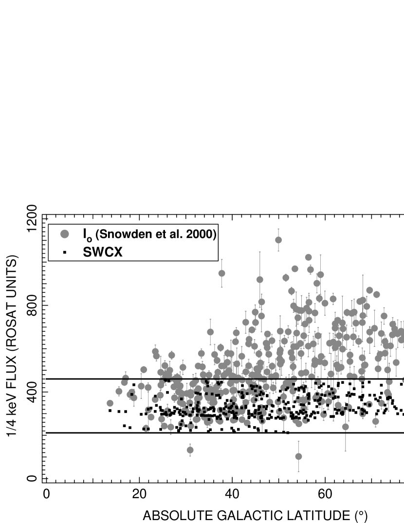
Figure 2: Measured unabsorbed (I_12,obs, from Snowden et al. (2000), gray circles) and calculated SWCX (black dots) fluxes in the ROSAT $1\over 4$ keV (R1+R2) band as a function of absolute galactic latitude for 378 shadowing observations. Flux is given in ROSAT Units (10^-6 cts s^-1 arcmin^-2).

Equivalently, the hot gas emission in bands B and C is defined as:

$$I_{B\,C,LB}=I_{B,LB}+I_{C,LB}=EM(i,T)\cdot(f_{B}(T)+f_{C}(T))$$ (7)

where f_B(T) and f_C(T) are the equivalent emissivity functions in the B and C bands derived by the RS plasma code, in units of cts s^-1 EM^-1.

3 R1+R2 intensities

We have calculated SWCX spectra in ROSAT observation geometry for the shadow field lines of sight (LOS) listed in table 1 of Snowden et al. (2000), that were observed during the ROSAT all-sky survey. The shadows analysed by Snowden et al. (2000) were located at high galactic latitudes and in general above 15^∘ from the galactic plane. The ROSAT observation geometry is defined with the view direction perpendicular to the Sun-satellite direction. Thus, it takes a six-month period to build a full-sky map of the soft X-ray intensity. The ROSAT all-sky survey was performed between July 1990 and February 1991, which corresponds to maximum solar activity conditions that were taken into account in the SWCX simulations.

Maximum solar activity conditions imply the following input parameters in the SWCX model. We consider a radiation pressure to gravity ratio $\mu$ = 1.5 for neutral hydrogen and slightly anisotropic ionization rates varying between 8.4$\times$10^-7 s^-1 at the solar equator and 6.7$\times$10^-7 s^-1 at the poles (Quémerais et al., 2006). For neutral helium, the average lifetime (inverse ionization rate) at 1 AU is 0.62$\times$10⁷ s at solar maximum, in agreement with McMullin et al. (2004). In solar maximum, the solar wind is considered to be a complex mix of slow and fast wind states that is in general approximated with an average slow wind flux. Slow solar wind flows at $\sim$ 400 km/s and has a proton density of $\sim$ 6.5 cm^-3 at the Earth position. The oxygen content with respect to protons is [O/H] = 1/1780. The most important heavy ion charge state abundances with respect to oxygen [X^q+/ O] are: C^5,6+: [0.21, 0.318], O^6,7,8+: [0.73, 0.2, 0.07], Si^8,9,10+: [0.057, 0.049, 0.021] and Fe^8,9,10,11+: [0.034, 0.041, 0.031, 0.023] (adopted from Schwadron & Cravens, 2000).

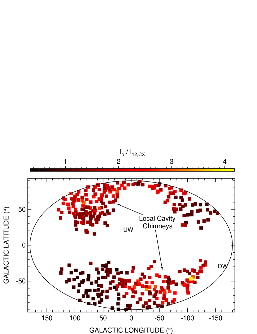
Figure 3: Unabsorbed I_12,obs R12 flux data over simulated I_12,CX SWCX flux ratio map in galactic coordinates with an equal-area Aitoff projection. For information we note the UW and DW directions in the sky. The LC chimneys appear clearly where the I_12,obs/I_12,CX ratio is the highest.

We have convolved the individual spectra with the ROSAT R1 and R2 band responses in order to calculate the total SWCX flux in these bands, as well as the total R12 (R1+R2) flux. We plot the resulting R12 SWCX flux and the unabsorbed I_12,obs component from the Snowden et al. (2000) analysis as a function of absolute galactic latitude in figure 2. I_12,obs corresponds to the unabsorbed portion of the SXRB that was originally attributed to the LB $\sim$10⁶ K hot gas. X-ray intensities are presented in ROSAT Units (RU = 10^-6 cts s^-1 arcmin^-2).

The SWCX R12 flux (black dots) varies between 212 and 460 RU with an average value of 332 RU and is fairly uniformly distributed across all latitudes. The lower and upper limits calculated in the SWCX simulations for average maximum conditions are represented with the plain black horizontal lines.

On the other hand, the unabsorbed I_12,obs component (gray circles) derived in the Snowden et al. (2000) analysis has a clear correlation with the absolute galactic latitude. Higher I_12,obs values are measured towards higher latitudes, where the local cavity is enlarged and communicates with the galactic halo through the chimneys.

In the figure it is clear that the SWCX intensity is of the same order as the I_12,obs intensity measured in low galactic latitudes (up to around 20-25^∘). We can conclude, then, that the SWCX $1\over 4$ keV flux could account for most of the observed ROSAT emission in the galactic plane. This conclusion implicitly assumes that the highly peaked exospheric SWCX contribution has been cleaned from the ROSAT data, but not the heliospheric contribution.

Fig 3 is a map in galactic coordinates of the ratio between the unabsorbed ROSAT emission and the computed SWCX contribution. The map clearly reveals the emission from the so-called chimneys that connect the Local Cavity to the northern and the southern halo. Our intensity results do not preclude that outside these chimneys the totality of the signal is SWCX emission.

4 Band ratios

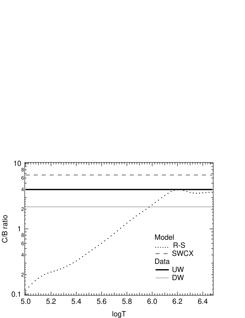
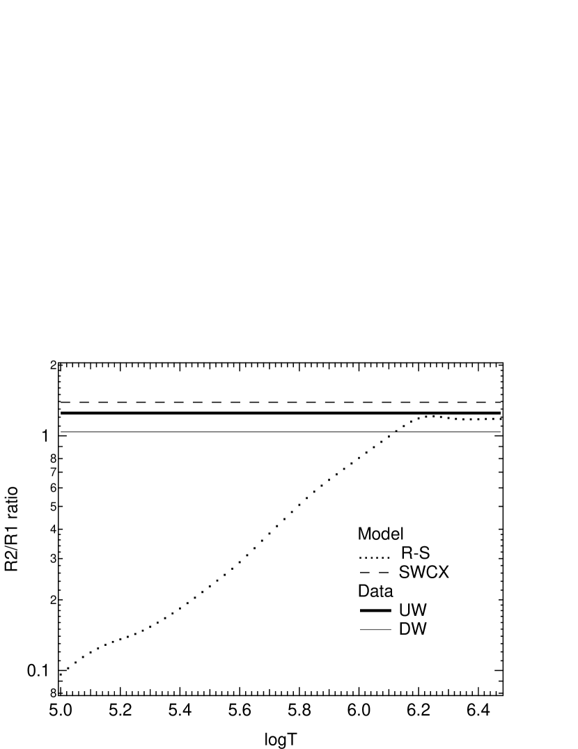
Figure 4: Wisconsin (upper panel) and ROSAT (lower panel) band ratios for data (UW-bold, DW-plain line), SWCX model (dashed line) and the R-S hot gas model (dotted line) as a function of temperature.

For each SWCX spectrum calculated in the look directions presented in figure 2 we have calculated the R2/R1 (ROSAT) and C/B (Wisconsin) ratios. We find an average R2/R1 (hereafter R_CX) ratio of 1.39 and an average C/B ratio of 6.67. Although both ratios show very little variation across the sky, there is a hardness trend of the SWCX spectra with harder spectra towards the downwind direction (UW to DW variations: R_CX = [1.36 - 1.41], C/B = [6.25 - 7.14]). However, we need to alert the reader that these are somewhat uncertain SWCX spectra and therefore somewhat uncertain band ratios. Indeed, as we mentioned in section 2, exact calculations for Fe, Si, Mg, Al are not yet available, and no distinction was done between the neutral targets (H or He), while laboratory experiments show that the energy levels populated after the electron capture and the subsequent radiative cascades may differ significantly for different targets. Since most of the SWCX downwind emission is due to the interaction with neutral helium, while on the upwind side hydrogen is the main contributor, more precise calculations could have an effect on the hardness. Also, although preliminary calculations show an almost negligible effect, the heliospheric model cutoff (especially in the DW directions) may be responsible for the “loss” of relatively more emission from lower charge states (at relatively lower energies) than emission from higher charge states (at relatively higher energies). Thus, the calculated SWCX spectra may actually be softer than what is predicted here. It is evident that a more detailed calculation taking into account all metals and the neutral target nature, as well as detailed cascading collisions (secondary ion production) in the outer heliosphere is needed in the future. On the other hand, the interval we find for the ratio can be used a reliable value for the average SWCX ratio.

These SWCX ratios have to be compared with the corresponding ratios for thermal emission. The latter were obtained as a function of temperature by convolving the Raymond-Smith spectra with the ROSAT band responses R1 and R2 and Wisconsin B and C responses. The results are shown in figure 4. Above logT= 6.1 the thermal R2/R1 ratio reaches its maximal value of $\simeq$ 1.2. It remains however slightly lower than the SWCX ratio of 1.36-1.41. At those temperatures the thermal C/B ratio increases to its maximal value of $\simeq$ 4, a value almost half the SWCX ratio of 6.24-7.14, i.e. a significant difference. Those curves allow estimates of the ratios for combinations of thermal plus SWCX background emissions.

5 Combination of the heliospheric SWCX and LB hot plasma emission

For a comparison with the data we consider two regions: one centered on the direction of the incoming IS flow at ecliptic coordinates ($\lambda$, $\beta$) $\sim$ (252.3, 8.5)^∘ for the IS H flow, according to Lallement et al. (2005) (upwind -UW- direction) and one looking at the outgoing flow direction (downwind -DW- direction). In galactic coordinates the UW direction corresponds to (l, b) = (5.4, 18.9)^∘, close to the galactic center direction (anti-galactic direction for DW respectively). These two regions are also very close to the minimum and maximum values of the hardness ratio derived by Snowden et al. (1990b), which define the so-called color gradient axis of the soft X-ray background. For these two regions we can derive average values of observed unabsorbed $1\over 4$ keV emission using the Local Bubble contours in the Snowden et al. (1998) analysis. For the upwind (UW) direction the ROSAT unabsorbed I_12,obs emission we estimate $\sim$325 RU, while for the downwind (DW) direction the observed unabsorbed level is found to be 450 RU.

The equivalent B+C intensities in the Wisconsin survey are estimated on average $\sim$90 cts s^-1 and $\sim$125 cts s^-1 for the UW and DW directions respectively (Snowden et al., 1990b). However, those intensities include both the foreground (assumed LB) and more distant components (galactic halo and extragalactic), since the Wisconsin survey did not have enough spatial resolution to study the shadowing fields. Moreover, the Wisconsin sounding rocket measurements looked in the roughly anti-Sunward direction, which should also affect the comparison with the ROSAT All-Sky Survey in terms of the SWCX component spatial distribution. For instance, for the DW look directions, the Wisconsin sounding rockets were observing directly through the He cone and should have had a higher “contamination” of SWCX emission than the ROSAT detectors that must have been located in crosswind positions on the Earth’s orbit in order to observe in the DW directions.

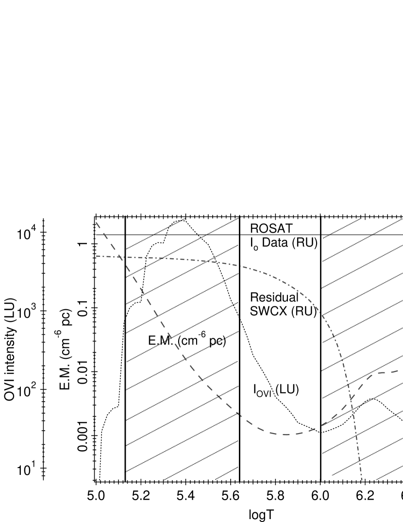
Figure 5: Solutions for the EM (dashed line) and residual SWCX emission (dot-dashed line) as a function of temperature of a hot plasma for observed R12 intensities (I_12,obs, plain horizontal lines) for an upwind (left panel) and downwind (right panel) look directions. Upper O VI doublet intensity limit (dotted line) is calculated for the EM values. Discontinuities in the O VI intensity curve are due to O VI density interpolation in the Chianti database. The cross-hatched regions show the hot gas temperature ranges excluded by O VI intensity (Shelton, 2003) and SWCX emission constraints.

The measured R2/R1 and C/B ratios for these regions are shown superimposed to the models in figure 4 and listed in Table 1. For the UW area the measured R2/R1 ratio is close to the SWCX value, although slightly smaller, while for the DW area it is significantly smaller. For both areas the measured C/B ratio is lower than the SWCX ratio. Fig 4 shows that for both areas a combination of SWCX and thermal emissions may in principle account for the ROSAT measurements, the thermal emission lowering the R2/R1 ratio to achieve the observed value. Similarly, independently of the R2/R1 ratio, fig 4 also shows that a combination of both backgrounds may account for the Wisconsin data, the thermal emission decreasing the C/B ratio to achieve the observed value.

It remains to find a combination satisfying both ratios simultaneously. Our attempt to find a solution is the following one. For each assumed temperature of the hot gas, we use the R1 and R2 data (and thus the observed ratio) and the SWCX spectral shape to derive the respective contributions of SWCX and thermal emission, i.e., we derive which quantity of SWCX induced R12 intensity and which emission measure EM for the hot gas lead to the measured intensities and the measured R2/R1 ratio. We a posteriori calculate the B and C intensities, C/B ratio and the O VI emission of the hot gas and compare with the data.

The SWCX model predicts a total R12 intensity:

$$I_{12,CX}=I_{1,CX}+I_{2,CX} = I_{1,CX}\cdot(1+R_{CX})$$ (8)

$$= I_{2,CX}\cdot\frac{1+R_{CX}}{R_{CX}}$$ (9)

where R_CX is the R2/R1 ratio predicted by the SWCX model.

The total unabsorbed flux I_12,obs(i) measured in the R12 band towards look direction $i$ is the sum of LB hot gas I_12,LB and SWCX I_12,CX fluxes: I_12,obs(i) = I_12,CX + I_12,LB, so that SWCX intensity can be written:

$$I_{12,CX}=I_{12,obs}(i)-I_{12,LB}=I_{12,obs}(i)-EM\cdot(f_{1}(T)+f_{2}(T))$$ (10)

The observed R2/R1 ratio (hereafter R_obs) towards look direction $i$ is defined by the equation:

$$R_{obs}(i)=\frac{I_{2,CX}+I_{2,LB}}{I_{1,CX}+I_{1,LB}}$$ (11)

Resolving equation 11 by using equations 6 to 10, we find the hot gas emission measure EM(i, T) as a function of temperature, total R12 measured intensity I_12,obs(i) and measured R_obs(i) ratio towards look direction $i$.

$$EM(i,T)\,=\frac{R_{CX}\,-\,R_{obs}(i)}{(R_{obs}(i)\,+\,1)\,\cdot\,(R_{CX}\cdot f_{1}(T)\,-\,f_{2}(T)\,)}\cdot I_{12,obs}(i)$$ (12)

We calculate the emission measure for the two UW and DW directions defined above using the following numerical values: (i) the R_CX ratio is constant and equal to 1.39, (ii) observed values of the unabsorbed portion of the $1\over 4$ keV emission in the R12 band are I_12,obs(UW, DW) = (325, 450) RU as derived from the LB contours in the Snowden et al. (1998) analysis for the UW and DW (respectively galactic and anti-galactic) directions, and (iii) the corresponding observed R2/R1 ratio is R_obs = 1.25 and 1.04 for the UW and DW directions respectively.

Table 1: Temperature (logT) limits and E.M. solutions for upwind (UW) and downwind (DW) look directions when combining a SWCX and RS hot plasma code. In the lower part of the table we include the observational input considered.

	Local Bubble						SWCX				(LB + SWCX)
Look	logT	E M	I12,LB	IB	IC		I12,CX	IB	IC		IBC	C/B
Direction		(10-4 cm-6 pc)	(RU)	(cts s-1)			(RU)	(cts s-1)			(cts s-1)
UW	5.64	5.5	25	3.8	2.6		300	10.	66.5		82.9	5.
DW		21.	96	14.5	10.		354	11.8	78.8		115.1	3.37
UW	6.00	3.7	62	4.8	11.1		263	9.2	58.		82.7	5.
DW		14.1	238	18.3	42.5		212	7.7	46.5		114.1	3.57
	Observational Input
	I12,obs(RU)	R2/R1 (Robs)	IBC (cts s-1)	C/B
UW	325	1.25	$\sim$ 90	4.
DW	450	1.04	$\sim$ 125	2.17

In figure 5 we show the resulting EM and the portion of the total emission due to the SWCX mechanism (called residual emission) as derived from equations 12 and 10 respectively as a function of logT and for the two look lines. We show superimposed the R12 measured intensities in those directions. For the calculated EM and corresponding temperatures we have also added to figure 5 the intensity of the O VI doublet at $\bar{\lambda}$ = 1034 Å (1032 Å and 1038 Å). In order to calculate this O VI doublet emission we have used equation (5) of Shull & Slavin (1994) and assumed that interstellar O abundance is 8.5$\times$ 10^-4. We also assume that the O VI ion proportion depends on temperature according to the Chianti database formulae for collisional equilibrium (Landi et al., 2006).

In order to delimit the possible temperature solutions for the LB hot gas, we place the following constraints: i) We assume that the SWCX model is accurate enough to ensure that the heliospheric emission in the R12 band cannot be lower than $\sim$ 212 RU (lower limit in figure 2). This gives us (from the right panel of Fig.5) an upper limit of logT = 6 in temperature. ii) We use the observed upper limit of O VI doublet intensity, reported at $\sim$ 800 LU (Shelton, 2003), which gives us two temperature limits at logT = 5.13 and 5.64 (extreme limits in the DW direction). The interval between those two temperatures is forbidden because the corresponding O VI column densities (and thus the O VI intensity) are too high to match observations. Temperatures below 10^5.13 K would predict extremely strong C VI and N VI absorption toward nearby stars, which have not been observed (e.g. Lehner et al., 2003; Welsh & Lallement, 2005) so we do not consider it a realistic solution. The limits of valid temperature intervals are marked by the vertical bold lines and the cross-hatched regions in figure 5 show the excluded temperature ranges. The two most plausible hot gas temperature limits (logT = 5.64, 6.0) along with the corresponding UW and DW emission measures and residual SWCX emission are summarized in table 1.

We also calculate for the two boundary solutions the corresponding SWCX intensities and the thermal emission intensities in the B and C bands by convolving our simulated SWCX spectra and the hot gas spectra with the band responses. For the two temperatures the total hot gas and SWCX intensity in (B + C) band is found to be about 83 cts s^-1 and about 115 cts s^-1 for the UW and DW directions respectively. This similarity arises from the similarity between the wavelength intervals covered by the B and C bands and the R1 and R2 bands (see fig. 1). The C/B ratio derived from this analysis is 5.0 and $\sim$3.5 for the UW and DW directions accordingly, for temperatures above 10^5.64 K.

The (B+C) total intensity is consistent with the lower values reported in the Wisconsin survey (Snowden et al., 1990b), which correspond to the lower galactic latitudes. Moreover, Snowden et al. (1990b) did not proceed with a shadowing analysis of the Wisconsin data, so the reported values include both local and more distant absorbed components and are expected to be higher than the hot gas and SWCX combination we present here.

However, the C/B ratio computed in the analysis (5 to $\sim$3.6 from UW to DW, depending on temperature) is inconsistent with the observed value, especially in the DW direction (observed $\sim$2.2), suggesting that we should need more hot gas emitting in the B band. This inconsistency cannot be attributed to the absorbed portion of emission included in the Wisconsin data analysis because the absorbed component is a high-T gas giving a harder spectrum since absorption is more effective in lower energies.

This inconsistency of the DW C/B ratio is important, since it seems difficult to explain in the context of our study. As a matter of fact, as can be seen in table 1, the SWCX contribution in the C band is large whatever the temperature, and reaching a C/B ratio of 2.2 requires a very small SWCX emission, in our sense far from realistic. Again, as we discussed in the introduction and it was shown in the Bellm & Vaillancourt (2005) study, the B intensity is higher than expected from the models. This seems to remain true (and even worse) when taking into account the SWCX contribution.

6 Discussion and conclusions

We have modeled the intensity and spectral characteristics of the heliospheric SWCX emission at the time of the ROSAT survey and compared with the unabsorbed, local emission derived by Snowden et al. (2000) in the $1\over 4$ keV band. The results show that the SWCX emission can account for most of the total intensity recorded in the R1+R2 bands for most of low latitude lines-of-sight. A map of the heliospheric SWCX portion of the total signal clearly reveals the high latitude chimneys to the halo as the only regions unambiguously dominated by hot gas emission. Such a result can be interpreted as meaning that little or no hot gas exists within the galactic disk.

The spectral characteristics however reveal more complexity and preclude such a simple scenario. The SWCX band ratios disagree with the observations, especially towards the galactic anti-center and at low energies (C/B). We have thus searched for a combination of SWCX and thermal emission from hot gas in equilibrium and solar abundances able to reproduce the data. Our study shows that a combination of SWCX and thermal emission can reproduce the data in the galactic center hemisphere at low latitudes. For this solution the SWCX emission strongly dominates. The temperature of the hot gas is constrained within the interval 10^5.64-10⁶. The upper limit is constrained by the lower limit on the SWCX intensity. This upper limit can be considered as firmly determined, thanks to recent observational studies above 0.3 keV that have confirmed the validity of our model (Koutroumpa et al., 2007). The temperatures lower than 10^5.64 are excluded by O VI emission observations (Shelton, 2003) and interstellar ion absorption lines toward nearby stars.

On the other hand, it is difficult to fit with such a combination the Wisconsin data. In the UW (galactic center direction) a combination of hot gas and SWCX emission gives (B+C) intensities as well as C/B ratios roughly compatible with the observed values for several different temperature ranges. The main difficulty is the impossibility to account for the very low C/B ratio measured towards the galactic anti-center direction with the present input models used in our study. We note that the high B intensity is also clearly a problem for any hot gas solution, including the very high depletion hypothesis, as shown by the study of Bellm & Vaillancourt (2005). The SWCX contribution, which hardens the spectra, reinforces this difficulty.

However, further investigation is required on the model’s uncertainties in order to quantify their influence on the spectral hardness of SWCX emission. Further analysis of the hydrogenic ion approximation is needed, since hydrogenic ions tend to emit photons at higher energies following CX (since high-n to ground transitions are generally allowed) than the multi-electron ions considered here (because selection rules and more complicated atomic structure lead to more cascades before the final transition to ground. Therefore, it is likely that the model spectra have significantly less flux at low energies than they should. Given the steeply decreasing effective areas at lower energies (see Fig. 1), this would help explain some of the discrepancies seen in the C/B ratio. Also, the fact that no distinction was made between the neutral targets (H or He) in the $1\over 4$ keV calculations, would also have an effect on the spectral hardness, since there is an effect on the electron capture level (roughly proportional to $\sqrt{13.6\,eV/I_{n}}$, where $I_{n}$ is the neutral target ionization potential), the capture level with He being somewhat lower than with H. The ROSAT observation geometry tends to smooth out those differences, but the SWCX spectrum will tend to be softer in the DW directions (i.e., looking through or near the He cone), again helping to explain some of the C/B ratio anomaly. Finally, at the low energies of the B band, more detailed calculations of the heliospheric and magnetospheric signals must be performed, especially the low energy secondary SWCX emissions in the heliosheath and heliotail, i.e. subsequent recombinations of partially neutralized solar wind high ions.

References

- Allen (1973) Allen, C. W. 1973, London: University of London, Athlone Press, —c1973, 3rd ed.
- Bellm & Vaillancourt (2005) Bellm, E. C., & Vaillancourt, J. E. 2005, ApJ, 622, 959
- Bhardwaj et al. (2007) Bhardwaj, A., et al. 2007, Planet. Space Sci., 55, 1135
- Bloch et al. (1986) Bloch, J. J., Jahoda, K., Juda, M., McCammon, D., Sanders, W. T., & Snowden, S. L. 1986, ApJ, 308, L59
- Bowyer et al. (1968) Bowyer, C. S., Field, G. B., & Mack, J. F. 1968, Nature, 217, 32
- Bregman & Lloyd-Davies (2006) Bregman, J. N., & Lloyd-Davies, E. J. 2006, ApJ, 644, 167
- Burrows & Mendenhall (1991) Burrows, D. N., & Mendenhall, J. A. 1991, Nature, 351, 629
- Cox (1998) Cox, D. P. 1998, Lecture Notes in Physics, Berlin Springer Verlag, 506, 121
- Cravens (1997) Cravens, T. E., 1996, Geophys. Res. Lett., 24, 105
- Cravens (2000) Cravens, T. E. 2000, ApJ, 532, L153
- Cravens et al. (2001) Cravens, T. E., Robertson, I. P., & Snowden, S. L. 2001, J. Geophys. Res., 106, 24883
- Frisch & York (1983) Frisch, P. C., & York, D. G. 1983, ApJ, 271, L59
- Hasinger et al. (1993) Hasinger, G., Burg, R., Giacconi, R., Hartner, G., Schmidt, M., Trumper, J., & Zamorani, G. 1993, A&A, 275, 1
- Henley & Shelton (2008) Henley, D. B., Shelton, R. L. 2008, ApJ, 676, 335
- Herbstmeier et al. (1995) Herbstmeier, U., Mebold, U., Snowden, S. L., Hartmann, D., Butler Burton, W., Moritz, P., Kalberla, P. M. W., & Egger, R. 1995, A&A, 298, 606
- Hurwitz et al. (2005) Hurwitz, M., Sasseen, T. P., & Sirk, M. M. 2005, ApJ, 623, 911
- Indebetouw & Shull (2004) Indebetouw, R., & Shull, J. M. 2004, ApJ, 607, 309
- Jelinsky et al. (1995) Jelinsky, P., Vallerga, J. V., & Edelstein, J. 1995, ApJ, 442, 653
- Jenkins (2002) Jenkins, E. B. 2002, ApJ, 580, 938
- Kharchenko (2005) Kharchenko, V. 2005, AIPC, 774, 271
- Kharchenko & Dalgarno (2000) Kharchenko, V., & Dalgarno, A. 2000, J. Geophys. Res., 105, 1854
- Kharchenko & Dalgarno (2001) Kharchenko, V., & Dalgarno, A. 2001, ApJ, 554, L99
- Koutroumpa et al. (2007) Koutroumpa, D., Acero, F., Lallement, R., Ballet, J., Kharchenko, V. 2007, A&A, 475, 901
- Koutroumpa et al. (2008) Koutroumpa, D., Lallement, R., Kharchenko, V., & Dalgarno, A. 2008, Space Science Reviews, 87
- Koutroumpa et al. (2006) Koutroumpa, D., Lallement, R., Kharchenko, V., Dalgarno, A., Pepino, R., Izmodenov, V., Quémerais, E. 2006, A&A, 460, 289
- Lallement (1998) Lallement, R. 1998, IAU Colloq. 166: The Local Bubble and Beyond, 506, 19
- Lallement (2004) Lallement, R. 2004, A&A, 422, 391
- Lallement et al. (2005) Lallement, R., Quémerais, E., Bertaux, J. L., Ferron, S., Koutroumpa, D., Pellinen, R. 2005, Science, 307, 1447
- Lallement et al. (2003) Lallement, R., Welsh, B. Y., Vergely, J. L., Crifo, F., & Sfeir, D. 2003, A&A, 411, 447
- Landi et al. (2006) Landi, E., Del Zanna, G., Young, P. R., Dere, K. P., Mason, H. E., & Landini, M. 2006, ApJS, 162, 261
- Lehner et al. (2003) Lehner, N., Jenkins, E. B., Gry, C., Moos, H. W., Chayer, P., & Lacour, S. 2003, ApJ, 595, 858
- Lisse et al. (1996) Lisse, C. M., Dennerl, K., Englhauser, J., Harden, M., Marshall, F. E., Mumma, M. J., Petre, R., Pye, J. P., Ricketts, M. J., Schmitt, J., Trumper, J., West, R. G. 1996, Science, 274, 205
- McCammon et al. (1983) McCammon, D., Burrows, D. N., Sanders, W. T., & Kraushaar, W. L. 1983, ApJ, 269, 107
- McMullin et al. (2004) McMullin, D. R., Bzowski, M., Möbius, E., Pauluhn, A., Skoug, R., Thompson, W. T., Witte, M., von Steiger, R., Rucinski, D., Judge, D., Banaszkiewicz, M., Lallement, R. 2004, A&A, 426, 885
- Pepino et al. (2004) Pepino, R., Kharchenko, V., Dalgarno, A., & Lallement, R. 2004, ApJ, 617, 1347
- Quémerais et al. (2006) Quémerais, E., Lallement, R., Ferron, S., Koutroumpa, D., Bertaux, J.-L., Kyrölä, E., Schmidt, W. 2006, J. Geophys. Res., 111, A10, 9114-+
- Raymond & Smith (1977) Raymond, J. C., Smith, B.W. 1977, ApJS, 35, 419
- Robertson et al. (2006) Robertson, I. P., Collier, M. R., Cravens, T. E., & Fok, M.-C. 2006, Journal of Geophysical Research (Space Physics), 111, 12105
- Robertson & Cravens (2003) Robertson, I. P., & Cravens, T. E. 2003, Geophys. Res. Lett., 30(8), 1439
- Sanders et al. (1977) Sanders, W. T., Kraushaar, W. L., Nousek, J. A., & Fried, P. M. 1977, ApJ, 217, L87
- Sasseen et al. (2006) Sasseen, T. P., Hurwitz, M., Lisse, C. M., Kharchenko, V., Christian, D., Wolk, S. J., Sirk, M. M., & Dalgarno, A. 2006, ApJ, 650, 461
- Schwadron & Cravens (2000) Schwadron, N. A., Cravens, T. E. 2000, ApJ, 544, 558
- Shelton (2003) Shelton, R. L. 2003, ApJ, 589, 261
- Shull & Slavin (1994) Shull, J. M., & Slavin, J. D. 1994, ApJ, 427, 784
- Slavin & Frisch (2002) Slavin, J. D., & Frisch, P. C. 2002, ApJ, 565, 364
- Smith et al. (2001) Smith, R. K., Brickhouse, N. S., Liedahl, D. A., & Raymond, J. C. 2001, ApJ, 59, 141
- Smith et al. (2007) Smith, R. K., et al. 2007, PASJ, 556, L91
- Snowden et al. (2004) Snowden, S. L., Collier, M. R., Kuntz, K. D. 2004, ApJ, 610, 1182
- Snowden et al. (1990a) Snowden, S. L., Cox, D. P., McCammon, D., & Sanders, W. T. 1990, ApJ, 354, 211
- Snowden et al. (1998) Snowden, S. L., Egger, R., Finkbeiner, D. P., Freyberg, M. J., Plucinsky, P. P. 1998, ApJ, 493,715
- Snowden et al. (2000) Snowden, S. L., Freyberg, M. J., Kuntz, K. D., Sanders, W. T. 2000, ApJS, 128, 171
- Snowden et al. (1994) Snowden, S. L., Hasinger, G., Jahoda, K., Lockman, F. J., McCammon, D., & Sanders, W. T. 1994, ApJ, 430, 601
- Snowden et al. (1994) Snowden, S. L., McCammon, D., Burrows, D. N., Mendenhall, J. A. 1994, ApJ, 424, 714
- Snowden et al. (1990b) Snowden, S. L., Schmitt, J. H. M. M., Edwards, B. C. 1990, ApJ, 364, 118
- Wargelin et al. (2008) Wargelin, B. J., Beiersdorfer, P., Brown, G. V. 2008, CaJPh, 86, 151
- Welsh et al. (1998) Welsh, B. Y., Crifo, F., & Lallement, R. 1998, A&A, 333, 101
- Welsh & Lallement (2005) Welsh, B. Y., & Lallement, R. 2005, A&A, 436, 615
- Welsh & Lallement (2008) Welsh, B. Y., & Lallement, R. 2008, A&A, in press
- Williamson et al. (1974) Williamson, F. O., Sanders, W. T., Kraushaar, W. L., McCammon, D., Borken, R., & Bunner, A. N. 1974, ApJ, 193, L133