Interfacial instability induced by lateral vapor pressure fluctuation in bounded thin liquid-vapor layers

Abstract

We study an instability of thin liquid-vapor layers bounded by rigid parallel walls from both below and above. In this system, the interfacial instability is induced by lateral vapor pressure fluctuation, which is in turn attributed to the effect of phase change: evaporation occurs at a hotter portion of the interface and condensation at a colder one. The high vapor pressure pushes the interface downward and the low one pulls it upward. A set of equations describing the temporal evolution of the interface of the liquid-vapor layers is derived. This model neglects the effect of mass loss or gain at the interface and guarantees the mass conservation of the liquid layer. The result of linear stability analysis of the model shows that the presence of the pressure dependence of the local saturation temperature mitigates the growth of long-wave disturbances. The thinner vapor layer enhances the vapor pressure effect. We find the stability criterion, which suggests that only slight temperature gradients are sufficient to overcome the gravitational effect for a water/vapor system. The same holds for the Rayleigh-Taylor unstable case, with a possibility that the vapor pressure effect may be weakened if the accommodation coefficient is below a certain critical value.

I Introduction

Thin liquid films have been intensively studied over the last decades. Many contributions have been devoted to them, owing to their technological importance and wide industrial applications. Their rich interfacial behaviors originate from combinations of various effects such as capillarity, intermolecular forces, thermocapillarity and gravity. One important effect among them is evaporation or condensation. It was often incorporated in the studies of thin films, burelbach88:_nonlin ; oron97:_long and dewetting patterns resulting from drying of films were analyzed. oron00:_three ; schwartz01:_dewet ; lyushnin02:_finger

Many past studies on evaporating or condensing liquid films have ignored the dynamics of the gas above the liquid film, assuming the infinitely deep gas phase. burelbach88:_nonlin ; oron97:_long ; bestehorn06:_regul_rayleig_taylor However, in this study we consider a situation where the gas phase is bounded by rigid parallel wall from above and has a finite depth comparable with the liquid one. The full linear stability analyses of this system were performed in several papers.huang92:_instab ; ozen04 ; ozen06:_rayleig_taylor ; mcfadden07:_onset ; mcfadden09:_onset_of_oscil_convec_in Despite the apparent simplicity of the configuration, this system includes a free surface and interfacial boundary conditions involving phase change, and therefore is very sophisticated. In order to simplify this problem, we apply long-wave approximation to both layers.

The advantage of the use of long-wave or lubrication approximation is the reduction of dimensionality: a one-dimensional (two-dimensional) film evolution equation can be derived in a two-dimensional (three-dimensional) system. Normally, only the dynamics of the liquid is considered, leading to a one-sided model. However, if the ambient gas layer is thin enough, a two-layer model would better describe the system. This was demonstrated by VanHook et al.,vanhook97:_long_benar who developed a two-layer theory to reproduce their experimental results. They showed that their two-layer model better predicts the onset of instability in their experiment than the corresponding one-layer model and also correctly describes the formation of localized elevations. In their approach, only the heat conduction in the gas phase is taken into account, and the gas dynamics is ignored because the viscosity of the gas is much less than that of the liquid. Later, Merkt et al.merkt05:_long presented an evolution equation of the interface of two viscous fluid layers in the same geometry. Their model allows for the shear stress induced by the motion of the upper layer and therefore is reduced to the single layer equation in the limit of small viscosity of the upper layer. Although their goal is the observation of pattern formation in the long-time regime, the two-layer models have been applied to the cases of Rayleigh-Taylor instabilityburgess01:_suppr ; alexeev07:_suppr_rayleig_taylor_maran and ultrathin films.joo00:_inter ; lenz07:_compet

Nevertheless, in the two-layer systems mentioned above there is no phase transformation at the interface. Here, we construct a two-layer theory for liquid-vapor layers which undergo phase change, using long-wave approximation. Note that the application of long-wave theory to the vapor phase was made in the study of film boiling.panzarella00:_nonlin If we take into account the effect of the mass flux across the interface, an instability peculiar to this system is expected, even for the presence of large disparity in viscosity and density between liquid and vapor; see Fig. 1. The liquid film is initially in equilibrium with its vapor layer. If the liquid side is heated or the vapor side is cooled, evaporation occurs at a hotter portion of the interface and condensation at a colder one. Since the vapor layer is bounded, the vapor pressure becomes higher in the evaporating region and lower in the condensing one. According to this lateral vapor pressure gradient, the higher vapor pressure pushes the interface downward and the lower one pulls it upward. Then, the surface deflection is amplified. To our knowledge, this pressure-induced instability mechanism has not been considered in the past, because the uniform ambient vapor pressure has been assumed in previous studies of evaporating or condensing liquid films. burelbach88:_nonlin ; oron97:_long ; bestehorn06:_regul_rayleig_taylor

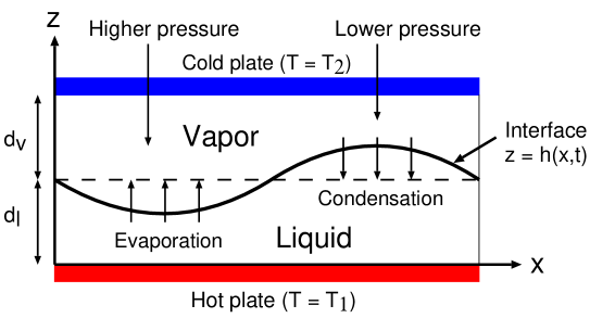
Figure 1: Instability mechanism of the present system.

To derive the model, we require the interfacial boundary conditions such that the mass transfer occurs between the phases. We follow those of the earlier studies on evaporating or condensing liquid filmsburelbach88:_nonlin ; oron97:_long except the thermodynamic relation at the interface. They used the linearized equation where the mass flux through the interface is proportional to the difference between the interfacial temperature and its saturation value corresponding to the surrounding vapor pressure, based on kinetic theory.palmer76 This relation cannot be directly applied to the present problem, because the local saturation temperature varies in the lateral direction, depending on the vapor pressure. Hence, we must modify the relation to take this effect into account. Fortunately, this can be easily done in the thermodynamic framework. For instance, Ajaev and Homsyajaev01:_stead and WaynerwaynerCSA used a nonequilibrium thermodynamic relation including the saturation temperature variation due to capillarity and disjoining pressure. This effect was later included in the model of evaporating or condensing thin liquid films.shklyaev07:_stabil However, they assumed the vapor pressure to be constant. In our two-layer model, this relation should be extended in accordance with the vapor pressure variation. Thus, one of the purposes of this work is to investigate the effect of the vapor pressure dependence of the local saturation temperature. Note that this effect was not considered in the film boiling case,panzarella00:_nonlin although the lateral vapor pressure variation, which drives the motion of the vapor, certainly exists in the boiling film. It is worthwhile noting that a somewhat similar motivation to ours is found in Ref. sultan05:_evapor, , where the vapor concentration in the ambient gas phase above the liquid film fluctuates and thereby the mass flux varies along the interface. However, they neglect the bulk gas dynamics itself and consider only the diffusion of the vapor.

Here, we start with a more general nonequilibrium thermodynamic law, which reduces to, in the linear domain, a proportional connection between the interfacial mass flux and the difference of chemical potential in each phase.colinet01:_nonlin_dynam_surfac_tension_driven_instab From this law, we can naturally derive a thermodynamic relation similar to that of Ajaev and Homsy and Wayner. Moreover, the condition of local thermodynamic equilibrium, adopted in some papers on two-phase problem,ozen04 ; onuki05:_dropl ; mcfadden07:_onset ; mcfadden09:_onset_of_oscil_convec_in is recovered by taking the appropriate limit of the derived relation. Therefore, the thermodynamic relation used here is also the extension of the interfacial equilibrium condition into nonequilibrium states. We note that more general formulation taking into account the nonequilibrium effect contains a temperature discontinuity at the liquid-vapor interface during evaporation or condensation, as was done in Ref. margerit03:_inter_benar_maran, . However, this temperature jump may be neglected unless the phase change occurs too rapidly.colinet01:_nonlin_dynam_surfac_tension_driven_instab

In the derivation of our model, we manipulate the mass flux balance equation at the liquid-vapor interface. In the literature, the effect of mass loss or gain at the liquid surface due to evaporation or condensation has been included into the model through this equation by assuming that the vapor speed is much larger than the liquid one because the vapor density is much smaller than the liquid one. burelbach88:_nonlin ; oron97:_long However, in this paper we show another interpretation of this equation as a consequence of order estimate. If we assume that the degree of the disparity in density between two phases is much greater than that in viscosity, which is valid for most substances far from the critical point, we can find that the liquid velocity is not balanced by the vapor one in the mass balance equation. Instead, it is balanced by the interface velocity, which indicates that the effect of mass loss or gain can be neglected. This order estimate leads to the approximation of the mass balance equation, where the total mass of the liquid is conserved and the effect of the mass flux affects only the dynamics of the vapor. Under this approximation, we derive the model where the conservation of the total liquid mass is guaranteed, whereas the effect of evaporation or condensation remains in the vapor dynamics.

The paper is organized as follows. The model is formulated in Sec. II, where the interfacial boundary condition and scaling peculiar to this system mentioned above are introduced. Linear stability results are presented in Sec. III, including analyses of the Rayleigh-Taylor instability and the effect of degree of nonequilibrium on it. Section IV summarizes the results and future work.

II Formulation

For simplicity we consider a two-dimensional system as in Fig. 1, where the horizontal bilayers, liquid and vapor of the same substance, are confined by rigid parallel walls from both below and above. We assume that the initial equilibrium thicknesses of the liquid and vapor layers, $d_{l}$ and $d_{v}$, are small enough to ignore the buoyancy effect. The temperatures of the liquid-side and vapor-side plates are controlled at $T_{1}$ and $T_{2}$. The x axis is taken to be parallel to the walls, and the z axis perpendicular to them. The $z=0$ plane corresponds to the boundary between the liquid and the liquid-side plate. The position of the liquid-vapor interface is described by $z=h(x,t)$. Gravity acts in the negative direction of the z axis.

II.1 Governing equations

We assume that the equations of continuity for incompressible fluids and of the momentum and energy balance hold in each phase. They are given by, respectively,

$$\nabla\cdot\mathbf{v}_{\beta} = 0,$$ (1a)

$$\rho_{\beta}(\partial_{t}\mathbf{v}_{\beta}+\mathbf{v}_{\beta}\cdot\nabla\mathbf{v}_{\beta}) = -\nabla p_{\beta}+\eta_{\beta}\nabla^{2}\mathbf{v}_{\beta}-\rho_{\beta}g\mathbf{e}_{z},$$ (1b)

$$\partial_{t}T_{\beta}+\mathbf{v}_{\beta}\cdot\nabla T_{\beta} = \kappa_{\beta}\nabla^{2}T_{\beta}.$$ (1c)

Here, $\mathbf{v}_{\beta}=(u_{\beta},w_{\beta})$, $p_{\beta}$ and $T_{\beta}$ are velocity, pressure and temperature fields, respectively, in the $\beta=\{v,l\}$ phase, where $v$ denotes the vapor and $l$ the liquid. The differential operator is $\nabla\equiv(\partial_{x},\partial_{z})$. The coefficients $\rho_{\beta}$, $\eta_{\beta}$ and $\kappa_{\beta}$ denote the density, dynamic viscosity and thermal diffusivity in the $\beta$ phase, respectively, which are assumed to be constant in each phase. In Eq. (1b), $g$ is the gravitational acceleration and $\mathbf{e}_{z}$ the unit vector in the $z$ direction.

II.2 Boundary conditions

At the walls ($z=0$ and $z=d_{l}+d_{g}$), we impose no-slip boundary conditions. Along with the temperature conditions prescribed above, they read

$$\mathbf{v}_{l}=\mathbf{0},\quad T_{l}=T_{1}\quad \quad z=0,$$ at (2a)

$$\mathbf{v}_{v}=\mathbf{0},\quad T_{v}=T_{2}\quad \quad z=d_{l}+d_{v}.$$ at (2b)

At the liquid-vapor interface $z=h(x,t)$, the mass flux $J$ must be conserved:

$$J=\rho_{v}(\mathbf{v}_{v}\cdot\mathbf{n}-\mathbf{v}_{I}\cdot\mathbf{n})=\rho_{l}(\mathbf{v}_{l}\cdot\mathbf{n}-\mathbf{v}_{I}\cdot\mathbf{n}).$$ (3)

Here, $\mathbf{n}$ is the unit normal vector directed toward the vapor,

$$\mathbf{n}=\frac{(-\partial_{x}h,1)}{\sqrt{1+(\partial_{x}h)^{2}}},$$ (4)

and $\mathbf{v}_{I}$ represents the interface velocity, which satisfies the kinematic condition

$$\mathbf{v}_{I}\cdot\mathbf{n}=\frac{\partial_{t}h}{\sqrt{1+(\partial_{x}h)^{2}}}.$$ (5)

We assume the continuity of the tangential velocity along the interface,

$$\mathbf{v}_{v}\cdot\mathbf{t}=\mathbf{v}_{l}\cdot\mathbf{t},$$ (6)

where $\mathbf{t}$ is the unit tangent vector to the interface,

$$\mathbf{t}=\frac{(1,\partial_{x}h)}{\sqrt{1+(\partial_{x}h)^{2}}}.$$ (7)

The interfacial stress and energy balance equations read, respectively,burelbach88:_nonlin ; oron97:_long

$$J(\mathbf{v}_{l}-\mathbf{v}_{v})+(p_{l}-p_{v})\mathbf{n}-(2\eta_{l}\mathbf{E}_{l}-2\eta_{v}\mathbf{E}_{v})\cdot\mathbf{n}+2\sigma H\mathbf{n}=\mathbf{0},$$ (8)

$$J\{L+\frac{1}{2}[(\mathbf{v}_{v}-\mathbf{v}_{I})\cdot\mathbf{n}]^{2}-\frac{1}{2}[(\mathbf{v}_{l}-\mathbf{v}_{I})\cdot\mathbf{n}]^{2}\}+\lambda_{l}\nabla T_{l}\cdot\mathbf{n}-\lambda_{v}\nabla T_{v}\cdot\mathbf{n}$$

$${}+[2\eta_{l}\mathbf{E}_{l}\cdot(\mathbf{v}_{l}-\mathbf{v}_{I})-2\eta_{v}\mathbf{E}_{v}\cdot(\mathbf{v}_{v}-\mathbf{v}_{I})]\cdot\mathbf{n}=0,$$ (9)

where $\mathbf{E}_{\beta}$, $\sigma$, $H$, $L$ and $\lambda_{\beta}$ are the rate-of-strain tensor in the $\beta$ phase, the surface tension, the mean curvature of the interface

$$2H=\frac{\partial_{x}^{2}h}{[1+(\partial_{x}h)^{2}]^{3/2}},$$ (10)

the latent heat and the thermal conductivity in the $\beta$ phase, respectively. In Eq. (8), we ignore the thermocapillary (Marangoni) term and assume $\sigma$ as well as $L$ and $\lambda_{\beta}$ to be constant for simplicity. The Marangoni effect on two-phase surfaces has often been neglected in the literature.huang92:_instab ; panzarella00:_nonlin ; lyushnin02:_finger ; bestehorn06:_regul_rayleig_taylor The recent investigations on the linearized systems of liquid-vapor layersozen04 ; mcfadden07:_onset ; mcfadden09:_onset_of_oscil_convec_in and drop or bubbleonuki05:_dropl , show that the Marangoni effect has little significance in pure two-phase coexisting states, because the liquid-vapor interface becomes almost isothermal owing to the large entropy difference between the two phases. In the Appendix, we include the thermocapillary term in our model and examine its effect. We numerically find that the thermocapillarity makes little contribution to linear stability of a stationary state of the model at least in the physical situations considered here. The projection of Eq. (8) on the normal and tangent to the interface yields, respectively,

$$J(\mathbf{v}_{l}-\mathbf{v}_{v})\cdot\mathbf{n}+p_{l}-p_{v}-\mathbf{n}\cdot(2\eta_{l}\mathbf{E}_{l}-2\eta_{v}\mathbf{E}_{v})\cdot\mathbf{n}+2\sigma H=0,$$ (11a)

$$\mathbf{t}\cdot(2\eta_{l}\mathbf{E}_{l}-2\eta_{v}\mathbf{E}_{v})\cdot\mathbf{n}=0,$$ (11b)

where Eq. (6) was used in the second equation. Assuming the moderate phase change rate, the continuity of the temperature at the interface holds:

$$T_{l}=T_{v}\equiv T_{I}.$$ (12)

Finally, in order to close the system we require an additional boundary condition, which relates to the interfacial thermodynamic state. In this study, we adopt the linearized phenomenological law such that the mass flux across the interface is proportional to deviation from local thermodynamic equilibrium:colinet01:_nonlin_dynam_surfac_tension_driven_instab

$$J=\hat{K}[\mu_{l}(p_{l},T_{I})-\mu_{v}(p_{v},T_{I})].$$ (13)

Here, $\mu_{\beta}$ is the chemical potential in the $\beta$ phase, which is a function of the pressure in the corresponding phase and the temperature at the interface. A proportionality coefficient $\hat{K}$ will be later specified by analogy with the kinetic theory. We now expand the chemical potentials into Taylor series in this equation around their initial equilibrium value $\mu_{0}$ with respect to the variations of the pressure and the temperature,

$$\delta p_{\beta} = p_{\beta}-p_{0},$$ (14a)

$$\delta T = T_{I}-T_{sat}(p_{0}),$$ (14b)

where $T_{sat}(p_{0})$ is the saturation temperature at the initial equilibrium pressure $p_{0}$. Using the Gibbs-Duhem relation for a one-component system, we obtain for each phase

$$\mu_{\beta}(p_{\beta},T_{I})=\mu_{0}-s_{\beta}\delta T+\frac{1}{\rho_{\beta}}\delta p_{\beta},$$ (15)

where $s_{\beta}$ is the entropy density of the $\beta$ phase. Substituting Eq. (15) into Eq. (13) yields

$$J=\hat{K}\left(\Delta s\delta T+\frac{1}{\rho_{l}}\delta p_{l}-\frac{1}{\rho_{v}}\delta p_{v}\right),$$ (16)

where $\Delta s\equiv s_{v}-s_{l}$ is the entropy difference between the phases and related to the latent heat by $L=T_{sat}(p_{0})\Delta s$. If we neglect the pressure terms on the right hand side of Eq. (16), we recover the usual kinetic relation.palmer76 ; burelbach88:_nonlin ; oron97:_long ; panzarella00:_nonlin ; bestehorn06:_regul_rayleig_taylor On the other hand, in the limit $\hat{K}\rightarrow\infty$, Eq. (16) reduces to the condition of local thermodynamic equilibrium, used in several phase-boundary problems.ozen04 ; onuki05:_dropl ; mcfadden07:_onset ; mcfadden09:_onset_of_oscil_convec_in Therefore, Eq. (16) is an intermediate relation connecting the two different interfacial conditions appearing in the studies of two-phase systems with phase change.

II.3 Dimensionless equations and parameters

In order to nondimensionalize the above equations, we scale lengths, time, velocities, pressures, temperatures and mass flux by $d_{l}$, $\displaystyle\frac{d_{l}^{2}\rho_{l}}{\eta_{l}}$, $\displaystyle\frac{\eta_{l}}{d_{l}\rho_{l}}$, $\displaystyle\frac{\eta_{l}^{2}}{d_{l}^{2}\rho_{l}}$, $\Delta T$ and $\displaystyle\frac{\lambda_{l}\Delta T}{d_{l}L}$, respectively, where $\Delta T$ is the initial temperature difference across the liquid layer. We find $\Delta T$ together with $T_{sat}(p_{0})$, solving Eq. (1c) for both phases with the boundary conditions (2), (9) and (12) in the equilibrium steady state ($J=0$), as follows:

$$\Delta T\equiv T_{1}-T_{sat}(p_{0})=\displaystyle\frac{\lambda}{\lambda+d}(T_{1}-T_{2}),$$ (17a)

$$T_{sat}(p_{0})=\displaystyle\frac{\lambda T_{2}+dT_{1}}{\lambda+d}.$$ (17b)

Here, the dimensionless parameters $\lambda$ and $d$ have been introduced. The definitions of dimensionless parameters appearing in this paper are presented in Table 1. Furthermore, we define the dimensionless pressure and temperature such that their initial equilibrium values at the interface, $p_{0}$ and $T_{sat}(p_{0})$, correspond to $0$ in their new variables. In the following, we show the resulting nondimensionalized equations.

First, the governing equations of the liquid layer (1) become

$$\nabla\cdot\mathbf{v}_{l} = 0,$$ (18a)

$$\partial_{t}\mathbf{v}_{l}+\mathbf{v}_{l}\cdot\nabla\mathbf{v}_{l} = -\nabla p_{l}+\nabla^{2}\mathbf{v}_{l}-G\mathbf{e}_{z},$$ (18b)

$$P(\partial_{t}T_{l}+\mathbf{v}_{l}\cdot\nabla T_{l}) = \nabla^{2}T_{l},$$ (18c)

and those of the vapor layer

$$\nabla\cdot\mathbf{v}_{v} = 0,$$ (19a)

$$\rho(\partial_{t}\mathbf{v}_{v}+\mathbf{v}_{v}\cdot\nabla\mathbf{v}_{v}) = -\nabla p_{v}+\eta\nabla^{2}\mathbf{v}_{v}-\rho G\mathbf{e}_{z},$$ (19b)

$$P(\partial_{t}T_{v}+\mathbf{v}_{v}\cdot\nabla T_{v}) = \kappa\nabla^{2}T_{v}.$$ (19c)

The boundary conditions at the walls (2) reduce to

$$u_{l}=w_{l}=0,\quad T_{l}=1\quad \quad z=0,$$ at (20a)

$$u_{v}=w_{v}=0,\quad\displaystyle T_{v}=-\frac{d}{\lambda}\quad \quad z=1+d,$$ at (20b)

and those at the interface (3), (5), (6), (11), (9), (12) and (16), respectively,

$$EJ=\rho(\mathbf{v}_{v}\cdot\mathbf{n}-\mathbf{v}_{I}\cdot\mathbf{n})=\mathbf{v}_{l}\cdot\mathbf{n}-\mathbf{v}_{I}\cdot\mathbf{n},$$ (21a)

$$\mathbf{v}_{I}\cdot\mathbf{n}=\displaystyle\frac{\partial_{t}h}{\sqrt{1+(\partial_{x}h)^{2}}},$$ (21b)

$$\mathbf{v}_{v}\cdot\mathbf{t}=\mathbf{v}_{l}\cdot\mathbf{t},$$ (21c)

$$EJ(\mathbf{v}_{l}-\mathbf{v}_{v})\cdot\mathbf{n}+p_{l}-p_{v}-\mathbf{n}\cdot(2\mathbf{E}_{l}-2\eta\mathbf{E}_{v})\cdot\mathbf{n}+2SH=0,$$ (21d)

$$\mathbf{t}\cdot(2\mathbf{E}_{l}-2\eta\mathbf{E}_{v})\cdot\mathbf{n}=0,$$ (21e)

$$\displaystyle J+\frac{J\Pi\Theta}{2E}\{[(\mathbf{v}_{v}-\mathbf{v}_{I})\cdot\mathbf{n}]^{2}-[(\mathbf{v}_{l}-\mathbf{v}_{I})\cdot\mathbf{n}]^{2}\}+\nabla T_{l}\cdot\mathbf{n}-\lambda\nabla T_{v}\cdot\mathbf{n}$$

$$\displaystyle{}+\frac{2\Pi\Theta}{E^{2}}[\mathbf{E}_{l}\cdot(\mathbf{v}_{l}-\mathbf{v}_{I})-\eta\mathbf{E}_{v}\cdot(\mathbf{v}_{v}-\mathbf{v}_{I})]\cdot\mathbf{n}=0,$$ (21f)

$$T_{l}=T_{v}=T_{I},$$ (21g)

$$J=K\left[T_{I}+\displaystyle\frac{\Pi}{E}\left(p_{l}-\frac{1}{\rho}p_{v}\right)\right].$$ (21h)

In Eq. (21h) we have introduced the dimensionless parameter $K$, instead of $\hat{K}$ in Eq. (16), which has the dimension. The parameters $K$ and $\hat{K}$ are related through $K=d_{l}L\hat{K}/\lambda_{l}$. The value of the parameter $K$ defined in Table 1 is determined by the comparison with the kinetic theory (Hertz-Knudsen law). In its definition, $\alpha$ is the accommodation coefficient, $m$ is the molecular mass of the fluid and $k_{B}$ is the Boltzmann constant.

Table 1: Dimensionless parameters.

Gravity	$\displaystyle G=\frac{gd_{l}^{3}\rho_{l}^{2}}{\eta_{l}^{2}}$	Density ratio	$\displaystyle\rho=\frac{\rho_{v}}{\rho_{l}}$
Liquid Prandtl number	$\displaystyle P=\frac{\eta_{l}}{\rho_{l}\kappa_{l}}$	Dynamic viscosity ratio	$\displaystyle\eta=\frac{\eta_{v}}{\eta_{l}}$
Evaporation number	$\displaystyle E=\frac{\lambda_{l}\Delta T}{\eta_{l}L}$	Conductivity ratio	$\displaystyle\lambda=\frac{\lambda_{v}}{\lambda_{l}}$
Surface tension	$\displaystyle S=\frac{\sigma\rho_{l}d_{l}}{\eta_{l}^{2}}$	Diffusivity ratio	$\displaystyle\kappa=\frac{\kappa_{v}}{\kappa_{l}}$
	$\displaystyle\Pi=\frac{\lambda_{l}\eta_{l}T_{sat}}{(Ld_{l}\rho_{l})^{2}}$	Initial thickness ratio	$\displaystyle d=\frac{d_{v}}{d_{l}}$
	$\displaystyle K=\alpha\frac{\rho_{v}d_{l}L^{2}}{\lambda_{l}T_{sat}}\sqrt{\frac{m}{2\pi k_{B}T_{sat}}}$		$\displaystyle\Theta=\frac{\Delta T}{T_{sat}}$

II.4 Long-wave asymptotics

We apply the long-wave approximation to both layers.oron97:_long Letting a small parameter $\epsilon$ be $d_{l}/\Lambda$, where $\Lambda$ represents the characteristic lateral length scale, new space and time variables are introduced as

$$x^{\prime}=\epsilon x,\qquad z^{\prime}=z,\qquad t^{\prime}=\epsilon t.$$ (22)

This rescaling indicates that the physical quantities vary much slower in the horizontal direction than in the vertical one. Assuming that $\epsilon\ll 1$, we expand the velocities, the pressures and the mass flux in powers of $\epsilon$ as follows:

$$\begin{array}[]{ll}u_{l}=u_{l_{0}}+\epsilon u_{l_{1}}+\ldots,&u_{v}=\epsilon^{-1}(u_{v_{0}}+\epsilon u_{v_{1}}+\ldots),\\ w_{l}=\epsilon(w_{l_{0}}+\epsilon w_{l_{1}}+\ldots),&w_{v}=w_{v_{0}}+\epsilon w_{v_{1}}+\ldots,\\ p_{l}=\epsilon^{-1}(p_{l_{0}}+\epsilon p_{l_{1}}+\ldots),&p_{v}=\epsilon^{-1}(p_{v_{0}}+\epsilon p_{v_{1}}+\ldots),\\ J=J_{0}+\epsilon J_{1}+\ldots.&\end{array}$$ (27)

Here, we required $w_{\beta}/u_{\beta}=\mathcal{O}(\epsilon)$ based on the continuity equations. To take the pressure effects into account, we chose $p_{l},p_{v}=\mathcal{O}(\epsilon^{-1})$, where the pressures of both layers are taken as the same order in $\epsilon$ because of the pressure balance. From this and the balance between the pressure and viscous dissipation terms in Eqs. (18b) and (19b), $|\mathbf{v}_{l}|$ and $\eta|\mathbf{v}_{v}|$ must be the same order. Therefore, if we set $\eta=\mathcal{O}(\epsilon)$, $|\mathbf{v}_{l}|/|\mathbf{v}_{v}|=\mathcal{O}(\epsilon)$ holds. In order for all the physical effects to appear in the leading-order equations, some of the dimensionless parameters shown in Table 1 are scaled by $\epsilon$ as

$$\begin{array}[]{llllll}G=\epsilon^{-1}\tilde{G},&P=\tilde{P},&E=\epsilon^{2}\tilde{E},&S=\epsilon^{-3}\tilde{S},&\Pi=\epsilon^{5}\tilde{\Pi},&K=\tilde{K},\\ \rho=\epsilon^{2}\tilde{\rho},&\eta=\epsilon\tilde{\eta},&\lambda=\tilde{\lambda},&\kappa=\epsilon^{-1}\tilde{\kappa},&d=\tilde{d},&\\ \end{array}$$ (30)

where we set $\Theta\rightarrow 0$ to neglect the molecular kinetic energy and viscous dissipation terms in Eq. (21f). The tildes denote the quantities of order $\mathcal{O}(1)$, which will be used instead of the original dimensionless parameters. Here we assumed that the evaporation number $E$ is of order $\mathcal{O}(\epsilon^{2})$, instead of $\mathcal{O}(\epsilon)$ as in the work on evaporating or condensing liquid films. burelbach88:_nonlin This is because in our system only a small amount of evaporation or condensation is sufficient to drive the vapor dynamics owing to the very small vapor density compared with the liquid density (see a discussion below Eqs. (33) on decoupling of the mass balance equation (21a)). Since the density ratio $\rho$ is much smaller than the dynamic viscosity one $\eta$ for most substances far from the critical point, we set $\rho/\eta=\mathcal{O}(\epsilon)$. Moreover, we took the thermal conductivity ratio $\lambda$ as $\mathcal{O}(1)$ in the scalings (30), although the real value of $\lambda$ is very small because in general the thermal conductivity of gas is much lower than that of liquid. We cannot take the limit $\lambda\rightarrow 0$ because the temperature boundary condition at the vapor-side wall (20b) contains the factor $\lambda^{-1}$. We substitute these scalings into the previous dimensionless equations and take the limit $\epsilon\rightarrow 0$, so that only the leading-order terms in $\epsilon$ are left in the equations. Hereafter, we shall omit the primes, the tildes and the subscripts $0$, unless otherwise stated.

The leading-order governing equations are

$$\partial_{x}u_{l}+\partial_{z}w_{l}=0,$$ (31a)

$$\partial_{x}p_{l}=\partial_{z}^{2}u_{l},$$ (31b)

$$\partial_{z}p_{l}+G=0,$$ (31c)

$$\partial_{z}^{2}T_{l}=0,$$ (31d)

for the liquid layer ($0<z<h$) from Eqs. (18), and

$$\partial_{x}u_{v}+\partial_{z}w_{v}=0,$$ (32a)

$$\partial_{x}p_{v}=\eta\partial_{z}^{2}u_{v},$$ (32b)

$$\partial_{z}p_{v}=0,$$ (32c)

$$\partial_{z}^{2}T_{v}=0,$$ (32d)

for the vapor layer ($h<z<1+d$) from Eqs. (19). Whereas the wall boundary conditions (20) remain unchanged, those at the interface ($z=h$) from Eqs. (21) result in

$$\partial_{t}h=-u_{l}\partial_{x}h+w_{l},$$ (33a)

$$EJ=\rho(-u_{v}\partial_{x}h+w_{v}),$$ (33b)

$$u_{v}=0,$$ (33c)

$$p_{l}-p_{v}+S\partial_{x}^{2}h=0,$$ (33d)

$$\partial_{z}u_{l}=\eta\partial_{z}u_{v}$$ (33e)

$$J+\partial_{z}T_{l}-\lambda\partial_{z}T_{v}=0,$$ (33f)

$$T_{l}=T_{v}=T_{I},$$ (33g)

$$\displaystyle J=K\left(T_{I}-\frac{\Pi}{\rho E}p_{v}\right).$$ (33h)

Note that from Eq. (21a) with Eq. (21b) we obtain the two decoupled equations (33a) and (33b), because the liquid and vapor velocities in Eq. (21a) do not balance under the scalings (30). In other words, since we have scaled the density ratio as $\mathcal{O}(\epsilon^{2})$, the terms representing mass loss or gain become the next order in $\epsilon$ in Eq. (33a), and hence are discarded there. The next order mass balance gives Eq. (33b), where the effect of the interface velocity in Eq. (21a) has been neglected compared to that of the vapor velocity. Therefore, Eq. (33a) implies that the total mass of the liquid layer is conserved at the leading order in $\epsilon$, while the effect of the mass flux affects only the dynamics of the vapor layer through Eq. (33b). In addition, the vapor recoil term in the normal stress balance (21d) and the liquid pressure term in the thermodynamic relation (21h) have disappeared with these scalings.

The origin of the decoupling of the mass flux balance equation (21a) is more specifically explained as follows. As is mentioned below Eq. (LABEL:eq:expansion), $|\mathbf{v}_{l}|/|\mathbf{v}_{v}|$ is the same order as the dynamic viscosity ratio $\eta$. From the fact that $\rho\ll\eta$, it follows that $\rho\ll|\mathbf{v}_{l}|/|\mathbf{v}_{v}|$ or $\rho|\mathbf{v}_{v}|\ll|\mathbf{v}_{l}|$. For the second equality of Eq. (21a) to be true, the liquid velocity $\mathbf{v}_{l}\cdot\mathbf{n}$ must be balanced by the interface velocity $\mathbf{v}_{I}\cdot\mathbf{n}$, which is represented by Eq. (33a) through Eq. (21b). In Eq. (33b), $\mathbf{v}_{I}\cdot\mathbf{n}$ has disappeared because from Eq. (33a) it is the same order as $\mathbf{v}_{l}\cdot\mathbf{n}$, much smaller than $\mathbf{v}_{v}\cdot\mathbf{n}$ from the small viscosity ratio $\eta\ll 1$. Therefore, in order for the decoupling of Eq. (21a) into Eqs. (33a) and (33b) to be valid it is essential that $\rho\ll\eta\ll 1$ be the case.

Solving Eqs. (31d) and (32d) with the boundary conditions (20) and (33g) yields the temperature gradients in both layers

$$\partial_{z}T_{l}=\frac{T_{I}-1}{h},\qquad\partial_{z}T_{v}=-\frac{T_{I}+\displaystyle d/\lambda}{1+d-h}.$$ (34)

Substituting these equations into Eq. (33f) and eliminating $J$ using Eq. (33h), we obtain

$$K\left(T_{I}-\frac{\Pi}{\rho E}p_{v}\right)+\frac{T_{I}-1}{h}+\frac{\lambda T_{I}+d}{1+d-h}=0.$$ (35)

Then, the surface temperature $T_{I}$ can be explicitly expressed as

$$T_{I}=\frac{1}{\displaystyle 1+Kh+\frac{\lambda h}{1+d-h}}\left[-\frac{(1+d)(h-1)}{1+d-h}+\frac{K\Pi}{\rho E}hp_{v}\right].$$ (36)

Substituting this equation into Eq. (33h) again, we find the expression for the mass flux

$$J=-\frac{K}{\displaystyle 1+Kh+\frac{\lambda h}{1+d-h}}\left[\frac{(1+d)(h-1)}{1+d-h}+\left(1+\frac{\lambda h}{1+d-h}\right)\frac{\Pi}{\rho E}p_{v}\right].$$ (37)

From Eqs. (31c) and (32c), we can find that the horizontal pressure gradients $\partial_{x}p_{l}$ and $\partial_{x}p_{v}$ do not depend on the vertical coordinate. Then, we can twice integrate Eqs. (31b) and (32b) in the $z$ direction. Using the boundary conditions (20), (33c) and (33e), we obtain

$$\begin{array}[]{l@{\hspace{9mm}}l}\displaystyle u_{l}=\frac{1}{2}\partial_{x}p_{l}z^{2}+c_{1}z,\hfil\hskip 25.60747pt&\displaystyle\eta u_{v}=\frac{1}{2}\partial_{x}p_{v}(1+d-z)^{2}+c_{2}(1+d-z),\end{array}$$ (39)

with

$$c_{1}(x,t)=-\displaystyle\frac{1}{2}(1+d-h)\partial_{x}p_{v}-h\partial_{x}p_{l},\qquad c_{2}(x,t)=\displaystyle\frac{1}{2}(1+d-h)\partial_{x}p_{v}.$$ (40)

The expressions for the vertical velocities $w_{l}$ and $\eta w_{v}$ immediately follow from the integration of the continuity equations (31a) and (32a) with the no-slip boundary conditions (20):

$$\begin{array}[]{l@{\hspace{9mm}}l}\displaystyle w_{l}=-\frac{1}{6}\partial_{x}^{2}p_{l}z^{3}-\frac{1}{2}\partial_{x}c_{1}z^{2},\hfil\hskip 25.60747pt&\displaystyle\eta w_{v}=\frac{1}{6}\partial_{x}^{2}p_{v}(1+d-z)^{3}-\frac{1}{2}\partial_{x}c_{2}(1+d-z)^{2}.\end{array}$$ (42)

Integration of Eqs. (31c) and (32c) with Eq. (33d) gives the relation between the liquid and vapor pressure

$$\partial_{x}p_{l}=\partial_{x}p_{v}-S\partial^{3}_{x}h+G\partial_{x}h.$$ (43)

Substituting Eqs. (39) and (42) with Eq. (40) into Eqs. (33a) and (33b) finally yields a set of equations, respectively,

$$\partial_{t}h = \partial_{x}\left[\frac{h+3(1+d)}{12}h^{2}\partial_{x}p_{v}+\frac{h^{3}}{3}\partial_{x}(Gh-S\partial_{x}^{2}h)\right],$$ (44)

$$EJ = -\frac{\rho}{12\eta}\partial_{x}[(1+d-h)^{3}\partial_{x}p_{v}],$$ (45)

where the liquid pressure gradient $\partial_{x}p_{l}$ has been eliminated using Eq. (43). Equations (37) and (45) can be combined to eliminate $J$:

$$\frac{E(1+d)(h-1)}{1+d-h}+\left(1+\frac{\lambda h}{1+d-h}\right)\frac{\Pi}{\rho}p_{v}=\displaystyle\frac{\rho}{12\eta}\frac{\displaystyle 1+Kh+\frac{\lambda h}{1+d-h}}{K}\partial_{x}[(1+d-h)^{3}\partial_{x}p_{v}].$$ (46)

Equations (44) and (46) compose a closed system for the unknown variables $h(x,t)$ and $p_{v}(x,t)$. The first term in square brackets of Eq. (44) describes the effect of the lateral vapor pressure gradient, while the second that of gravity and the surface tension. The second term on the left hand side of Eq. (46) represents that of the variation of the local saturation temperature due to the vapor pressure fluctuation. Equation (44) is written in the conserved form for $h$, because we have neglected the effect of mass loss or gain by decoupling the mass flux balance equation (21a) as before.

III Linear stability analysis

The set of Eqs. (44) and (46) has a stationary solution $h=1$ and $p_{v}=0$. We perturb this state by

$$h(x,t) = 1+\hat{h}\exp(ikx+\omega t),$$ (47a)

$$p_{v}(x,t) = \hat{p}\exp(ikx+\omega t),$$ (47b)

where $\hat{h}$ and $\hat{p}$ are infinitesimal quantities. Linearizing the system gives the following growth rate:

$$\omega=\frac{Ak^{2}}{k^{2}+k_{0}^{2}}-\frac{1}{3}k^{2}(G+Sk^{2}),$$ (48)

with

$$A = \frac{\eta(4+3d)(1+d)}{\rho d^{4}}\frac{K}{\displaystyle 1+K+\frac{\lambda}{d}}E,$$ (49a)

$$k_{0}^{2} = \frac{12\eta(d+\lambda)}{\rho^{2}d^{4}}\frac{K}{\displaystyle 1+K+\frac{\lambda}{d}}\Pi.$$ (49b)

Here, positive (negative) values of $\omega$ indicate instability growth (decay). The parameters $A$ and $k_{0}^{2}$ represent the effect of lateral vapor pressure fluctuation and that of local saturation temperature variation, respectively. From the dispersion relation (48), one can easily find that the growth rate vanishes in the limit $k\rightarrow 0$. Nevertheless, if $k_{0}^{2}$ were not present in Eq. (48), the finite growth rate would remain for $k\rightarrow 0$. Therefore, the presence of the saturation temperature variation mitigates long-wave growth rates. Specifically, the saturation temperature is increased (decreased) in higher (lower) vapor pressure regions and thereby the rate of evaporation or condensation is reduced. This effect is prominent for long-wave disturbances. Notice that our model does not admit a quasisteady solution of flat moving interface even if $k_{0}=0$, because the lateral uniformity leads to $\partial_{t}h=0$ from Eq. (44); this is a direct consequence of the neglect of mass loss or gain. We can consider only the long-wave limit $k\rightarrow 0$, where $\omega\neq 0$ if $k_{0}=0$.

III.1 Superheated or supercooled state

To quantify the above results, we consider the water/vapor system at $100\ {}^{\circ}\mathrm{C}$ and 1 atm. Using the material properties shown in Table 2, we plot the growth rates (48) in Fig. 2, where we set $d_{l}=10^{-4}$ m, $\Delta T=0.1\ {}^{\circ}\mathrm{C}$, $g=9.8\ \mathrm{m/s^{2}}$ and $\alpha=1$. In the experiment, it is the temperature difference between the plates $T_{1}-T_{2}$, not across the liquid layer $\Delta T$ that can be controlled. However, in the following we fix $\Delta T$ so that the vertical temperature gradient in each phase is constant when we vary the value of the initial thickness ratio $d$. From Eq. (17a) $\Delta T=0.1\ {}^{\circ}\mathrm{C}$ corresponds to $T_{1}-T_{2}=2.8\ {}^{\circ}\mathrm{C}$ for $d=1$ in this system. In the short-wave regime ($k\gg 1$), the growth rate is negative because of the effect of the surface tension ($S$ in Eq. (48)), whereas it is reduced in the long-wave regime ($k\ll 1$) owing to that of the saturation temperature dependence on the vapor pressure ($k_{0}^{2}$ or $\Pi$ in Eqs. (48) and (49b)), as mentioned above.

Table 2: Physical properties of water/vapor at $100\ {}^{\circ}\mathrm{C}$ and 1 atm, identical with Table I of Ref. ozen04, .

$\rho_{l}=960\mathrm{\ kg/m^{3}}$	$\rho_{v}=0.6\mathrm{\ kg/m^{3}}$	$L=2.3\times 10^{6}\mathrm{\ J/kg}$
$\eta_{l}=2.9\times 10^{-4}\mathrm{\ kg/m\ s}$	$\eta_{v}=1.3\times 10^{-5}\mathrm{\ kg/m\ s}$	$\sigma=5.8\times 10^{-2}\mathrm{\ N/m}$
$\lambda_{l}=6.8\times 10^{-1}\mathrm{\ J/m\ s\ {}^{\circ}C}$	$\lambda_{v}=2.5\times 10^{-2}\mathrm{\ J/m\ s\ {}^{\circ}C}$
$\kappa_{l}=1.7\times 10^{-7}\mathrm{\ m^{2}/s}$	$\kappa_{v}=2.0\times 10^{-5}\mathrm{\ m^{2}/s}$

Figure 2: Growth rates $\omega=\epsilon\tilde{\omega}$ versus wavenumber $k=\epsilon\tilde{k}$ for the water/vapor system at $100\ {}^{\circ}\mathrm{C}$ and 1 atm, where $\tilde{\omega}$ and $\tilde{k}$ correspond to $\omega$ and $k$ in the dispersion relation (48). Here $d_{l}=10^{-4}$m, $\Delta T=0.1\ {}^{\circ}\mathrm{C}$, $g=9.8\ \mathrm{m/s^{2}}$, $\alpha=1$ and $d=0.5$, $1$ and $2$ from top to bottom.

The three dispersion curves with different values of $d$ in Fig. 2 suggest that the instability is enhanced for the thinner vapor layer, which reflects the fact that $A$ in the dispersion relation (48) is a monotonically decreasing function of $d$ according to Eq. (49a). As can be seen from Eq. (48), the factor $A$ roughly represents the intensity of the instability unless $k_{0}^{2}$ is very large. Physically, the friction at the wall of the vapor side prevents the vapor flow from mitigating the lateral vapor pressure gradient, and this effect is more pronounced for the narrower vapor layer. Therefore, the destabilizing effect of the lateral vapor pressure variation is stronger for the thinner vapor layer. The stabilizing role of the vapor flow is also understandable by considering the viscosity of the vapor. From Eqs. (49), $A$ and also $k_{0}^{2}$ are proportional to the viscosity ratio $\eta$, which implies that increasing the vapor viscosity intensifies the instability. The large viscosity of the vapor weakens the vapor flow from the equation of the vapor motion (32b) and also from the tangential stress boundary condition (33e). Thus, the reduction of the destabilizing vapor pressure effect by the vapor flow is suppressed. Although both decreasing $d$ and increasing $\eta$ impede the vapor flow, the dependence of $A$ or $k_{0}^{2}$ on them is different, because the vapor flow is prevented by the different mechanism.

The above argument is confirmed by directly estimating the vapor flow. Integration of the horizontal component of the vapor velocity (39) in the vertical direction gives the expression for the total vapor flux

$$q_{v}=\int^{1+d}_{h}u_{v}dz=-\frac{1}{12\eta}(1+d-h)^{3}\partial_{x}p_{v}.$$ (50)

Similarly, the liquid flux is obtained as

$$q_{l}=\int^{h}_{0}u_{l}dz=-\frac{h+3(1+d)}{12}h^{2}\partial_{x}p_{v}-\frac{1}{3}h^{3}\partial_{x}(Gh-S\partial_{x}^{2}h).$$ (51)

In terms of $q_{v}$ and $q_{l}$, the model equations (44) and (45) are rewritten as

$$\partial_{t}h=-\partial_{x}q_{l},\qquad\qquad\frac{EJ}{\rho}=\partial_{x}q_{v}.$$ (52)

If we regard $h$ as nearly $1$, the vapor and liquid fluxes are

$$q_{v}\simeq-\frac{d^{3}}{12\eta}\partial_{x}p_{v},\qquad\qquad q_{l}\simeq-\frac{4+3d}{12}\partial_{x}p_{v}-\frac{1}{3}\partial_{x}(Gh-S\partial_{x}^{2}h).$$ (53)

Substituting Eqs. (53) into Eqs. (52), one can find the origin of the intensity of the instability $A$: the factor $\eta/d^{3}$ in the expression for $A$ (49a) arises from the vapor flux and $4+3d$ from the liquid flux. The rest is a contribution from phase change or the temperature difference. Thus, it is shown that the stabilizing vapor flow is responsible for the strong dependence of the instability intensity on the initial thickness ratio and also for that on the viscosity ratio.

It is worthwhile noting that the role of the vapor flow presented here is different from that described in the study of full linear stability analysis of a similar bilayer system, where the penetration of the fluid at the walls is allowed. ozen04 The authors of Ref. ozen04, attributed the stabilizing effect of the vapor flow to the convection of heat: the vapor flow convects heat from a hotter portion of the interface to a colder one. Their description cannot be applied to our system, because the term representing heat convection does not appear in the leading-order equations, (31d) and (32d), of the long-wave approximation.

From Eq. (48), we can determine the cutoff wavenumber $k_{c}$ analytically. By setting $\omega=0$, we obtain

$$k_{c}^{2}=\left(\frac{k_{0}^{2}}{2}+b\right)\left[-1+\sqrt{1+2\frac{a-bk_{0}^{2}}{(k_{0}^{2}/2+b)^{2}}}\ \right],$$ (54)

where

$$a=\frac{3A}{2S},\qquad b=\frac{G}{2S}.$$ (55)

If the right hand side of Eq. (54) does not take a real positive value, the cutoff wavenumber $k_{c}$ does not exist and hence the dispersion curve never crosses the line $\omega=0$. This indicates that the system is linearly stable, because from Eq. (48) the surface tension makes the growth rate negative in the short-wave limit $k\rightarrow\infty$. Since $k_{c}^{2}$ is negative when $a-bk_{0}^{2}<0$, the criterion for the linear stability is expressed as

$$\frac{bk_{0}^{2}}{a}=\frac{Gk_{0}^{2}}{3A}=\frac{4(d+\lambda)}{(4+3d)(1+d)}\frac{G\Pi}{\rho E}>1.$$ (56)

This inequality is equivalent to the condition that the growth rate is negative at infinitesimal wavenumber, which can be found by Taylor expansion of Eq. (48) around $k=0$. This stability condition is independent of the factors representing the vapor flux contribution to $A$, $\eta/d^{3}$, and the effect of degree of nonequilibrium, $\displaystyle\frac{K}{1+K+\lambda/d}$, because $k_{0}^{2}$ also has the same factors and they are canceled out. For the same condition as before, the left hand side of Eq. (56) becomes $7.3\times 10^{-4}$ for $d=1$. From this evaluation, it is concluded that only slight temperature gradients are sufficient to overcome the stabilizing gravitational effect in the realistic system. Nevertheless, it is noted that the unstable modes of infinitesimal wavenumbers can be eliminated by appropriately modulating the horizontal scale of the system. Therefore, the stability criterion for such a system should be weaker than Eq. (56).

The expression for the fastest growing mode $k_{max}$ can be also analytically obtained from Eq. (48). Straightforward calculation yields

$$k_{max}^{2}=-\frac{2k_{0}^{2}+b}{3} + \left\{\frac{(k_{0}^{2}-b)^{3}}{27}+\frac{1}{2}ak_{0}^{2}+\frac{1}{6}\sqrt{\frac{ak_{0}^{2}[4(k_{0}^{2}-b)^{3}+27ak_{0}^{2}]}{3}}\right\}^{1/3}$$ (57)

$$+ \left\{\frac{(k_{0}^{2}-b)^{3}}{27}+\frac{1}{2}ak_{0}^{2}-\frac{1}{6}\sqrt{\frac{ak_{0}^{2}[4(k_{0}^{2}-b)^{3}+27ak_{0}^{2}]}{3}}\right\}^{1/3}.$$

Unlike the results of linear stability analysis of the other film equations, a simple relation between $k_{c}$ and $k_{max}$ cannot be established for our model. Equation (57) seems to be too complicated to find any asymptotic form. However, in the special case $k_{0}^{2}=b$, it reduces to a simple form

$$k_{max}^{2}=-b+(ab)^{1/3}.$$ (58)

This special case is realizable for the water/vapor system considered if we set $d_{l}=2.3\times 10^{-5}$ m for $d=1$ and $K\rightarrow\infty$.

III.2 Rayleigh-Taylor instability

We also investigate the Rayleigh-Taylor instability of the system, bestehorn06:_regul_rayleig_taylor ; panzarella00:_nonlin ; merkt05:_long ; alexeev07:_suppr_rayleig_taylor_maran ; mcfadden07:_onset ; burgess01:_suppr ; ozen06:_rayleig_taylor where gravity acts toward the vapor side. The system of interest is the case that the layers are heated from below or cooled from above, so that the stabilizing effect of evaporation or condensation counteracts the destabilizing one of gravity. In this subsection, we consider the balance between these two effects by changing the signs of gravity and the temperature difference.

Before starting the analysis, we show the difference from the model of evaporating or condensing liquid films with infinitely deep vapor layer. bestehorn06:_regul_rayleig_taylor In Ref. bestehorn06:_regul_rayleig_taylor, , the authors made the two assumptions: the much larger gas layer depth than the liquid one and the neglect of the latent heat in the temperature boundary condition at the interface (9) (Eqs. (3) or (4) in Ref. bestehorn06:_regul_rayleig_taylor, ). To compare their dispersion relation with ours, we abandon these assumptions and show their dispersion relation derived without imposing them. In our notation, it reads

$$\omega_{BM}=-|A_{BM}|+\frac{1}{3}k^{2}(G-Sk^{2}),$$ (59)

with

$$|A_{BM}|=\frac{1+d}{d}\frac{K}{\displaystyle 1+K+\frac{\lambda}{d}}|E|.$$ (60)

The assumptions which they made are equivalent to $d\gg 1$ and $K\ll 1$. Hence, by taking these limit we obtain $|A_{BM}|=K|E|$, which is consistent with the result of Ref. bestehorn06:_regul_rayleig_taylor, . However, for the water/vapor system considered here $K=1.2\times 10^{3}\alpha$ for $d_{l}=10^{-4}$m. Therefore their assumption of the negligible latent heat ($K\ll 1$) is questionable unless the accommodation coefficient $\alpha$ is very small. Their dispersion relation (59) has the same form as ours (48), except for the presence of $k_{0}^{2}$. However, their definition of $A$ in Eq. (60) is different from ours (49a) because of the different mechanism: local mass loss or gain at the interface is the main stability mechanism in Ref. bestehorn06:_regul_rayleig_taylor, . In contrast, this effect has been neglected in our system compared to that of the vapor pressure fluctuation. This is also confirmed by taking the ratio between both $A$: $\displaystyle\frac{|A_{BM}|}{|A|}=\frac{\rho}{\eta}\frac{d^{3}}{4+3d}$. Note that this ratio is independent of $K$. For the water/vapor system, $|A_{BM}|/|A|\simeq 0.011$ for $d=2$. Therefore $|A_{BM}|\ll|A|$ holds in the system considered here. Here the condition for the neglect of the effect of mass loss or gain, $\rho\ll\eta$, is required, as was mentioned before. However, if $d$ is much larger, the effect of mass loss or gain can be comparable to that of vapor pressure fluctuation, because the latter effect is much more weakened for a thicker vapor layer.

The cutoff wavenumber for this case is given by

$$k_{c}^{2}=\left\{\begin{array}[]{c@{\quad}c@{\quad}c}\displaystyle\left(\frac{k_{0}^{2}}{2}-|b|\right)\left[-1+\sqrt{1+2\frac{-|a|+|b|k_{0}^{2}}{(k_{0}^{2}/2-|b|)^{2}}}\ \right]&\mbox{for}&\displaystyle\frac{k_{0}^{2}}{2}>|b|,\\[14.22636pt] \displaystyle\left(|b|-\frac{k_{0}^{2}}{2}\right)\left[1\pm\sqrt{1+2\frac{-|a|+|b|k_{0}^{2}}{(|b|-k_{0}^{2}/2)^{2}}}\ \right]&\mbox{for}&\displaystyle\frac{k_{0}^{2}}{2}<|b|.\end{array}\right.$$ (61)

The second line of this equation suggests the existence of two cutoff wavenumbers when $-|a|+|b|k_{0}^{2}<0$. Recall that $-|a|+|b|k_{0}^{2}<0$ is the condition that the growth rate is negative at infinitesimal wavenumber. Therefore, the instability starts around $k=0$ for the first case of Eq. (61), whereas finite modes between the two cutoff wavenumbers are unstable for the second. The finite critical wavenumber where the instability starts for the second case is $k_{crit}=\sqrt{|b|-k_{0}^{2}/2}$.

In seeking the critical condition for the stability, it is desirable to vary the liquid depth $d_{l}$ independently. In the dispersion relation (48), we have three dimensionless parameters depending on $d_{l}$, $k_{0}^{2}$, $G$ and $S$. Since $S$ is proportional to $d_{l}$, we choose $S$ as a control parameter and the remaining two parameters are scaled by $S$ to obtain new parameters independent of $d_{l}$:

$$G^{*}=\frac{G}{S^{3}},\qquad\Pi^{*}=S^{2}\Pi,\qquad k_{0}^{2*}=S^{2}k_{0}^{2}=\frac{12\eta(d+\lambda)}{\rho^{2}d^{4}}\frac{K}{1+K+\lambda/d}\Pi^{*}.$$ (62)

For simplicity, here we ignore the effect of $K$ by assuming the local thermodynamic equilibrium $K\rightarrow\infty$ or $\displaystyle\frac{K}{1+K+\lambda/d}=1$ in Eqs. (49) because $K\gg 1$ for $\alpha=1$ as mentioned above.

The stability condition for the Rayleigh-Taylor instability is obtained from the cutoff wavenumber (61) similarly to the previous case and expressed in terms of the above new parameters as

$$\left\{\begin{array}[]{cc@{\quad}c@{\quad}c}\displaystyle\frac{4(d+\lambda)}{(4+3d)(1+d)}\frac{|G^{*}|\Pi^{*}S}{\rho|E|}&<1&\mbox{for}&S<S_{c},\\[14.22636pt] \displaystyle\frac{\rho d^{4}}{\eta(4+3d)(1+d)}\frac{(|G^{*}|S^{4}+k_{0}^{2*})^{2}}{12|E|S^{3}}&<1&\mbox{for}&S>S_{c},\end{array}\right.$$ (65)

where $S_{c}=(k_{0}^{2*}/|G^{*}|)^{1/4}$. Here the two cases of this condition each correspond to those of the cutoff wavenumber (61). The first line represents the condition that $k_{c}^{2}$ is negative, which is essentially identical with the previous stability criterion (56), while the second the one that $k_{c}^{2}$ is not real. In Fig. 3 we plot the neutral stability curves in S vs. |E| plane with the remaining parameters fixed as shown in Table 3. One can see the deflections of the curves, which correspond to the transitional points ($S=S_{c}$) between the two criteria in Eq. (65). The stability curve for $d=2$ passes near the point of $d_{l}=1.0\times 10^{-4}$m and $|\Delta T|=0.1\ {}^{\circ}$C. For this point, the system is stable for both $d=0.5$ and $d=1$. From Fig. 3 the stable region is wider for the thinner vapor layer, suggesting the enhancement of the stabilizing effect of lateral vapor pressure fluctuation. Figure 4 displays the dispersion curves for the Rayleigh-Taylor unstable case with $d=2$ and $|\Delta T|=0.1\ {}^{\circ}\mathrm{C}$, $|g|=9.8\ \mathrm{m/s^{2}}$, $\alpha=1$ around $d_{l}=1.0\times 10^{-4}$m. The fastest growing mode can be obtained from Eq. (57) with $a,b<0$.

Figure 3: Stability diagram in $S=\epsilon^{-3}\tilde{S}$ vs. $|E|=\epsilon^{2}|\tilde{E}|$ plane for the Rayleigh-Taylor unstable case. Here $d=0.5$, $1$ and $2$ from bottom to top. The vertical line corresponds to $d_{l}=1.0\times 10^{-4}$m and the horizontal one $|\Delta T|=0.1\ {}^{\circ}$C.

Table 3: Values of the dimensionless parameters for the water/vapor system at $100\ {}^{\circ}\mathrm{C}$ and 1 atm under terrestrial conditions. Here, the tildes are restored to avoid confusion.

$\tilde{\rho}=6.3\times 10^{-4}\epsilon^{-2}$	$\tilde{\eta}=4.5\times 10^{-2}\epsilon^{-1}$
$|\tilde{G}^{*}|=3.8\times 10^{-13}\epsilon^{-8}$	$\tilde{\Pi}^{*}=6.5\times 10^{-3}\epsilon$	$\tilde{k}_{0}^{2*}=8.7\times 10^{3}\epsilon^{4}\displaystyle\frac{d+\lambda}{d^{4}}\frac{K}{1+K+\lambda/d}$

Figure 4: Growth rates $\omega$ versus wavenumber $k$ for the Rayleigh-Taylor unstable case. Here $d=2$, $|\Delta T|=0.1\ {}^{\circ}\mathrm{C}$, $|g|=9.8\ \mathrm{m/s^{2}}$, $\alpha=1$ and $d_{l}=0.9\times 10^{-4}$m, $1.0\times 10^{-4}$m and $1.1\times 10^{-4}$m from bottom to top.

III.3 Effect of degree of nonequilibrium on the Rayleigh-Taylor instability

In Fig. 3, we did not consider the effect of nonequilibrium because $K\gg 1$ for $\alpha=1$ in the system considered. However, the accommodation coefficient $\alpha$ can be much less than unity and thereby $K$ might approach one. Here, we examine its effect on the stability of the system. As was mentioned above, the degree of nonequilibrium $K$ does not enter the stability condition (56) for the thermodynamic unstable case. For the Rayleigh-Taylor unstable case, however, the criterion (65) includes $K$ only in the lower line $(S>S_{c})$ when $K$ is finite. Then, it becomes

$$\displaystyle\frac{\rho d^{4}}{\eta(4+3d)(1+d)}\frac{1+K+\lambda/d}{K}\frac{(|G^{*}|S^{4}+k_{0}^{2*})^{2}}{12|E|S^{3}}<1\quad\mbox{for}\quad S>S_{c}.$$ (66)

Therefore, the coefficient of the left hand side of this inequality increases as $K$ decreases, which may render the system unstable even if it is stable at large $K$. In Fig. 5 we show the stability diagram in $\alpha$ vs. |E| plane for the water/vapor system. For this system, the boundaries of the stability are almost constant if $\alpha>10^{-2}$. The steep changes of the neutral stability curves are found for $\alpha<10^{-2}$, where the system becomes unstable for the same value of the evaporation number $E$. The physical meaning of this behavior is that as the resistance to evaporation or condensation is increased the stabilizing vapor pressure effect no longer overcomes the destabilizing gravitational effect.

Figure 5: Dependence of the stability on the accommodation coefficient. Here $d=2$ and $d_{l}=0.8\times 10^{-4}$m, $0.9\times 10^{-4}$m and $1.0\times 10^{-4}$m from bottom to top. The horizontal line indicates $|\Delta T|=0.1\ {}^{\circ}\mathrm{C}$.

IV Conclusion

We have discussed the instability of thin liquid-vapor layers bounded by rigid parallel walls from both below and above. In this system, the interfacial instability is induced by lateral vapor pressure fluctuation, which is in turn attributed to the effect of phase change: the vapor pressure becomes higher at an evaporating portion of the interface and vice versa. The liquid is driven away from the higher pressure place and pulled up to the lower pressure one. This pressure-induced instability mechanism has not been considered in the past.

In the formulation, the interfacial boundary condition taking into account the pressure dependence of the local saturation temperature, Eq. (16), was imposed. The relation (16) is an extension of the kinetic law and the condition of local thermodynamic equilibrium, conventionally used in the literature. We applied the long-wave approximation to both liquid and vapor layers, assuming that the layers are too thin for thermal convection to occur. The choice of scalings we adopted (30) allows us to decouple the mass flux balance equation (3), resulting in the neglect of mass loss or gain through the interface by evaporation or condensation at the leading order. In the dimensional form, we can formally write the decoupled equations (33a) and (33b) as

$$\left\{\begin{array}[]{l}0=\rho_{l}(\mathbf{v}_{l}\cdot\mathbf{n}-\mathbf{v}_{I}\cdot\mathbf{n}),\\[4.2679pt] J=\rho_{v}\mathbf{v}_{v}\cdot\mathbf{n},\end{array}\right.$$ (69)

where the first and second equations correspond to the leading-order and next-order equations in $\epsilon$. The condition for this approximation is $\rho\ll\eta\ll 1$: $\rho\ll\eta$ for the neglect of the effect of mass loss or gain and $\eta\ll 1$ for that of the interface velocity in the second equation of Eq. (69). To our knowledge, this decoupling approximation of the mass flux balance between two phases has never been considered and might have a possibility to be applied to other phase-change problems where $\rho\ll\eta\ll 1$ holds.

As a result, a set of the equations describing the temporal evolution of the interface of the liquid-vapor layers has been derived. One of the equations (44) is written in the conserved form for the film thickness, as is expected from the decoupling of the mass flux balance mentioned above. Therefore, the total mass of the liquid layer is conserved in our model. On the other hand, the effect of the lateral vapor pressure gradient induced by phase change is included in Eq. (44) and the vapor pressure is enslaved to the film thickness through Eq. (46). The result of the linear stability analysis of this model shows that the presence of local saturation temperature variation by the vapor pressure mitigates the growth of long-wave disturbances. The instability is enhanced for the smaller initial thickness ratio $d$ and larger dynamic viscosity ratio $\eta$, which increase the kinetic resistance to the vapor flow. The role of the vapor flow is to mitigate the effect of the lateral vapor pressure variation, which is different from that described in Ref. ozen04, . We also determined the criterion for the linear stability of the system and found that only slight temperature gradients are sufficient to overcome the stabilizing gravitational effect for the water/vapor system.

We also considered the Rayleigh-Taylor instability of the system. Here, the stabilizing vapor pressure effect is balanced with the destabilizing gravitational effect under very small temperature difference between the plates. Again, the thinner vapor layer strengthens the stabilizing effect of lateral vapor pressure fluctuation. However, for this case the instability domain may be widened if the accommodation coefficient $\alpha$ is below a certain critical value. This value is about $10^{-2}$ for the water/vapor system of $d_{l}=10^{-4}$m.

In this paper, we addressed only the linear stability of our model. The next step is to proceed to the nonlinear analysis of the model. We shall investigate the behavior of the solution of the equations in the nonlinear regime by means of numerical simulation. Three dimensional computation of the model will reveal the possibility of occurrence of pattern formation as reported in Ref. bestehorn06:_regul_rayleig_taylor, .

The validity of the long-wave approximation, on which our model is based, should be examined. To this aim, the comparison with the full numerical simulation is required. In particular, we do not know the critical condition for the onset of small-scale cellular convection in liquid-vapor layers, which is neglected within the framework of the long-wave approximation. There should exist a critical temperature gradient or thicknesses of the layers (critical Rayleigh number) for the transition between the conductive and convective states of the temperature fields if the buoyancy effect is taken into consideration. It would be also of interest to make a comparison with the existing full linear stability analysesozen04 ; ozen06:_rayleig_taylor and even weakly nonlinear analysisozen04:_weak of bilayer systems. The effect of heat convection should be estimated to clarify the role of the vapor flow, which is different between theirs and ours.

Finally, we make two remarks on our model. First, we set the scalings in $\epsilon$ on the dimensionless material parameters as Eq. (30) assuming their values for the water/vapor system at $100\ {}^{\circ}\mathrm{C}$ and 1 atm as a representative substance. Hence, if the material properties are considerably changed (e.g. near the critical point), we must reset the scalings appropriate for the relevant values, which may lead to different evolution equations. Second, we can incorporate the effect of intermolecular forces as disjoining pressure in the formulation. This effect will be dominant for layers of thicknesses below 100nm, as in Ref. joo00:_inter, and lenz07:_compet, . However, for this scale the application of continuum theory to the vapor layer would not be valid, because the mean free path of a gas molecule amounts to about 60 or 70nm at atmospheric pressure and becomes much larger at reduced pressure.

Appendix: Effect of thermocapillarity

In the main text, we ignore the thermocapillarity for simplicity. Here we examine its effect on our model. If the thermocapillarity is present, we must add the thermocapillary term in the stress balance at the interface (8):

$$J(\mathbf{v}_{l}-\mathbf{v}_{v})+(p_{l}-p_{v})\mathbf{n}-(2\eta_{l}\mathbf{E}_{l}-2\eta_{v}\mathbf{E}_{v})\cdot\mathbf{n}+2\sigma H\mathbf{n}+(\nabla_{s}\sigma)\mathbf{t}=\mathbf{0},$$ (70)

where $\nabla_{s}=\mathbf{t}\cdot\nabla$. Accordingly, Eq. (11b) is modified as

$$\mathbf{t}\cdot(2\eta_{l}\mathbf{E}_{l}-2\eta_{v}\mathbf{E}_{v})\cdot\mathbf{n}=\nabla_{s}\sigma.$$ (71)

Here we use the linear approximation for the dependence of the surface tension on the temperature,

$$\sigma=\sigma_{0}-\gamma(T_{I}-T_{sat}(p_{0})),$$ (72)

where $\sigma_{0}$ is the surface tension at the initial equilibrium temperature $T_{sat}(p_{0})$, corresponding to $\sigma$ in the main text. The coefficient $\displaystyle\gamma=-\frac{d\sigma}{dT_{I}}$ is positive for most common substances. Then, the nondimensionalized tangential stress balance equation (21e) becomes

$$\mathbf{t}\cdot(2\mathbf{E}_{l}-2\eta\mathbf{E}_{v})\cdot\mathbf{n}=-M\nabla_{s}T_{I},$$ (73)

where the Marangoni number is defined by

$$M=\frac{d_{l}\rho_{l}\gamma\Delta T}{\eta_{l}^{2}}.$$ (74)

In order to include the thermocapillary effect in the model, the Marangoni number is scaled as

$$M=\epsilon^{-1}\tilde{M},$$ (75)

under the long-wave approximation. Then, Eq. (33e) reduces to

$$\partial_{z}u_{l}=\eta\partial_{z}u_{v}-M\partial_{x}T_{I},$$ (76)

where the tilde over $M$ is omitted. We note here that the temperature dependence of the surface tension (72) also allows the tangential variation of the normal capillary stress in Eq. (70). However, this effect is safely neglected in the framework of the long-wave approximation (see Ref. burelbach88:_nonlin, ). Using Eq. (76), one of the coefficients in Eq. (40) is modified as

$$c_{1}(x,t)=-\displaystyle\frac{1}{2}(1+d-h)\partial_{x}p_{v}-h\partial_{x}p_{l}-M\partial_{x}T_{I},$$ (77)

while the other does not change. As a result, only one of the equations (44) contains the Marangoni term:

$$\partial_{t}h=\partial_{x}\left[\frac{h+3(1+d)}{12}h^{2}\partial_{x}p_{v}+\frac{h^{3}}{3}\partial_{x}(Gh-S\partial_{x}^{2}h)+\frac{h^{2}}{2}M\partial_{x}T_{I}\right].$$ (78)

Here, the interfacial temperature gradient is calculated from Eq. (36) as

$$\partial_{x}T_{I}=\frac{1}{\displaystyle 1+Kh+\frac{\lambda h}{1+d-h}}\left[-\frac{(1+d)d\partial_{x}h}{(1+d-h)^{2}}+\frac{K\Pi}{\rho E}\partial_{x}(hp_{v})\right]$$ (79)

$${}-\frac{\partial_{x}h}{\displaystyle\left(1+Kh+\frac{\lambda h}{1+d-h}\right)^{2}}\left[K+\frac{1+d}{(1+d-h)^{2}}\lambda\right]\left[-\frac{(1+d)(h-1)}{1+d-h}+\frac{K\Pi}{\rho E}hp_{v}\right].$$

Note that if we set $K=0$, Eq. (79) is

$$\partial_{x}T_{I}=-\frac{(1+d)(d+\lambda)}{(1+d-h+\lambda h)^{2}}\partial_{x}h.$$ (80)

The Marangoni term with this temperature gradient in Eq. (78) is identical with that of the two-layer model without phase change in Ref. vanhook97:_long_benar, .

Under Eqs. (78) and (46), the dispersion relation (48) is altered as

$$\omega=\frac{A^{\prime}k^{2}}{k^{2}+k_{0}^{2}}-\frac{1}{3}k^{2}(G+Sk^{2})+\frac{1+d}{2d}\frac{Mk^{2}}{\displaystyle 1+K+\frac{\lambda}{d}},$$ (81)

where

$$A^{\prime}=\frac{\eta(1+d)}{\rho d^{4}}\frac{K}{\displaystyle 1+K+\frac{\lambda}{d}}\left[(4+3d)E+\frac{6M\Pi}{\rho}\frac{K}{\displaystyle 1+K+\frac{\lambda}{d}}\right].$$ (82)

Here only the terms in the first line of Eq. (79) contribute to the Marangoni terms in Eqs. (81) and (82). The Marangoni term in Eq. (81) arises from the surface deflection, whereas that in Eq. (82) from the saturation temperature variation due to the vapor pressure gradient. If the Marangoni number $M$ vanishes, Eqs. (81) and (82) are identical to Eqs. (48) and (49a). We have Eq. (81) be the same form as Eq. (48) by introducing a new dimensionless parameter

$$G^{\prime}=G-\frac{3}{2}\frac{1+d}{d}\frac{M}{\displaystyle 1+K+\frac{\lambda}{d}}.$$ (83)

We estimate the relative importance of the Marangoni effect on $A^{\prime}$ and $G^{\prime}$ by numerically comparing the two terms in Eqs. (82) and (83). For the water/vapor system at $100\ {}^{\circ}\mathrm{C}$ and 1 atm, $\gamma=2\times 10^{-4}$ N/m^∘C, so that $\tilde{M}=23\epsilon$ for $d_{l}=10^{-4}$m and $\Delta T=0.1\ {}^{\circ}$C. Therefore, it follows that $\displaystyle\frac{6M\Pi}{\rho(4+3d)E}\frac{K}{1+K+\lambda/d}=4.7\times 10^{-4}\frac{K}{1+K+\lambda}$ and $\displaystyle\frac{3}{2}\frac{1+d}{d}\frac{M}{G}\frac{1}{1+K+\lambda/d}=0.62\frac{1}{1+K+\lambda}$ for $d=1$. If $K\gg 1$, the thermocapillary effect seems to be negligible in the linear regime, which agrees with the former results on the two-phase problems.mcfadden07:_onset ; onuki05:_dropl ; ozen04 ; mcfadden09:_onset_of_oscil_convec_in Yet both values increase as $d_{l}$ decreases or $\Delta T$ increases because the former is proportional to $d_{l}^{-1}$ (independent of $\Delta T$) and the latter to $d_{l}^{-2}$ and $\Delta T$. If $K$ decreases, the former decreases and the latter increases. However, the latter does not diverge as does the left hand side of Eq. (66). In both thermodynamic and Rayleigh-Taylor unstable cases, where the vapor pressure and gravity effects counteract each other, the Marangoni effect acts as amplifying the former and diminishing the latter. Finally, we note that we do not know whether the Marangoni effect is negligible in the nonlinear regime, which will be ascertained in the ongoing numerical analysis.

References

- (1) J. P. Burelbach, S. G. Bankoff, and S. H. Davis, “Nonlinear stability of evaporating/condensing liquid films,” J. Fluid Mech. 195, 463 (1988).
- (2) A. Oron, S. H. Davis, and S. G. Bankoff, “Long-scale evolution of thin liquid films,” Rev. Mod. Phys. 69, 931 (1997).
- (3) A. Oron, “Three-dimensional nonlinear dynamics of thin liquid films,” Phys. Rev. Lett. 85, 2108 (2000).
- (4) L. W. Schwartz, R. V. Roy, R. R. Eley, and S. Petrash, “Dewetting patterns in a drying liquid film,” J. Colloid Interface Sci. 234, 363 (2001).
- (5) A. V. Lyushnin, A. A. Golovin, and L. M. Pismen, “Fingering instability of thin evaporating liquid films,” Phys. Rev. E 65, 021602 (2002).
- (6) M. Bestehorn and D. Merkt, “Regular surface patterns on Rayleigh-Taylor unstable evaporating films heated from below,” Phys. Rev. Lett. 97, 127802 (2006).
- (7) A. Huang and D. D. Joseph, “Instability of the equilibrium of a liquid below its vapour between horizontal heated plates,” J. Fluid Mech. 242, 235 (1992).
- (8) O. Ozen and R. Narayanan, “The physics of evaporative and convective instabilities in bilayer systems: Linear theory,” Phys. Fluids 16, 4644 (2004).
- (9) O. Ozen and R. Narayanan, “A note on the Rayleigh-Taylor instability with phase change,” Phys. Fluids 18, 042110 (2006).
- (10) G. B. McFadden, S. R. Coriell, K. F. Gurski, and D. L. Cotrell, “Onset of convection in two liquid layers with phase change,” Phys. Fluids 19, 104109 (2007).
- (11) G. B. McFadden and S. R. Coriell, “Onset of oscillatory convection in two liquid layers with phase change,” Phys. Fluids 21, 034101 (2009).
- (12) S. J. VanHook, M. F. Schatz, J. B. Swift, W. D. McCormick, and H. L. Swinney, “Long-wavelength surface-tension-driven Bénard convection: experiment and theory,” J. Fluid Mech. 345, 45 (1997).
- (13) D. Merkt, A. Pototsky, M. Bestehorn, and U. Thiele, “Long-wave theory of bounded two-layer films with a free liquid-liquid interface: Short- and long-time evolution,” Phys. Fluids 17, 064104 (2005).
- (14) J. M. Burgess, A. Juel, W. D. McCormick, J. B. Swift, and H. L. Swinney, “Suppression of dripping from a ceiling,” Phys. Rev. Lett. 86, 1203 (2001).
- (15) A. Alexeev and A. Oron, “Suppression of the Rayleigh-Taylor instability of thin liquid films by the Marangoni effect,” Phys. Fluids 19, 082101 (2007).
- (16) S. W. Joo and K. C. Hsieh, “Interfacial instabilities in thin stratified viscous fluids under microgravity,” Fluid Dyn. Res. 26, 203 (2000).
- (17) R. D. Lenz and S. Kumar, “Competitive displacement of thin liquid films on chemically patterned substrates,” J. Fluid Mech. 571, 33 (2007).
- (18) C. H. Panzarella, S. H. Davis, and S. G. Bankoff, “Nonlinear dynamics in horizontal film boiling,” J. Fluid Mech. 402, 163 (2000).
- (19) H. J. Palmer, “The hydrodynamic stability of rapidly evaporating liquids at reduced pressure,” J. Fluid Mech. 75, 487 (1976).
- (20) V. S. Ajaev and G. M. Homsy, “Steady vapor bubbles in rectangular microchannels,” J. Colloid Interface Sci. 240, 259 (2001).
- (21) P. C. Wayner Jr, “Nucleation, growth and surface movement of a condensing sessile droplet,” Colloids Surf. A 206, 157 (2002).
- (22) O. E. Shklyaev and E. Fried, “Stability of an evaporating thin liquid film,” J. Fluid Mech. 584, 157 (2007).
- (23) E. Sultan, A. Boudaoud, and M. B. Amar, “Evaporation of a thin film: diffusion of the vapour and Marangoni instabilities,” J. Fluid Mech. 543, 183 (2005).
- (24) P. Colinet, J. C. Legros, and M. G. Velarde, Nonlinear Dynamics of Surface-Tension-Driven Instabilities, Wiley-VCH, Berlin, 2001.
- (25) A. Onuki and K. Kanatani, “Droplet motion with phase change in a temperature gradient,” Phys. Rev. E 72, 066304 (2005).
- (26) J. Margerit, P. Colinet, G. Lebon, C. S. Iorio, and J. C. Legros, “Interfacial nonequilibrium and Bénard-Marangoni instability of a liquid-vapor system,” Phys. Rev. E 68, 041601 (2003).
- (27) O. Ozen and R. Narayanan, “The physics of evaporative instability in bilayer systems: Weak nonlinear theory,” Phys. Fluids 16, 4653 (2004).