Foundations of SPARQL Query Optimization

Abstract

The SPARQL query language is a recent W3C standard for processing RDF data, a format that has been developed to encode information in a machine-readable way. We investigate the foundations of SPARQL query optimization and (a) provide novel complexity results for the SPARQL evaluation problem, showing that the main source of complexity is operator Optional alone; (b) propose a comprehensive set of algebraic query rewriting rules; (c) present a framework for constraint-based SPARQL optimization based upon the well-known chase procedure for Conjunctive Query minimization. In this line, we develop two novel termination conditions for the chase. They subsume the strongest conditions known so far and do not increase the complexity of the recognition problem, thus making a larger class of both Conjunctive and SPARQL queries amenable to constraint-based optimization. Our results are of immediate practical interest and might empower any SPARQL query optimizer.

1 Introduction

The SPARQL Protocol and Query Language is a recent W3C recommendation that has been developed to extract information from data encoded using the Resource Description Framework (RDF) [14]. From a technical point of view, RDF databases are collections of (subject,predicate,object) triples. Each triple encodes the binary relation predicate between subject and object, i.e. represents a single knowledge fact. Due to their homogeneous structure, RDF databases can be seen as labeled directed graphs, where each triple defines an edge from the subject to the object node under label predicate. While originally designed to encode knowledge in the Semantic Web in a machine-readable format, RDF has found its way out of the Semantic Web community and entered the wider discourse of Computer Science. Coming along with its application in other areas, such as bio informatics, data publishing, or data integration, large RDF repositories have been created (cf. [29]). It has repeatedly been observed that the database community is facing new challenges to cope with the specifics of the RDF data format [7, 18, 21, 31].

With SPARQL, the W3C has recommended a declarative query language that allows to extract data from RDF graphs. SPARQL comes with a powerful graph matching facility, whose basic construct are so-called triple patterns. During query evaluation, variables inside these patterns are matched against the RDF input graph. The solution of the evaluation process is then described by a set of mappings, where each mapping associates a set of variables with RDF graph components. SPARQL additionally provides a set of operators (namely And, Filter, Optional, Select, and Union), which can be used to compose more expressive queries.

One key contribution in this paper is a comprehensive complexity analysis for fragments of SPARQL. We follow previous approaches [26] and use the complexity of the Evaluation problem as a yardstick: given query $Q$, data set $D$, and candidate solution $S$ as input, check if $S$ is contained in the result of evaluating $Q$ on $D$. In [26] it has been shown that full SPARQL is PSpace-complete, which is bad news from a complexity point of view. We show that yet operator Optional alone makes the Evaluation problem PSpace-hard. Motivated by this result, we further refine our analysis and prove better complexity bounds for fragments with restricted nesting depth of Optional expressions.

Having established this theoretical background, we turn towards SPARQL query optimization. The semantics of SPARQL is formally defined on top of a compact algebra over mapping sets. In the evaluation process, the SPARQL operators are first translated into algebraic operations, which are then directly evaluated on the data set. The SPARQL Algebra (SA) comprises operations such as join, union, left outer join, difference, projection, and selection, akin to the operators defined in Relational Algebra (RA). At first glance, there are many parallels between SA and RA; in fact, the study in [1] reveals that SA and RA have exactly the same expressive power. Though, the technically involved proof in [1] indicates that a semantics-preserving SA-to-RA translation is far from being trivial (cf. [6]). Hence, although both algebras provide similar operators, there are still very fundamental differences between both. One of the most striking discrepancies, as also argued in [26], is that joins in RA are rejecting over null-values, but in SA, where the schema is loose in the sense that mappings may bind an arbitrary set of variables, joins over unbound variables (essentially the equivalent of RA null-values) are always accepting.

One direct implication is that not all equivalences that hold in RA also hold in SA, and vice versa, which calls for a study of SA by its own. In response, we present an elaborate study of SA in the second part of the paper. We survey existing and develop new algebraic equivalences, covering various SA operators, their interaction, and their relation to the RA counterparts. When interpreted as rewriting rules, these equivalences form the theoretical foundations for transferring established RA optimization techniques, such as filter pushing, into the SPARQL context. Going beyond the adaption of existing techniques, we also address SPARQL-specific issues, e.g. provide rules for simplifying expressions involving (closed-world) negation, which can be expressed in SPARQL syntax using a combination of Optional and Filter.

We note that in the past much research effort has been spent in processing RDF data with traditional systems, such as relational DBMSs or datalog engines [7, 18, 31, 25, 12, 21, 27], thus falling back on established optimization strategies. Some of them (e.g. [31, 12]) work well in practice, but are limited to small fragments, such as And-only queries. More complete approaches (e.g. [7]) suffer from performance bottlenecks for complex queries, often caused by poor optimization results (cf. [18, 21, 22]). For instance, [21] identifies deficiencies of existing schemes for queries involving negation, a problem that we tackle in our analysis. This also shows that traditional approaches are not laid out for the specific challenges that come along with SPARQL processing and urges the need for a thorough investigation of SA.

In the final part of the paper we study constraint-based query optimization in the context of SPARQL, also known as Semantic Query Optimization (SQO). SQO has been applied successfully in other contexts before, such as Conjunctive Query (CQ) optimization (e.g., [3]), relational databases (e.g., [17]), and deductive databases (e.g., [5]). We demonstrated the prospects of SQO for SPARQL in [19], and in this work we lay the foundations for a schematic semantic optimization approach. Our SQO scheme builds upon the Chase & Backchase (C&B) algorithm [9], an extension of the well-known chase procedure for CQ optimization [24, 3, 16]. One key problem with the chase is that it might not always terminate. Even worse, it has recently been shown that for an arbitrary set of constraints it is undecidable if it terminates or not [8]. There exist, however, sufficient conditions for the termination of the chase; the best condition known so far is that of stratified constraints [8]. The definition of stratification uses a former termination condition for the chase, namely weak acyclicity [28]. In this paper, we present two provably stronger termination conditions, making a larger class of CQs amenable to the semantic optimization process and generalizing the methods introduced in [28, 8].

Our first condition, called safety, strictly subsumes weak acyclicity and the second, safe restriction, strictly subsumes stratification. They do not increase the complexity of the recognition problem, i.e. safety is checkable in polynomial time (like weak acyclicity) and safe restriction by a coNP-algorithm (like stratification). We emphasize that our results immediately carry over to data exchange [28] and integration [20], query answering using views [15], and the implication problem for constraints. Further, they apply to the core chase introduced in [8] (there it was proven that the termination of the chase implies termination of the core chase).

In order to optimize SPARQL queries, we translate And-blocks of the query into CQs, optimize them using the C&B-algorithm, and translate the outcome back into SPARQL. Additionally, we provide optimization rules that go beyond such simple queries, showing that in some cases Optional- and Filter-queries can be simplified. With respect to chase termination, we introduce two alternate SPARQL-to-CQ translation schemes. They differ w.r.t. the termination conditions that they exhibit for the subsequent chase, i.e. our sufficient chase termination conditions might guarantee termination for the first but not for the second translation, and vice versa.

Our key contributions can be summarized as follows.

• We present previously unknown complexity results for fragments of the SPARQL query language, showing that the main source of complexity is operator Optional alone. Moreover, we prove there are better bounds when restricting the nesting depth of Optional expressions.

• We summarize existent and establish new equivalences over SPARQL Algebra. Our extensive study characterizes the algebraic operators and their interaction, and might empower any SPARQL query optimizer. We also indicate an erratum in [26] and discuss its implications.

• Our novel SQO scheme for SPARQL can be used to optimize And-only queries under a set of constraints. Further, we provide rules for semantic optimization of queries involving operators Optional and Filter.

• We present two novel sufficient termination conditions for the chase, which strictly generalize previous conditions. This improvement empowers the practicability of many important research areas, like e.g. [28, 20, 15, 9].

Structure. We start with some preliminaries in Section 2 and present the complexity results for SPARQL fragments in Section 3. The subsequent discussion of query optimization divides into algebraic optimization (Section 4) and semantic optimization (Section 5). The latter discussion is complemented by the chase termination conditions presented in Section 6. Finally, Section 7 contains some closing remarks.

2 Preliminaries

RDF. We follow the notation from [26]. We consider three disjoint sets $B$ (blank nodes), $I$ (IRIs), and $L$ (literals) and use the shortcut $BIL$ to denote the union of the sets $B$, $I$, and $L$. By convention, we indicate literals by quoted strings (e.g.“Joe”, “30”) and prefix blank nodes with “_:”. An RDF triple ($v_{1}$,$v_{2}$,$v_{3}$) $\in BI\times\ I\ \times\ BIL$ connects subject $v_{1}$ through predicate $v_{2}$ to object $v_{3}$. An RDF database, also called document, is a finite set of triples. We refer the interested reader to [14] for an elaborate discussion of RDF.

SPARQL Syntax. Let $V$ be an infinite set of variables disjoint from $BIL$. We start with an abstract syntax for SPARQL, where we abbreviate operator Optional as Opt.

Definition 1

We define SPARQL expressions recursively as follows. (1) A triple pattern $t\in BIV\times IV\times BILV$ is an expression. (2) Let $Q_{1}$, $Q_{2}$ be expressions and $R$ a filter condition. Then $Q_{1}{\ \textsc{Filter}\ }R$, $Q_{1}{\ \textsc{Union}\ }Q_{2}$, $Q_{1}{\ \textsc{Opt}\ }Q_{2}$, and $Q_{1}{\ \textsc{And}\ }Q_{2}$ are expressions.$\Box$

In the remainder of the paper we restrict our discussion to safe filter expressions $Q{\ \textsc{Filter}\ }R$, where the variables occurring in $R$ form a subset of the variables in $Q$. As shown in [1], this restriction does not compromise expressiveness.

Next, we define SPARQL queries on top of expressions.

Definition 2

Let $Q$ be a SPARQL expression and let $S\subset V$ a finite set of variables. A SPARQL query is an expression of the form $\textsc{Select}_{S}(Q)$.$\Box$

SPARQL Semantics. A mapping is a partial function $V\rightarrow BIL$ from a subset of variables $V$ to RDF terms $BIL$. The domain of a mapping $\mu$, written $\textit{dom}(\mu)$, is defined as the subset of $V$ for which $\mu$ is defined. As a naming convention, we distinguish variables from elements in $BIL$ through a leading question mark symbol. Given two mappings $\mu_{1}$, $\mu_{2}$, we say $\mu_{1}$ is compatible with $\mu_{2}$ if $\mu_{1}(?x)=\mu_{2}(?x)$ for all $?x\in\textit{dom}(\mu_{1})\cap\textit{dom}(\mu_{2})$. We write $\mu_{1}\sim\mu_{2}$ if $\mu_{1}$ and $\mu_{2}$ are compatible, and $\mu_{1}\not\sim\mu_{2}$ otherwise. Further, we write ${\it vars}(t)$ to denote all variables in triple pattern $t$ and by $\mu(t)$ we denote the triple pattern obtained when replacing all variables $?x\in{\it dom}(\mu)\cap{\it vars}(t)$ in $t$ by $\mu(?x)$.

Given variables $?x$, $?y$ and constants $c$, $d$, a filter condition $R$ is either an atomic filter condition of the form $\textit{bound}(?x)$ (abbreviated as $\textit{bnd}(?x)$), $?x=c$, $?x=?y$, or a combination of atomic conditions using connectives $\neg$, $\land$, $\lor$. Condition $\textit{bnd}(?x)$ applied to a mapping set $\Omega$ returns all mappings in $\Omega$ for which $?x$ is bound, i.e. $\{\mu\in\Omega\mid?x\in\textit{dom}(\mu)\}$. The conditions $?x=c$ and $?x=?y$ are equality checks, comparing the values of $?x$ with $c$ and $?y$, respectively. These checks fail whenever one of the variables is not bound. We write $\mu\models R$ if mapping $\mu$ satisfies filter condition $R$ (see Definition 16 in Appendix B.2 for a formal definition). The semantics of SPARQL is then formally defined using a compact algebra over mapping sets (cf. [26]). The definition of the algebraic operators join $\Join$, union $\cup$, set minus $\setminus$, left outer join     , projection ${\pi}$, and selection ${\sigma}$ is given below.

Definition 3

Let $\Omega$, $\Omega_{l}$, $\Omega_{r}$ denote mapping sets, $R$ a filter condition, and $S\subset V$ a finite set of variables. We define the algebraic operations $\Join$, $\cup$, $\setminus$,     , $\pi$, and $\sigma$:

	$\Omega_{l}\Join\Omega_{r}$	${:=}$	$\{\mu_{l}\cup\mu_{r}\mid\mu_{l}\in\Omega_{l},\mu_{r}\in\Omega_{r}:\mu_{l}\sim\mu_{r}\}$
	$\Omega_{l}\cup\Omega_{r}$	${:=}$	$\{\mu\mid\mu\in\Omega_{l}\ \textit{or}\ \mu\in\Omega_{r}\}$
	$\Omega_{l}\setminus\Omega_{r}$	${:=}$	$\{\mu_{l}\in\Omega_{l}\mid\textit{for all}\ \mu_{r}\in\Omega_{r}:\mu_{l}\not\sim\mu_{r}\}$
	$\Omega_{l}{\ \louterjoin\ }\Omega_{r}$	${:=}$	$(\Omega_{l}\Join\Omega_{r})\ \cup\ (\Omega_{l}\setminus\Omega_{r})$
	${\pi}_{S}(\Omega)$	${:=}$	$\{\mu_{1}\mid\exists\mu_{2}:\mu_{1}\cup\mu_{2}\in\Omega\land{\it dom}(\mu_{1})\subseteq S$
			$\ \ \ \ \ \ \ \ \ \land\ {\it dom}(\mu_{2})\cap S=\emptyset\}$
	${\sigma}_{R}(\Omega)$	${:=}$	$\{\mu\in\Omega\mid\mu\models R\}$

$\Box$

We follow the compositional, set-based semantics proposed in [26] and define the result of evaluating SPARQL query $Q$ on document $D$ using operator ${\llbracket.\rrbracket}_{D}$ defined below.

Definition 4

Let $t$ be a triple pattern, $Q_{1}$, $Q_{2}$ SPARQL expressions, $R$ a filter condition, and $S\subset V$ a finite set of variables. The semantics of SPARQL evaluation over document $D$ is defined as follows.

	${\llbracket t\rrbracket_{D}}\ {:=}\ \{\mu\mid\textit{dom}(\mu)=\textit{vars}(t)\ \textit{and}\ \mu(t)\in D\}$
	${\llbracket Q_{1}{\ \textsc{And}\ }Q_{2}\rrbracket_{D}}$	${:=}$	${\llbracket Q_{1}\rrbracket_{D}}\Join{\llbracket Q_{2}\rrbracket_{D}}$
	${\llbracket Q_{1}{\ \textsc{Opt}\ }Q_{2}\rrbracket_{D}}$	${:=}$	${\llbracket Q_{1}\rrbracket_{D}}{\ \louterjoin\ }{\llbracket Q_{2}\rrbracket_{D}}$
	${\llbracket Q_{1}{\ \textsc{Union}\ }Q_{2}\rrbracket_{D}}$	${:=}$	${\llbracket Q_{1}\rrbracket_{D}}\cup{\llbracket Q_{2}\rrbracket_{D}}$
	${\llbracket Q_{1}{\ \textsc{Filter}\ }R\rrbracket_{D}}$	${:=}$	${\sigma}_{R}({\llbracket Q_{1}\rrbracket_{D}})$
	${\llbracket\textsc{Select}_{S}(Q_{1})\rrbracket_{D}}$	${:=}$	${\pi}_{S}({\llbracket Q_{1}\rrbracket_{D}})$

$\Box$

Finally, we extend the definition of function vars. Let $Q$ be a SPARQL expression, $A$ a SPARQL Algebra expression, and $R$ a filter condition. By ${\it vars}(A)$, ${\it vars}(Q)$, and ${\it vars}(R)$ we denote the set of variables in $A$, $Q$, and $R$, respectively. Further, we define function ${\it safeVars}(A)$, which denotes the subset of variables in ${\it vars}(A)$ that are inevitably bound when evaluating $A$ on any document $D$.

Definition 5

Let $A$ be a SPARQL Algebra expression, $S\subset V$ a finite set of variables, and $R$ a filter condition. We define function ${\it safeVars}(A)$ recursively on the structure of expression $A$ as follows.

	${\it safeVars}({\llbracket t\rrbracket_{D}})$	${:=}\ {\it vars}(t)$
	${\it safeVars}(A_{1}\Join A_{2})$	${:=}\ {\it safeVars}(A_{1})\cup{\it safeVars}(A_{2})$
	${\it safeVars}(A_{1}\cup A_{2})$	${:=}\ {\it safeVars}(A_{1})\cap{\it safeVars}(A_{2})$
	${\it safeVars}(A_{1}\setminus A_{2})$	${:=}\ {\it safeVars}(A_{1})$
	${\it safeVars}(A_{1}{\ \louterjoin\ }A_{2})$	${:=}\ {\it safeVars}(A_{1})$
	${\it safeVars}(\pi_{S}({A_{1}}))$	${:=}\ {\it safeVars(A_{1})}\cap S$
	${\it safeVars}(\sigma_{R}({A_{1}}))$	${:=}\ {\it safeVars(A_{1})}$

$\Box$

Relational Databases, Constraints and Chase. We assume that the reader is familiar with first-order logic and relational databases. We denote by $dom(I)$ the domain of the relational database instance $I$, i.e. the set of constants and null values that occur in $I$. The constraints we consider, are tuple-generating dependencies (TGD) and equality-generating dependencies (EGD). TGDs have the form $\forall\overline{x}(\varphi(\overline{x})\rightarrow\exists\overline{y}\psi(\overline{x},\overline{y}))$ and EGDs have the form $\forall\overline{x}(\varphi(\overline{x})\rightarrow x_{i}=x_{j})$. A more exact definition of these types of constraints can be found in Appendix D.1. In the rest of the paper $\Sigma$ stands for a fixed set of TGDs and EGDs. If an instance $I$ is not a model of some constraint $\alpha$, then we write $I\nvDash\alpha$.

We now introduce the chase as defined in [8]. A chase step $I\stackrel{{\scriptstyle\alpha,\overline{a}}}{{\rightarrow}}J$ takes a relational database instance $I$ such that $I\nvDash\alpha(\overline{a})$ and adds tuples (in case of TGDs) or collapses some elements (in case of EGDs) such that the resulting relational database $J$ is a model of $\alpha(\overline{a})$. If $J$ was obtained from $I$ in that kind, we sometimes also write $I\overline{a}\oplus C_{\alpha}$ instead of $J$. A chase sequence is a sequence of relational database instances $I_{0},I_{1},...$ such that $I_{s+1}$ is obtained from $I_{s}$ by a chase step. A chase sequence $I_{0},...,I_{n}$ is terminating if $I_{n}\models\Sigma$. In this case, we set $I^{\Sigma}:=I_{n}$ as the result ($I^{\Sigma}$ is defined only unique up to homomorphic equivalence, but this will suffice). Otherwise, $I^{\Sigma}$ is undefined. $I^{\Sigma}$ is also undefined in case the chase fails. More details can be found in Appendix D.1. The chase does not always terminate and there has been different work on sufficient termination conditions. In [28] the following condition, based on the notion of dependency graph, was introduced. The dependency graph $\mbox{dep}(\Sigma):=(V,E)$ of a set of constraints $\Sigma$ is the directed graph defined as follows. $V$ is the set of positions that occur in $\Sigma$. There are two kind of edges in $E$. Add them as follows: for every TGD $\forall\overline{x}(\varphi(\overline{x})\rightarrow\exists\overline{y}\psi(\overline{x},\overline{y}))\in\Sigma$ and for every $x$ in $\overline{x}$ that occurs in $\psi$ and every occurrence of $x$ in $\varphi$ in position $\pi_{1}$

• for every occurrence of $x$ in $\psi$ in position $\pi_{2}$, add an edge $\pi_{1}\rightarrow\pi_{2}$ (if it does not already exist).

• for every existentially quantified variable $y$ and for every occurrence of $y$ in a position $\pi_{2}$, add a special edge $\pi_{1}\stackrel{{\scriptstyle*}}{{\rightarrow}}\pi_{2}$ (if it does not already exist).

A set $\Sigma$ of TGDs and EGDs is called weakly acyclic iff $\mbox{dep}(\Sigma)$ has no cycles through a special edge. In [8] weak acyclicity was lifted to stratification. Given two TGDs or EGDs $\alpha=\forall\overline{x_{1}}\varphi,\beta=\forall\overline{x_{2}}\psi$, we define $\alpha\prec\beta$ (meaning that firing $\alpha$ may cause $\beta$ to fire) iff there exist relational database instances $I,J$ and $\overline{a}\in dom(I)$, $\overline{b}\in dom(J)$ s.t.

• $I\nvDash\psi(\overline{b})$ (possibly $\overline{b}$ is not in $dom(I)$),

• $I\stackrel{{\scriptstyle\alpha,\overline{a}}}{{\longrightarrow}}J$, and

• $J\nvDash\psi(\overline{b})$.

The chase graph $G(\Sigma)=(\Sigma,E)$ of a set of constraints $\Sigma$ contains a directed edge $(\alpha,\beta)$ between two constraints iff $\alpha\prec\beta$. We call $\Sigma$ stratified iff the set of constraints in every cycle of $G(\Sigma)$ are weakly acyclic. It is immediate that weak acyclicity implies stratification; further, it was proven in [8] that the chase always terminates for stratified constraint sets.

A Conjunctive Query (CQ) is an expression of the form $ans(\overline{x})\leftarrow\varphi(\overline{x},\overline{z})$, where $\varphi$ is a CQ of relational atoms and $\overline{x},\overline{z}$ are tuples of variables and constants. Every variable in $\overline{x}$ must also occur in $\varphi$. The semantics of such a query on a database instance $I$ is $q(I):=\{$ $\overline{a}$ $|$ $I\models\exists\overline{z}\varphi(\overline{a},\overline{z})$ $\}$.

Let $q,q^{\prime}$ be CQs and $\Sigma$ be a set of constraints. We write $q\sqsubseteq_{\Sigma}q^{\prime}$ if for all database instances $I$ such that $I\models\Sigma$ it holds that $q(I)\subseteq q^{\prime}(I)$ and say that $q$ and $q^{\prime}$ are $\Sigma$-equivalent ($q\equiv_{\Sigma}q^{\prime}$) if $q\sqsubseteq_{\Sigma}q^{\prime}$ and $q^{\prime}\sqsubseteq_{\Sigma}q$. In [9] an algorithm was presented that, given $q$ and $\Sigma$, lists all $\Sigma$-equivalent minimal (with respect to the number of atoms in the body) rewritings (up to isomorphism) of $q$. This algorithm, called Chase & Backchase, uses the chase and therefore does not necessarily terminate. We denote its output by $\textit{cb}_{\Sigma}(q)$ (if it terminates).

General mathematical notation. The natural numbers $\mathbb{N}$ do not include $0$; $\mathbb{N}_{0}$ is used as a shortcut for $\mathbb{N}\cup\{0\}$. For $n\in\mathbb{N}$, we denote by $[n]$ the set $\{1,...,n\}$. Further, for a set $M$, we denote by $2^{M}$ its powerset.

3 SPARQL Complexity

We introduce operator shortcuts $\cal{A}:=\textsc{And}$, $\cal{F}:=\textsc{Filter}$, $\cal{O}:=\textsc{Opt}$, $\cal{U}:=\textsc{Union}$, and denote the class of expressions that can be constructed using a set of operators by concatenating their shortcuts. Further, by $\cal{E}$ we denote the whole class of SPARQL expressions, i.e. $\cal{E}:=\cal{AFOU}$. The terms class and fragment are used interchangeably.

We first present a complete complexity study for all possible expression classes, which complements the study in [26]. We assume the reader to be familiar with basics of complexity theory, yet summarize the background in Appendix A.1, to be self-contained. We follow [26] and take the combined complexity of the Evaluation problem as a yardstick:

Evaluation: given a mapping $\mu$, a document $D$, and an
	expression/query $Q$ as input: is $\mu\in{\llbracket Q\rrbracket_{D}}$?

The theorem below summarizes previous results from [26].

Theorem 1

[26] The Evaluation problem is

• in PTime for class $\cal{AF}$; membership in PTime for classes $\cal{A}$ and $\cal{F}$ follows immediately,

• NP-complete for class $\cal{AFU}$, and

• PSpace-complete for classes $\cal{AOU}$ and $\cal{E}$.

$\Box$

Our first goal is to establish a more precise characterization of the Union operator. As also noted in [26], its design was subject to controversial discussions in the SPARQL working group, and we pursue the goal to improve the understanding of the operator and its relation to others, beyond the known NP-completeness result for class $\cal{AFU}$. The following theorem gives the results for all missing Opt-free fragments.

Theorem 2

The Evaluation problem is

• in PTime for classes $\cal{U}$ and $\cal{FU}$, and

• NP-complete for class $\cal{AU}$.

$\Box$

The hardness part of the NP-completeness proof for fragment $\cal{AU}$ is a reduction from SetCover. The interested reader will find details and other technical results of this section in Appendix A. Theorems 1 and 2 clarify that the source of complexity in Opt-free fragments is the combination of And and Union. In particular, adding or removing Filter-expressions in no case affects the complexity.

We now turn towards an investigation of the complexity of operator Opt and its interaction with other operators. The PSpace-completeness results for classes $\cal{AOU}$ and $\cal{AFOU}$ stated in Theorem 1 give only partial answers to the questions. One of the main results in this section is the following.

Theorem 3

Evaluation is PSpace-complete for $\cal{O}$.$\Box$

This result shows that already operator Opt alone makes the Evaluation problem really hard. Even more, it upgrades the claim in [26] that “the main source of complexity in SPARQL comes from the combination of Union and Opt operators”, by showing that Union (and And) are not necessary to obtain PSpace-hardness. The intuition of this result is that the algebra operator      (which is the algebraic counterpart of operator Opt) is defined using operators $\Join$, $\cup$, and $\setminus$; the mix of these algebraic operations compensates for missing And and Union operators at syntax level. The corollary below follows from Theorems 1 and 3 and makes the complexity study of the expression fragments complete.

Corollary 1

The Evaluation problem for any expression fragment involving Opt is PSpace-complete.$\Box$

Due to the high complexity of Opt, an interesting question is whether we can find natural syntactic conditions that lower the complexity of fragments involving Opt. In fact, a restriction of the nesting depth of Opt expressions constitutes such a condition. We define the Opt-rank r of an expression as its deepest nesting of Opt expressions: for triple pattern $t$, expressions $Q$, and condition $R$, we define ${\it r}(Q)$ recursively on the structure of $Q$ as r$(t):=0$, r$(Q_{1}{\ \textsc{Filter}\ }R):={\it r}(Q_{1})$, r$(Q_{1}{\ \textsc{And}\ }Q_{2})$=${\it r}(Q_{1}{\ \textsc{Union}\ }Q_{2}):={\it max}({\it r}(Q_{1}),{\it r}(Q_{2}))$, and r$(Q_{1}{\ \textsc{Opt}\ }Q_{2}):={\it max}({\it r}(Q_{1}),{\it r}(Q_{2}))+1$.

By $\cal{E}$_≤n we denote the class of expressions $Q\in\cal{E}$ with $r(Q)\leq n$. The following theorem shows that, when restricting the Opt-rank of expressions, the Evaluation problem falls into a class in the polynomial hierarchy.

Theorem 4

For any $n\in\mathbb{N}_{0}$, the Evaluation problem is $\Sigma^{P}_{n+1}$-complete for the SPARQL fragment $\cal{E}$_≤n.$\Box$

Observe that Evaluation for class $\cal{E}$_≤0 is complete for $\Sigma^{P}_{1}$=NP, thus obtaining the result for Opt-free expressions (cf. Theorem 1). With increasing nesting-depth of Opt expressions we climb up the polynomial hierarchy (PH). This is reminiscent of the Validity-problem for quantified boolean formulae, where the number of quantifier alternations fixes the complexity class in the PH. In fact, the hardness proof (see Appendix A.3) makes these similarities explicit.

We finally extend our study to SPARQL queries, i.e. fragments involving top-level projection in the form of a Select-operator (see Def. 2). We extend the notation for classes as follows. Let $F$ be an expression fragment. We denote by $F_{+}$ the class of queries of the form $\textsc{Select}_{S}(Q)$, where $S\subset V$ is a finite set of variables and $Q\in F$ is an expression. The next theorem shows that we obtain (top-level) projection for free in fragments that are at least NP-complete.

Theorem 5

Let $C$ be a complexity class and $F$ a class of expressions. If Evaluation is C-complete for $F$ and $\textsc{C}\supseteq\textsc{NP}$ then Evaluation is also C-complete for $F_{+}$.$\Box$

In combination with Corollary 1 we immediately obtain PSpace-completeness for query classes involving operator Opt. Similarly, all Opt-free query fragments involving both And and Union are NP-complete. We conclude our complexity analysis with the following theorem, which shows that top-level projection makes the Evaluation problem for And-only expressions considerably harder.

Theorem 6

Evaluation is NP-complete for $\cal{A}$₊.$\Box$

4 SPARQL Algebra

I. Idempotence and Inverse $A\cup A$ $\equiv$ $A$ (UIdem) $A^{-}\Join A^{-}$ $\equiv$ $A^{-}$ (JIdem) $A^{-}{\ \louterjoin\ }A^{-}$ $\equiv$ $A^{-}$ (LIdem) $A\setminus A$ $\equiv$ $\emptyset$ (Inv) II. Associativity $(A_{1}\cup A_{2})\cup A_{3}$ $\equiv$ $A_{1}\cup(A_{2}\cup A_{3})$ (UAss) $(A_{1}\Join A_{2})\Join A_{3}$ $\equiv$ $A_{1}\Join(A_{2}\Join A_{3})$ (JAss) III. Commutativity $A_{1}\cup A_{2}$ $\equiv$ $A_{2}\cup A_{1}$ (UComm) $A_{1}\Join A_{2}$ $\equiv$ $A_{2}\Join A_{1}$ (JComm) IV. Distributivity $(A_{1}\cup A_{2})\Join A_{3}$ $\equiv$ $(A_{1}\Join A_{3})\cup(A_{2}\Join A_{3})$ (JUDistR) $A_{1}\Join(A_{2}\cup A_{3})$ $\equiv$ $(A_{1}\Join A_{2})\cup(A_{1}\Join A_{3})$ (JUDistL) $(A_{1}\cup A_{2})\setminus A_{3}$ $\equiv$ $(A_{1}\setminus A_{3})\cup(A_{2}\setminus A_{3})$ (MUDistR) $(A_{1}\cup A_{2}){\ \louterjoin\ }A_{3}$ $\equiv$ $(A_{1}{\ \louterjoin\ }A_{3})\cup(A_{2}{\ \louterjoin\ }A_{3})$ (LUDistR) V. Filter Decomposition and Elimination ${\sigma}_{R}(A_{1}\cup A_{2})$ $\equiv$ ${\sigma}_{R}(A_{1})\cup{\sigma}_{R}(A_{2})$ (SUPush) ${\sigma}_{R_{1}\land R_{2}}(A)$ $\equiv$ ${\sigma}_{R_{1}}({\sigma}_{R_{2}}(A))$ (SDecompI) ${\sigma}_{R_{1}\lor R_{2}}(A)$ $\equiv$ ${\sigma}_{R_{1}}(A)\cup{\sigma}_{R_{2}}(A)$ (SDecompII) ${\sigma}_{R_{1}}({\sigma}_{R_{2}}(A))$ $\equiv$ ${\sigma}_{R_{2}}({\sigma}_{R_{1}}(A))$ (SReord) ${\sigma}_{{\it bnd}(?x)}(A_{1})$ $\equiv$ $A_{1}$, if $?x\in{\it safeVars}(A_{1})$ (BndI) ${\sigma}_{{\it bnd}(?x)}(A_{1})$ $\equiv$ $\emptyset$, if $?x\not\in{\it vars}(A_{1})$ (BndII) ${\sigma}_{\neg{\it bnd}(?x)}(A_{1})$ $\equiv$ $\emptyset$, if $?x\in{\it safeVars}(A_{1})$ (BndIII) ${\sigma}_{\neg{\it bnd}(?x)}(A_{1})$ $\equiv$ $A_{1}$, if $?x\not\in{\it vars}(A_{1})$ (BndIV) If $?x\in{\it safeVars}(A_{2})\setminus{\it vars}(A_{1})$, then ${\sigma}_{{\it bnd}(?x)}(A_{1}{\ \louterjoin\ }A_{2})\equiv A_{1}\Join A_{2}$ (BndV) VI. Filter Pushing The following rules hold if ${\it vars}(R)\subseteq{\it safeVars(A_{1})}$. ${\sigma}_{R}(A_{1}\Join A_{2})$ $\equiv$ ${\sigma}_{R}(A_{1})\Join A_{2}$ (SJPush) ${\sigma}_{R}(A_{1}\setminus A_{2})$ $\equiv$ ${\sigma}_{R}(A_{1})\setminus A_{2}$ (SMPush) ${\sigma}_{R}(A_{1}{\ \louterjoin\ }A_{2})$ $\equiv$ ${\sigma}_{R}(A_{1}){\ \louterjoin\ }A_{2}$ (SLPush)

Figure 1: SA equivalences for $\mathds{A}$-expr. $A$, $A_{1}$, $A_{2}$, $A_{3}$; $\mathds{A}^{-}$-expr. $A^{-}$; filter condition $R$; variable $?x$.

We next present a rich set of algebraic equivalences for SPARQL Algebra. In the interest of a complete survey we include equivalences that have been stated before in [26]. Our main contributions in this section are (a) a systematic extension of previous rewriting rules, (b) a correction of an erratum in [26], and (c) the development and discussion of rewriting rules for SPARQL expressions involving negation.

We focus on two fragments of SPARQL algebra, namely the full class of algebra expressions $\mathds{A}$ (i.e., algebra expressions build using operators $\cup$, $\Join$, $\setminus$,     , $\pi$, and $\sigma$) and the union- and projection-free expressions $\mathds{A}^{-}$ (build using only operator $\Join$, $\setminus$,     , and $\sigma$). We start with a property that separates $\mathds{A}^{-}$ from $\mathds{A}$, called incompatibility property.

Proposition 1

Let $\Omega$ be the mapping set obtained from evaluating an $\mathds{A}^{-}$-expression on any document $D$. All pairs of distinct mappings in $\Omega$ are incompatible.$\Box$

Figure 1(I-IV) surveys rewriting rules that hold with respect to common algebraic laws (we write $A\equiv B$ if $A$ is equivalent to $B$ on any document $D$). Group I contains results obtained when combining an expression with itself using the different operators. It is interesting to see that (JIdem) and (LIdem) hold only for fragment $\mathds{A}^{-}$; in fact, it is the incompatibility property that makes the equivalences valid. The associativity and commutativity rules were introduced in [26] and we list them for completeness. Most interesting is distributivity. We observe that $\Join$, $\setminus$,      are right-distributive over $\cup$, and $\Join$ is also left-distributive over $\cup$. The listing in Figure 1 is complete in the following sense:

Lemma 1

Let $O_{1}:=\{\ \Join,\setminus,{\ \louterjoin\ }\}$ and $O_{2}:=O_{1}\cup\{\cup\}$.

• The two equivalences (JIdem) and (LIdem) in general do not hold for fragments larger than $\mathds{A}$^-.

• Associativity and Commutativity do not hold for operators $\setminus$ and     .

• Neither $\setminus$ nor      are left-distributive over $\cup$.

• Let $o_{1}\in O_{1}$, $o_{2}\in O_{2}$, and $o_{1}\not=o_{2}$. Then $o_{2}$ is neither left- nor right-commutative over $o_{1}$.

$\Box$

Cases (3) and (4) rule out distributivity for all operator combinations different from those listed in Figure 1. This result implies that Proposition 1(3) in [26] is wrong:

Example 1

We show that the SPARQL equivalence

$A_{1}{\ \textsc{Opt}\ }(A_{2}{\ \textsc{Union}\ }A_{3})\equiv(A_{1}{\ \textsc{Opt}\ }A_{2}){\ \textsc{Union}\ }(A_{1}{\ \textsc{Opt}\ }A_{3})$

stated in Proposition 1(3) in [26] does not hold in the general case. We choose database $D$=$\{(0,c,1)\}$ and set $A_{1}$=$(0,c,?a)$, $A_{2}$=$(?a,c,1)$, and $A_{3}$=$(0,c,?b)$. Then ${\llbracket A_{1}{\ \textsc{Opt}\ }(A_{2}{\ \textsc{Union}\ }A_{3})\rrbracket_{D}}=\{\{?a\mapsto 1,?b\mapsto 1\}\}$, but ${\llbracket(A_{1}{\ \textsc{Opt}\ }A_{2}){\ \textsc{Union}\ }(A_{1}{\ \textsc{Opt}\ }A_{3})\rrbracket_{D}}$ evaluates to $\{\{?a\mapsto 1\},\{?a\mapsto 1,?b\mapsto 1\}\}$. The results differ.$\Box$

Remark 1

This erratum calls the existence of the union normal form stated in Proposition $1$ in [26] into question, as it builds upon the invalid equivalence. We actually do not see how to fix or compensate for this rule, so it remains an open question if such a union normal form exists or not. The non-existence would put different results into perspective, since – based on the claim that Union can always be pulled to the top – the authors restrict the subsequent discussion to Union-free expressions. For instance, results on well-defined patterns, normalization, and equivalence between compositional and operational semantics are applicable only to queries that can be brought into union normal form. Arguably, this class may comprise most of the SPARQL queries that arise in practice (queries without union or with union only at the top-level also constitute very frequent patterns in other query languages, such as SQL). Still, a careful reinvestigation would be necessary to extend the results to queries beyond that class.$\Box$

Figure 1(V-VI) presents rules for decomposing, eliminating, and rearranging (parts of) filter conditions. In combination with rewriting rules I-IV they provide a powerful framework for manipulating filter expressions in the style of RA filter rewriting and pushing. Most interesting is the use of safeVars as a sufficient precondition for (SJPush), (SMPush), and (SLPush). The need for this precondition arises from the fact that joins over mappings are accepting for unbound variables. In RA, where joins over null values are rejecting, the situation is less complicated. For instance, given two RA relations $A_{1}$, $A_{2}$ and a (relational) filter $R$, (SJPush) is applicable whenever the schema of $A_{1}$ contains all attributes in $R$. We conclude this discussion with the remark that, for smaller fragments of SPARQL conditions, weaker preconditions for the rules in group VI exist. For instance, if $R=e_{1}\land\dots\land e_{n}$ is a conjunction of atomic equalities $e_{1},\dots,e_{n}$, then the equivalences in group VI follow from the (weaker) condition ${\it vars}(R)\subseteq{\it vars}(A)\land{\it vars}(B)\cap{\it vars}(R)\subseteq{\it safeVars}(A)$.

We pass on a detailed discussion of operator $\pi$, also because – when translating SPARQL queries into algebra expression – this operator appears only at the top-level. Still, we emphasize that also for this operator rewriting rules exist, e.g. allowing to project away unneeded variables at an early stage. Instead, in the remainder of this section we will present a thorough discussion of operator $\setminus$. The latter, in contrast to the other algebraic operations, has no direct counterpart at the syntactic level. This complicates the encoding of queries involving negation and, as we will see, poses specific challenges to the optimization scheme. We start with the remark that, as shown in [1], operator $\setminus$ can always be encoded at the syntactic level through a combination of operators Opt, Filter, and bnd. We illustrate the idea by example.

Example 2

The following SPARQL expression $Q_{1}$ and the corresponding algebra expression $A_{1}$ select all persons for which no name is specified in the data set.

$Q_{1}=\textsc{Filter}_{\neg{\it bnd(?n)}}((?p,type,Person){\ \textsc{Opt}\ }$
	$((?p,type,Person){\ \textsc{And}\ }(?p,name,?n)))$
$A_{1}=\sigma_{\neg{\it bnd(?n)}}({\llbracket(?p,type,Person)\rrbracket}{\ \louterjoin\ }$
	$({\llbracket(?p,type,Person)\rrbracket}\Join{\llbracket(?p,name,?n)\rrbracket}))$

$\Box$

From an optimization point of view it would be desirable to have a clean translation of this constellation using operator $\setminus$, but the semantics maps $Q_{1}$ into $A_{1}$, which contains operators $\sigma$,     , $\Join$, and predicate bnd, rather than $\setminus$. In fact, a better translation (based on $\setminus$) exists for a class of practical queries and we will provide rewriting rules for such a transformation.

Proposition 2

Let $A_{1}$, $A_{2}$ be $\mathds{A}$-expressions and $A_{1}^{-}$, $A_{1}^{-}$ be $\mathds{A}$^--expressions. The following equivalences hold.

$(A_{1}\setminus A_{2})\setminus A_{3}$	$\equiv$	$(A_{1}\setminus A_{3})\setminus A_{2}$	(MReord)
$(A_{1}\setminus A_{2})\setminus A_{3}$	$\equiv$	$A_{1}\setminus(A_{2}\cup A_{3})$	(MMUCorr)
$A_{1}\setminus A_{2}$	$\equiv$	$A_{1}\setminus(A_{1}\Join A_{2})$	(MJ)
$A_{1}^{-}{\ \louterjoin\ }A_{2}^{-}$	$\equiv$	$A_{1}^{-}{\ \louterjoin\ }(A_{1}^{-}\Join A_{2}^{-})$	(LJ)

$\Box$

Rules (MReord) and (MMUCorr) are general-purpose rewriting rules, listed for completeness. Most important in our context is rule (LJ). It allows to eliminate redundant subexpressions in the right side of     -expressions (for $\mathds{A}^{-}$ expressions), e.g. the application of (LJ) simplifies $A_{1}$ to $A_{1}^{\prime}$$=\sigma_{\neg{\it bnd(?n)}}({\llbracket(?p,type,Person)\rrbracket}{\ \louterjoin\ }{\llbracket(?p,name,?n)\rrbracket})$. The following lemma allows for further simplification.

Lemma 2

Let $A_{1}^{-}$, $A_{2}^{-}$ be $\mathds{A}^{-}$-expressions, $R$ a filter condition, and $?x\in{\it safeVars}(A_{2})\setminus{\it vars}(A_{1})$ a variable. Then $\sigma_{\neg{\it bnd}(?x)}(A_{1}^{-}{\ \louterjoin\ }A_{2}^{-})\equiv A_{1}^{-}\setminus A_{2}^{-}$ holds.$\Box$

The application of the lemma to query $A_{1}^{\prime}$ yields the expression $A_{1}^{\prime\prime}={\llbracket(?p,type,Person)\rrbracket}\setminus{\llbracket(?p,name,?n)\rrbracket}$. Combined with rule (LJ), we have established a powerful mechanism that often allows to make simulated negation explicit.

5 Semantic SPARQL Query Optimization

This chapter complements the discussion of algebraic optimization with constraint-based, semantic query optimization (SQO). The key idea of SQO is to find semantically equivalent queries over a database that satisfies a set of integrity constraints. These constraints might have been specified by the user, extracted from the underlying database, or hold implicitly when SPARQL is evaluated on RDFS data coupled with an RDFS inference system. More precisely, given a query $Q$ and a set of constraints $\Sigma$ over an RDF database $D$ s.t. $D\models\Sigma$, we want to enumerate (all) queries $Q^{\prime}$ that compute the same result on $D$. We write $Q\equiv_{\Sigma}Q^{\prime}$ if $Q$ is equivalent to $Q^{\prime}$ on each database $D$ s.t. $D\models\Sigma$. Following previous approaches [9], we focus on TGDs and EGDs, which cover a broad range of practical constraints over RDF, such as functional and inclusion dependencies. When talking about constraints in the following we always mean TGDs or EGDs. We refer the interested reader to [19] for motivating examples and a study of constraints for RDF. We represent each constraint $\alpha\in\Sigma$ by a first-order logic formula over a ternary relation $T_{D}(s,p,o)$ that stores all triples contained in RDF database $D$ and use $T$ as the corresponding relation symbol. For instance, the constraint $\forall x_{1},x_{2}(T(x_{1},p_{1},x_{2})\rightarrow\exists y_{1}T(x_{1},p_{2},y_{1}))$ states that each RDF resource with property $p_{1}$ also has property $p_{2}$. Like in the case of conjunctive queries we call a $\cal{A}_{+}$ query minimal if there is no equivalent $\cal{A}_{+}$ query with fewer triple patterns.

Our approach relies on the Chase & Backchase (C&B) algorithm for semantic optimization of CQs proposed in [9]. Given a CQ $q$ and a set $\Sigma$ of constraints as input, the algorithm outputs all semantically equivalent and minimal $q^{\prime}\equiv_{\Sigma}q$ whenever the underlying chase algorithm terminates. We defer the discussion of chase termination to the subsequent section and use the C&B algorithm as a black box with the above properties. Our basic idea is as follows. First, we translate And-only blocks (or queries), so-called basic graph patterns (BGPs), into CQs and then apply C&B to optimize them. We introduce two alternate translation schemes below.

Definition 6

Let $S\subset V$ be a finite set of variables and $Q\in\cal{A}$₊ be a SPARQL query defined as

$Q=\textsc{Select}_{S}((s_{1},p_{1},o_{1}){\ \textsc{And}\ }\dots\ \textsc{And}\ (s_{n},p_{n},o_{n}))$.

We define the translation $C_{1}(Q):=q$, where

$q:{\it ans}(\overline{s})\leftarrow T(s_{1},p_{1},o_{1}),\dots,T(s_{n},p_{n},o_{n})$,

and $\overline{s}$ is a vector of variables containing exactly the variables in $S$. We define $C_{1}^{-1}(q)$ as follows. It takes a CQ in the form of $q$ as input and returns $Q$ if it is a valid SPARQL query, i.e. if $s_{i}\in BIV$, $p_{i}\in IV$, $o_{i}\in BILV$ for all $i\in[n]$; otherwise, $C_{1}^{-1}(q)$ is undefined.$\Box$

Definition 7

Let $\Sigma$ be a set of RDF constraints, $D$ an RDF database, and $\alpha=\forall\overline{x}(\phi(\overline{x})\rightarrow\exists\overline{y}\psi(\overline{x},\overline{y}))\in\Sigma$. We use $h(T(a_{1},a_{2},a_{3})):=a_{2}(a_{1},a_{3})$ if $a_{2}$ is not a variable, otherwise we set it to the empty string. For a conjunction $\bigwedge_{i=1}^{n}T(\overline{a}_{i})$ of atoms, we set $h(\bigwedge_{i=1}^{n}T(\overline{a}_{i})):=\bigwedge_{i=1}^{n}h(T(\overline{a}_{i}))$. Then, we define the constraint $\alpha^{\prime}$ as $\forall\overline{x}(h(\phi(\overline{x}))\rightarrow\exists\overline{y}h(\psi(\overline{x},\overline{y})))$. We set $\Sigma^{\prime}:=\{\alpha^{\prime}\ |\ \alpha\in\Sigma\}$ if all $\alpha^{\prime}$ are constraints, otherwise $\Sigma^{\prime}:=\emptyset$.

Let $S\subset V$ be a set of variables, $Q\in\mathcal{A}_{+}$ defined as

$Q=\textsc{Select}_{S}((s_{1},p_{1},o_{1}){\ \textsc{And}\ }...{\ \textsc{And}\ }(s_{n},p_{n},o_{n}))$,

and assume that $p_{i}$ is never a variable. We define the translation $C_{2}(Q):=ans(\overline{s})\leftarrow p_{1}(s_{1},o_{1}),...,p_{n}(s_{n},o_{n})$, where vector $\overline{s}$ contains exactly the variables in $S$. For a CQ $q$$:ans(\overline{s})\leftarrow R_{1}(x_{11},x_{12}),...,R_{n}(x_{n1},x_{n2})$, we denote by $C_{2}^{-1}(q)$ the expression

$\textsc{Select}_{S}((x_{11},R_{1},x_{12}){\ \textsc{And}\ }...{\ \textsc{And}\ }(x_{n1},R_{n},x_{n2}))$

if it is a SPARQL query, else $C_{2}^{-1}(q)$ is undefined. $\Box$

$C_{1}(Q)$ and $C_{1}^{-1}(Q)$ constitute straightforward translations from SPARQL And-only queries to CQs and back. The definition of $C_{2}(Q)$ and $C_{2}^{-1}(Q)$ was inspired by the work in [13] and is motivated by the observation that in many real-world SPARQL queries variables do not occur in predicate position; it is applicable only in this context. Given that the second translation scheme is not always applicable, the reader may wonder why we introduced it. The reason is that the translation schemes are different w.r.t. the termination conditions for the subsequent chase that they exhibit. We will come back to this issue when discussing termination conditions for the chase in the next section (see Proposition 4).

The translation schemes, although defined for $\cal{A}_{+}$ queries, directly carry over to $\cal{A}$-expressions, i.e. each expression $Q\in\cal{A}$ can be rewritten into the equivalent $\cal{A}_{+}$-expression $\textsc{Select}_{{\it vars}(Q)}(Q)$. Coupled with the C&B algorithm, they provide a sound approach to semantic query optimization for And-only queries whenever the underlying chase algorithm terminates, as stated by the following lemma.

Lemma 3

Let $Q$ an $\cal{A}_{+}$-expression, $D$ a database, and $\Sigma$ a set of EGDs and TGDs.

• If $cb_{\Sigma}(C_{1}(Q))$ terminates then $\forall Q^{\prime}\in\mathcal{A}_{+}$:
  $Q^{\prime}\in C_{1}^{-1}(cb_{\Sigma}(C_{1}(Q)))\Rightarrow Q^{\prime}\equiv_{\Sigma}Q$ and $Q^{\prime}$ minimal.

• If $C_{2}(Q)$ is defined, $|\Sigma^{\prime}|=|\Sigma|$ and $cb_{\Sigma^{\prime}}(C_{2}(Q))$ terminates then so does $cb_{\Sigma}(C_{1}(Q))$.

• If $C_{2}(Q)$ is defined, $|\Sigma^{\prime}|=|\Sigma|$ and $cb_{\Sigma^{\prime}}(C_{2}(Q))$ terminates then $\forall Q^{\prime}\in\mathcal{A}_{+}$:
  $Q^{\prime}\in C_{1}^{-1}(cb_{\Sigma}(C_{1}(Q)))\Rightarrow Q^{\prime}\equiv_{\Sigma}Q$.$\Box$

The converse direction in bullets one and three does not hold in general, i.e. the scheme is not complete. Before we address this issue, we illustrate the problem by example.

Example 3

Let the two expressions $Q_{1}:=(?x,b,^{\prime}l^{\prime})$, $Q_{2}:=(?x,b,^{\prime}l^{\prime}){\ \textsc{And}\ }(?x,a,c)$, and let the constraint $\forall x_{1},x_{2},x_{3}(T(x_{1},x_{2},x_{3})\rightarrow T(x_{3},x_{2},x_{1}))$ be given. By definition, there are no RDF databases that contain a literal in a predicate position because, according to the constraint, such a literal would also occur in the subject position, which is not allowed. Therefore, the answer to both expressions $Q_{1}$ and $Q_{2}$ is always the empty set, which implies $Q_{1}\equiv_{\Sigma}Q_{2}$. But it is easy to verify that $C_{1}(Q_{1})\equiv_{\Sigma}C_{1}(Q_{2})$ does not hold. The reason for this discrepancy is that the universal plan [9] of the queries is not a valid SPARQL query.$\Box$

We formalize this observation in the next lemma, i.e. provide a precondition that guarantees completeness. For a CQ $q$, we denote by $U(q)$ its universal plan [9], namely the conjunctive query $q^{\prime}$ obtained from $q$ by chasing its body.

Lemma 4

Let $D$ be a database and $Q$ an $\cal{A}_{+}$-expression such that $C_{1}^{-1}(U(C_{1}(Q)))\in\cal{A}_{+}$.

• If $cb_{\Sigma}(C_{1}(Q))$ terminates then $\forall Q^{\prime}\in\mathcal{A}_{+}$ such that $C_{1}^{-1}(U(C_{1}(Q^{\prime})))\in\cal{A}_{+}$:
  $Q^{\prime}\in C_{1}^{-1}(cb_{\Sigma}(C_{1}(Q)))\Leftrightarrow Q^{\prime}\equiv_{\Sigma}Q$ and $Q^{\prime}$ minimal.

• If $C_{2}(Q)$ is defined, $|\Sigma^{\prime}|=|\Sigma|$ and $cb_{\Sigma^{\prime}}(C_{2}(Q))$ terminates then $\forall Q^{\prime}$$\in$$\mathcal{A}_{+}$ s.t. $C_{1}^{-1}(U(C_{1}(Q^{\prime})))\in\cal{A}_{+}$: $Q^{\prime}\in C_{1}^{-1}(cb_{\Sigma}(C_{1}(Q)))\Leftrightarrow Q^{\prime}\equiv_{\Sigma}Q$ and $Q^{\prime}$ minimal.$\Box$

By now we have established a mechanism that allows us to enumerate equivalent queries of SPARQL And-only queries, or BGPs inside queries. Next, we provide extensions that go beyond And-only queries. The first rule in the following lemma shows that sometimes Opt can be replaced by And; informally spoken, it applies when the expression in the Opt clause is implied by the constraints. The second rule can be used to eliminate redundant BGPs in Opt-subexpressions.

Lemma 5

Let $Q_{1},Q_{2},Q_{3}\in\mathcal{A}$ and $S\subset V$ a finite set of variables.

• If $Q_{1}\equiv_{\Sigma}\textsc{Select}_{{\it vars}(Q_{1})}(Q_{1}{\ \textsc{And}\ }Q_{2})$ then
  $Q_{1}{\ \textsc{Opt}\ }Q_{2}\equiv_{\Sigma}Q_{1}{\ \textsc{And}\ }Q_{2}$.

• If $Q_{1}\equiv_{\Sigma}Q_{1}{\ \textsc{And}\ }Q_{2}$ then
  $(Q_{1}{\ \textsc{Opt}\ }(Q_{2}{\ \textsc{And}\ }Q_{3}))\equiv_{\Sigma}Q_{1}{\ \textsc{Opt}\ }Q_{3}$. $\Box$

Note that the preconditions are always expressed in terms of And-only queries and projection, thus can be checked using our translation schemes and the C&B algorithm. We conclude our discussion of SQO with a lemma that gives rules for the elimination of redundant filter expressions.

Lemma 6

Let $Q_{1},Q_{2}\in\mathcal{A}$, $S\subset V\backslash\{?y\}$ a set of variables, $?x,?y\in{\it vars}(Q_{2})$, $\Sigma$ a set of constraints, and $D$ a documents s.t. $D\models\Sigma$. Further let $Q_{2}\frac{?x}{?y}$ be obtained from $Q_{2}$ by replacing each occurrence of $?y$ by $?x$.

• If $Q_{1}\equiv_{\Sigma}\textsc{Select}_{{\it vars}(Q_{1})}(Q_{1}{\ \textsc{And}\ }Q_{2})$ then
  ${\llbracket\textsc{Filter}_{\neg{\it bnd}(?x)}(Q_{1}{\ \textsc{Opt}\ }Q_{2})\rrbracket_{D}}=\emptyset$.

• If $\textsc{Select}_{S}(Q_{2})\equiv_{\Sigma}\textsc{Select}_{S}(Q_{2}\frac{?x}{?y})$ then
  $\textsc{Select}_{S}(\textsc{Filter}_{?x=?y}(Q_{2}))\equiv_{\Sigma}\textsc{Select}_{S}(Q_{2}\frac{?x}{?y})$.

• If $\textsc{Select}_{S}(Q_{2})\equiv_{\Sigma}\textsc{Select}_{S}(Q_{2}\frac{?x}{?y})$ then
  ${\llbracket\textsc{Filter}_{\neg?x=?y}(Q_{2})\rrbracket_{D}}=\emptyset$. $\Box$

We conclude this section with some final remarks. First, we note that semantic optimization strategies are basically orthogonal to algebraic optimizations, hence both approaches can be coupled with each other. For instance, we might get better optimization results when combining the rules for filter decomposition and pushing in Figure 1(V-VI) with the semantic rewriting rules for filter expressions in the lemma above. Second, as discussed in [9], the C&B algorithm can be enhanced by a cost function, which makes it easy to factor in cost-based query optimization approaches for SPARQL, e.g. in the style of [23]. This flexibility strengthens the prospectives and practicability of our semantic optimization scheme. The study of rewriting heuristics and the integration of a cost function, though, is beyond the scope of this paper.

6 Chase Termination

The applicability of the C&B algorithm, and hence of our SQO scheme presented in the previous section, depends on the termination of the underlying chase algorithm. Given an arbitrary set of constraints it is in general undecidable if the chase terminates for every database instance [8]; still, in the past several sufficient termination conditions have been postulated [16, 10, 9, 28, 8]. The strongest sufficient conditions known so far are weak acyclicity [28], which was strictly generalized to stratification in [8], raising the recognition problem from P to coNP. Our SQO approach on top of the C&B algorithm motivated a reinvestigation of these termination conditions, and as a key result we present two novel chase termination conditions for the classical framework of relational databases, which empower virtually all applications that rely on the chase. Whenever we mention a database or a database instance in this section, we mean a relational database. We will start our discussion with a small example run of the chase algorithm. The basic idea is simple: given a database and a set of constraints as input, it fixes constraint violations in the database instance. Consider for example database $\{R(a,b)\}$ and constraint $\forall x_{1},x_{2}(R(x_{1},x_{2})\rightarrow\exists yR(x_{2},y))$. The chase first adds $R(b,y_{1})$ to the instance, where $y_{1}$ is a fresh null value. The constraint is still violated, because $y_{1}$ does not occur in the first position of an $R$-tuple. So, the chase will add $R(y_{1},y_{2})$, $R(y_{2},y_{3})$, $R(y_{3},y_{4})$, $\dots$ in subsequent steps, where $y_{2},y_{3},y_{4},$ …are fresh null values. Obviously, the chase algorithm will never terminate in this toy example.

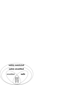
Figure 2: Chase termination conditions.

Figure 2 summarizes the results of this section and puts them into context. First, we will introduce the novel class of safe constraints, which guarantees the termination of the chase. It strictly subsumes weak acyclicity, but is different from stratification. Building upon the definition of safety, we then present safely restricted constraints as a consequent advancement of our ideas. The latter class strictly subsumes all remaining termination conditions known so far. Finally, we will show that, based on our framework, we can easily define another class called safely stratified constraints, which is strictly contained in the class of safely restricted constraints, but also subsumes weak acyclicity and safeness.

Safe Constraints. The basic idea of the first termination condition is to keep track of positions a newly introduced labeled null may be copied to. Consider for instance constraint $R(x_{1},x_{2},x_{3}),S(x_{2})\rightarrow\exists yR(x_{2},y,x_{1})$, which is not weakly acyclic. Its dependency graph is depicted in Figure 3 (left). As illustrated in the toy example in the beginning of this section, a cascading of labeled nulls (i.e. new labeled null values that are created over and over again) may cause a non-terminating chase sequence. However, we can observe that for the constraint above such a cascading of fresh labeled nulls cannot occur, i.e. no fresh labeled null can repeatedly create new labeled nulls in position $R^{2}$ while copying itself to position $R^{1}$. The reason is that the constraint cannot be violated with a fresh labeled null in $R^{2}$, i.e. if $R(a_{1},a_{2},a_{3})$ and $S(a_{2})$ hold, but $\exists yR(a_{2},y,a_{1})$ does not, then $a_{2}$ is never a newly created labeled null. This is due to the fact that $a_{2}$ must also occur in relation $S$, which is not modified when chasing only with this single constraint. Consequently, the chase sequence always terminates. We will later see that this is not a mere coincidence: the constraint is safe.

To formally define safety, we first introduce the notion of affected positions. Intuitively, a position is affected if, during the application of the chase, a newly introduced labeled null can be copied or created in it. Thus, the set of affected positions is an overestimation of the positions in which a null value that was introduced during the chase may occur.

Definition 8

[4] Let $\Sigma$ be a set of TGDs. The set of affected positions $\mbox{aff}(\Sigma)$ of $\Sigma$ is defined inductively as follows. Let $\pi$ be a position in the head of an $\alpha\in$ $\Sigma$.

• If an existentially quantified variable appears in $\pi$, then $\pi\in\mbox{aff}(\Sigma)$.

• If the same universally quantified variable $X$ appears both in position $\pi$, and only in affected positions in the body of $\alpha$, then $\pi\in\mbox{aff}(\Sigma)$. $\Box$

Although we borrow this definition from [4] our focus is different. We extend known classes of constraints for which the chase terminates. The focus in [4] is on query answering in cases the chase may not terminate. Our work neither subsumes [4] nor the other way around. Like in the case of weak acyclicity, we define the safety condition with the help of the absence of cycles containing special edges in some graph. We call this graph propagation graph.

Definition 9

Given a set of TGDs $\Sigma$, the propagation graph $\mbox{prop}(\Sigma):=(\mbox{aff}(\Sigma),E)$ is the directed graph defined as follows. There are two kinds of edges in $E$. Add them as follows: for every TGD $\forall\overline{x}(\phi(\overline{x})\rightarrow\exists\overline{y}\psi(\overline{x},\overline{y}))\in\Sigma$ and for every $x$ in $\overline{x}$ that occurs in $\psi$ and every occurrence of $x$ in $\phi$ in position $\pi_{1}$

• if $x$ occurs only in affected positions in $\phi$ then, for every occurrence of $x$ in $\psi$ in position $\pi_{2}$, add an edge $\pi_{1}\rightarrow\pi_{2}$ (if it does not already exist).

• if $x$ occurs only in affected positions in $\phi$ then, for every existentially quantified variable $y$ and for every occurrence of $y$ in a position $\pi_{2}$, add a special edge $\pi_{1}\stackrel{{\scriptstyle*}}{{\rightarrow}}\pi_{2}$ (if it does not already exist).$\Box$

Figure 3: Left: Dependency graph. Right: Corresponding propagation graph (it has no edges).

Definition 10

A set $\Sigma$ of constraints is called safe iff $\mbox{prop}(\Sigma)$ has no cycles going through a special edge. $\Box$

The intuition of these definitions is that we forbid an unrestricted cascading of null values, i.e. with the help of the propagation graph we impose a partial order on the affected positions such that any newly introduced null value can only be created in a position that has a higher rank in that partial order in comparison to null values that may occur in the body of a TGD. To state this more precisely, assume a TGD of the form $\forall\overline{x}(\phi(\overline{x})\rightarrow\exists\overline{y}\psi(\overline{x},\overline{y}))$ is violated. Then, $I\models\phi(\overline{a})$ and $I\nvDash\exists\overline{y}\psi(\overline{a},\overline{y}))$ must hold. The safety condition ensures that any position in the body that has a newly created labeled null from $\overline{a}$ in itself and also occurs in the head of the TGD has a strictly lower rank in our partial order than any position in which some element from $\overline{y}$ occurs. The main difference in comparison to weak acyclicity is that we look in a refined way (see affected positions) on where a labeled null can be propagated to. We note that given a set of constraints it can be decided in polynomial time whether it is safe.

Example 4

Consider the TGD $R(x_{1},x_{2},x_{3}),S(x_{2})\rightarrow\exists yR(x_{2},y,x_{1})$ from before. The dependency graph is depicted in Figure 3 on the left side and its propagation graph on the right side. The only affected position is $R^{2}$. From the respective definitions it follows that this constraint is safe, but not weakly acyclic. $\Box$

Note that if $\Sigma$ is safe, then every subset of $\Sigma$ is safe, too. We will now compare safety to other termination conditions. In the example, the propagation graph is a subgraph of the dependency graph. This is not a mere coincidence.

Theorem 7

Let $\Sigma$ be a set of constraints.

• Then, $\mbox{prop}(\Sigma)$ is a subgraph of $\mbox{dep}(\Sigma)$. It holds that if $\Sigma$ is weakly acyclic, then it is also safe.

• There is some $\Sigma$ that is safe, but not stratified.

• There is some $\Sigma$ that is stratified, but not safe. $\Box$

The next result shows that safety guarantees termination while retaining polynomial time data complexity.

Theorem 8

Let $\Sigma$ be a fixed set of safe constraints. Then, there exists a polynomial $Q\in\mathbb{N}[X]$ such that for any database instance $I$, the length of every chase sequence is bounded by $Q(||I||)$, where $||I||$ is the number of distinct values in $I$. $\Box$

Safely Restricted Constraints. In this section we generalize the method of stratification from [8] to a condition which we call safe restriction. The chase graph from [8] will be a special case of our new notion. We then define the notion of safe restriction and show that the chase always terminates for constraints obeying it.

Let $\alpha:=S(x_{2},x_{3}),R(x_{1},x_{2},x_{3})\rightarrow\exists yR(x_{2},y,x_{1})$ and $\beta:=R(x_{1},x_{2},x_{3})\rightarrow S(x_{1},x_{3})$. It can be seen that $\alpha\prec\beta$ and $\beta\prec\alpha$. Further, $\{\alpha,\beta\}$ is not weakly acyclic, so it follows that $\{\alpha,\beta\}$ is not stratified. Still, the chase will always terminate: A firing of $\alpha$ may cause a null value to appear in position $R^{2}$, but a firing of $\beta$ will never introduce null values in the head of $\beta$ although $\beta\prec\alpha$ holds. This is the key observation for the upcoming definitions. First, we will refine the relation $\prec$ from [8]. This refinement helps us to detect if during the chase null values might be copied to the head of some constraint. Let $pos(\Sigma)$ denote the set of positions that occur in the body of some constraint in $\Sigma$.

Definition 11

Let $\Sigma$ a set of constraints and $P\subseteq pos(\Sigma)$. For all $\alpha,\beta\in\Sigma$, we define $\alpha\prec_{P}\beta$ iff there are tuples $\overline{a},\overline{b}$ and a database instance $I$ s.t.

• $I\nvDash\alpha(\overline{a})$,

• $\beta$ is not applicable on $\overline{b}$ and $I$,

• $I\overline{a}\oplus C_{\alpha}\nvDash\beta(\overline{b})$,

• null values in $I$ occur only in positions from $P$, and

• the firing of $\beta$ in the case of bullet three copies some null value from $I\overline{a}\oplus C_{\alpha}$ to the head of $\beta$. $\Box$

We next introduce a notion for affected positions relative to a constraint and a set of positions.

Definition 12

For any set of positions $P$ and tgd $\alpha$ let $\mbox{aff-cl}(\alpha,P)$ be the set of positions $\pi$ from the head of $\alpha$ such that either

• the variable in $\pi$ occurs in the body of $\alpha$ only in positions from $P$ or

• $\pi$ contains an existentially quantified variable. $\Box$

The latter definition and the refinement of $\prec$ will help us to define the notion of a restriction system, which is a strict generalization of the chase graph introduced in [8].

Definition 13

A restriction system is a pair $(G^{\prime}(\Sigma),f)$, where $G^{\prime}(\Sigma):=(\Sigma,E)$ is a directed graph and $f:\Sigma\rightarrow 2^{pos(\Sigma)}$ is a function such that

• forall TGDs $\alpha$ and forall $(\alpha,\beta)\in E$:
  $\mbox{aff-cl}(\alpha,f(\alpha))\cap pos(\{\beta\})\subseteq f(\beta)$,

• forall EGDs $\alpha$ and forall $(\alpha,\beta)\in E$:
  $f(\alpha)\cap pos(\{\beta\})\subseteq f(\beta)$, and

• forall $\alpha,\beta\in\Sigma$: $\alpha\prec_{f(\alpha)}\beta\implies(\alpha,\beta)\in E$.$\Box$

We illustrate this definition by an example. It also shows that restriction systems always exist.

Example 5

Let $\Sigma$ a set of constraints. Then, $(G(\Sigma),f)$, where $f(\alpha):=pos(\{\alpha\})$ for all $\alpha\in\Sigma$ is a restriction system for $\Sigma$. $\Box$

Based on the novel technical notion of restriction systems we can easily define a new class of constraints.

Definition 14

$\Sigma$ is called safely restricted if and only if there is a restriction system $(G^{\prime}(\Sigma),f)$ for $\Sigma$ such that every strongly connected component in $G^{\prime}(\Sigma)$ is safe. $\Box$

The next theorem shows that safe restriction strictly extends the notion of stratification and safety.

Theorem 9

If $\Sigma$ is stratified or safe, then it is also safely restricted. There is some $\Sigma$ that is safely restricted but neither safe nor stratified. $\Box$

Definition 14 implies that safely restricted constraints can be recognized by a $\Sigma_{2}^{P}$-algorithm. However, with the help of a canonical restriction system, we can show that safe restriction can be decided in coNP (like stratification).

Theorem 10

Given constraint set $\Sigma$ it can be checked by a coNP-algorithm whether $\Sigma$ is safely restricted. $\Box$

The next theorem is the main contribution of this section. It states that the chase will always terminate in polynomial time data complexity for safely restricted constraints.

Theorem 11

Let $\Sigma$ be a fixed set of safely restricted constraints. Then, there exists a polynomial $Q\in\mathbb{N}[X]$ such that for any database instance $I$, the length of every chase sequence is bounded by $Q(||I||)$, where $||I||$ is the number of distinct values in $I$. $\Box$

To the best of our knowledge safe restriction is the most general sufficient termination condition for TGDs and EGDs. We finally compare the chase graph to restriction systems. The reader might wonder what happens if we substitute weak acyclicity with safety in the definition of stratification (in the preliminaries).

Definition 15

We call $\Sigma$ safely stratified iff the constraints in every cycle of $G(\Sigma)$ are safe. $\Box$

We obtain the following result, showing that with the help of restriction systems, we strictly extended the method of the chase graph from [8].

Theorem 12

Let $\Sigma$ be a set of constraints.

• If $\Sigma$ is weakly acyclic or safe, then it is safely stratified.

• If $\Sigma$ is safely stratified, then it is safely restricted.

• There is some set of constraints that is safely restricted, but not safely stratified. $\Box$

Note that we used safety instead of safe stratification in the definition of safe restrictedness although safely stratified constraints are the provably larger class. This is due to the fact that safety is easily checkable and would not change the class of constraints. The next proposition clarifies this issue.

Proposition 3

$\Sigma$ is safely restricted iff there is a restriction system $(G^{\prime}(\Sigma),f)$ for $\Sigma$ such that every strongly connected component in $G^{\prime}(\Sigma)$ is safely stratified. $\Box$

In the previous section we proposed two SPARQL translation schemes and it is left to explain why we introduced two alternative schemes. The next proposition states that the two schemes behave differently with respect to safe restriction.

Proposition 4

Let $\Sigma$ be a non-empty set of constraint set over a ternary relation symbol $T$.

• There is some $\Sigma$ that is safely restricted, but $\Sigma^{\prime}=\emptyset$, i.e. the second translation scheme is not applicable.

• There is some $\Sigma$ such that $|\Sigma|=|\Sigma^{\prime}|$ and $\Sigma^{\prime}$ is safely restricted, but $\Sigma$ is not. $\Box$

Referring back to Lemma 3, this means we might check both $\Sigma$ or $\Sigma^{\prime}$ for safe restrictedness, and can guarantee termination of the chase if at least one of them is safely restricted.

7 Conclusion

We have discussed several facets of the SPARQL query language. Our complexity analysis extends prior investigations [26] and (a) shows that the combination of And and Union is the main source of complexity in Opt-free SPARQL fragments and (b) clarifies that yet operator Opt alone makes SPARQL evaluation PSpace-complete. We also show that, when restricting the nesting depth of Opt-expressions, we obtain better complexity bounds.

The subsequent study of SPARQL Algebra lays the foundations for transferring established Relational Algebra optimization techniques into the context of SPARQL. Additionally, we considered specifics of the SPARQL query language, such as rewriting of SPARQL queries involving negation. The algebraic optimization approach is complemented by a powerful framework for semantic query optimization. We argue that a combination of both algebraic and semantic optimization will push the limits of existing SPARQL implementations and leave the study of a schematic rewriting approach and good rewriting heuristics as future work.

Finally, our results on chase termination empower the practicability of SPARQL query optimization in the presence of constraints and directly carry over to other applications that rely on the chase, such as [28, 20, 15, 9].

Appendix A Proofs of the Complexity Results

This section contains the complexity proofs of the Evaluation problem for the fragments studied in Section 3. We refer the interested reader to [26] for the proof of Theorem 1. We start with some basics from complexity theory.

A.1 Background from Complexity Theory

Complexity Classes. As usual, we denote by PTime (or P, for short) the complexity class comprising all problems that can be decided by a deterministic Turing Machine (TM) in polynomial time, by NP the set of problems that can be decided by a non-deterministic TM in polynomial time, and by PSpace the class of problems that can be decided by a deterministic TM within polynomial space bounds.

The Polynomial Hierarchy

Given a complexity class C we denote by coC the set of decision problems whose complement can be decided by a TM in class C. Given complexity classes $\textsc{C}_{1}$ and $\textsc{C}_{2}$, the class $\textsc{C}_{1}^{\textsc{C}_{2}}$ captures all problems that can be decided by a TM $M_{1}$ in class $\textsc{C}_{1}$ enhanced by an oracle TM $M_{2}$ for solving problems in class $\textsc{C}_{2}$. Informally, engine $M_{1}$ can use $M_{2}$ to obtain a yes/no-answer for a problem in $\textsc{C}_{2}$ in a single step. We refer the interested reader to [2] for a more formal discussion of oracle machines. Finally, we define the classes $\Sigma^{P}_{i}$ and $\Pi^{P}_{i}$ recursively as

$\Sigma^{P}_{0}=\Pi^{P}_{0}{:=}\textsc{P}$ and $\Sigma^{P}_{n+1}{:=}\textsc{NP}^{\Sigma^{P}_{n}}$, and put

$\Pi^{P}_{n+1}{:=}\textsc{coNP}^{\Sigma^{P}_{n}}$.

The polynomial hierarchy PH [30] is then defined as

$\textsc{PH}=\bigcup_{i\in\mathbb{N}_{0}}\Sigma^{P}_{i}$

It is folklore that $\Sigma^{P}_{i}=co\Pi^{P}_{i}$, and that $\Sigma^{P}_{i}\subseteq\Pi^{P}_{i+1}$ and $\Pi^{P}_{i}\subseteq\Sigma^{P}_{i+1}$ holds. Moreover, the following inclusion hierarchies for $\Sigma^{P}_{i}$ and $\Pi^{P}_{i}$ are known.

$\textsc{P}=\Sigma^{P}_{0}\subseteq\textsc{NP}=\Sigma^{P}_{1}\subseteq\Sigma^{P}_{2}\subseteq\dots\subseteq\textsc{PSPACE}$, and

$\textsc{P}=\Pi^{P}_{0}\subseteq\textsc{coNP}=\Pi^{P}_{1}\subseteq\Pi^{P}_{2}\subseteq\dots\subseteq\textsc{PSPACE}$.

Complete Problems

We consider completeness only with respect to polynomial-time many-one reductions. QBF, the tautology test for quantified boolean formulas, is known to be PSpace-complete [2]. Forms of QBF with restricted quantifier alternation are complete for classes $\Pi^{P}_{i}$ or $\Sigma^{P}_{i}$ depending on the question if the first quantified of the formula is $\forall$ or $\exists$. A more thorough introduction to complete problems in the polynomial hierarchy can be found in [2]. Finally, the NP-completeness of the SetCover-problem and the 3Sat-problem is folklore.

A.2 OPT-free Fragments (Theorem 2)

Fragment $\cal{U}$: UNION (Theorem 2(1))

For a Union-only expression $P$ and data set $D$ it suffices to check if $\mu\in{\llbracket t\rrbracket_{D}}$ for any triple pattern $t$ in $P$. This can easily be achieved in polynomial time.$\hskip 1.0pt\Box$

Fragment $\cal{FU}$: FILTER + UNION (Theorem 2(1))

We present a PTime-algorithm that solves the Evaluation problem for this fragment. It is defined on the structure of the input expression $P$ and returns true if $\mu\in{\llbracket P\rrbracket_{D}}$, false otherwise. We distinguish three cases. (a) If $P=t$ is a triple pattern, we return true if and only if $\mu\in{\llbracket t\rrbracket_{D}}$. (b) If $P=P_{1}{\ \textsc{Union}\ }P_{2}$ we (recursively) check if $\mu\in{\llbracket P_{1}\rrbracket_{D}}\lor\mu\in{\llbracket P_{2}\rrbracket_{D}}$ holds. (c) If $P=P_{1}{\ \textsc{Filter}\ }R$ for any filter condition $R$ we return true if and only if $\mu\in{\llbracket P_{1}\rrbracket_{D}}\land R\models\mu$. It is easy to see that the above algorithm runs in polynomial time. Its correctness follows from the definition of the algebraic operators $\cup$ and ${\sigma}$.$\hskip 1.0pt\Box$

Fragment $\cal{AU}$: AND + UNION (Theorem 2(2))

In order to show that Evaluation for this fragment is NP-complete we have to show membership and hardness.

Membership in NP. Let $P$ be a SPARQL expression composed of operators And and Union, $D$ a document, and $\mu$ a mapping. We provide an NP-algorithm that returns true if $\mu\in{\llbracket P\rrbracket_{D}}$, and false otherwise. Our algorithm is defined on the structure of $P$. (a) If $P=t$ return true if $\mu\in{\llbracket t\rrbracket_{D}}$, false otherwise. (b) If $P=P_{1}{\ \textsc{Union}\ }P_{2}$, we return the truth value of $\mu\in{\llbracket P_{1}\rrbracket_{D}}\lor\mu\in{\llbracket P_{2}\rrbracket_{D}}$. (c) If $P=P_{1}{\ \textsc{And}\ }P_{2}$, we guess a decomposition $\mu=\mu_{1}\cup\mu_{2}$ and return the truth value of $\mu_{1}\in{\llbracket P_{1}\rrbracket_{D}}\land\mu_{2}\in{\llbracket P_{2}\rrbracket_{D}}$. Correctness of the algorithm follows from the definition of the algebraic operators $\Join$ and $\cup$. It can easily be realized by a non-deterministic TM that runs in polynomial time, which proves membership in NP.

NP-Hardness. We reduce the SetCover problem to the Evaluation problem for SPARQL (in polynomial time). SetCover is known to be NP-complete, so the reduction gives us the desired hardness result.

The decision version of SetCover is defined as follows. Let $U=\{u_{1},\dots,u_{k}\}$ be a universe, $S_{1},\dots S_{n}\subseteq U$ be sets over $U$, and let $k$ be positive integer. Is there a set $I\subseteq\{1,\dots,n\}$ of size $\mid I\mid\leq k$ s.t. $\bigcup_{i\in I}S_{i}=U$?

We use the fixed database $D:=\{(a,b,1)\}$ for our encoding and represent each set $S_{i}=\{x_{1},x_{2},\dots,x_{m}\}$ by a SPARQL expression of the form

$P_{S_{i}}:=(a,b,?X_{1}){\ \textsc{And}\ }\dots\ \textsc{And}\ (a,b,?X_{m})$.

The set $S=\{S_{1},\dots,S_{n}\}$ of all $S_{i}$ is then encoded as

$P_{S}:=P_{S_{1}}{\ \textsc{Union}\ }\dots\ \textsc{Union}\ P_{S_{n}}$.

Finally we define the SPARQL expression

$P:=P_{S}{\ \textsc{And}\ }\dots\ \textsc{And}\ P_{S}$,
	where $P_{S}$ appears exactly $k$ times.

It is straightforward to show that SetCover is true if and only if $\mu=\{?U_{1}\mapsto 1,\dots,?U_{k}\mapsto 1\}\in{\llbracket P\rrbracket_{D}}$. The intuition of the encoding is as follows. $P_{S}$ encodes all subsets $S_{i}$. A set element, say $x$, is represented in SPARQL by a mapping from variable $?X$ to value $1$. The encoding of $P$ allows us to merge (at most) $k$ arbitrary sets $S_{i}$. We finally check if the universe $U$ can be constructed this way.$\hskip 1.0pt\Box$

Remark 2

The proof above relies on the fact that mapping $\mu$ is part of the input of the Evaluation problem. In fact, when fixing $\mu$ the resulting (modified) version of the Evaluation problem can be solved in PTime.$\Box$

A.3 Fragments Including Operator OPT

We now discuss several fragments including Opt. One goal here is to show that fragment $\cal{O}$ is PSpace-complete (c.f. Theorem 3); PSpace-completeness for all fragments involving Opt then follows (cf. Corollary 1). Given the PSpace-completeness results for fragment $\cal{E}=\cal{AFOU}$, it suffices to prove hardness for all smaller fragments; membership is implicit. Our road map is as follows.

1. We first show PSpace-hardness for fragment $\cal{AFO}$.

2. We then show PSpace-hardness for fragment $\cal{AO}$.

3. Next, a rewriting of operator And by Opt is presented, which can be used to eliminate all And operators in the proof of (2). PSpace-completeness for $\cal{O}$ then is shown using this rewriting rule.

4. Finally, we prove Theorem 4, i.e. show that fragment $\cal{E}$_≤n is $\Sigma^{P}_{n+1}$-complete, making use of part (1).

Fragment $\cal{AFO}$: AND + FILTER + OPT

We present a (polynomial-time) reduction from QBF to Evaluation for fragment $\cal{AFO}$. The QBF problem is known to be PSpace-complete, so this reduction gives us the desired PSpace-hardness result. Membership in PSpace, and hence PSpace-completeness, then follows from Theorem 1(3). QBF is defined as follows.

	QBF: given a quantified boolean formula of the form
			$\varphi=\forall x_{1}\exists y_{1}\forall x_{2}\exists y_{2}\dots\forall x_{m}\exists y_{m}\psi$,
		where $\psi$ is a quantifier-free boolean formula,
		as input: is $\varphi$ valid?

The following proof was inspired by the proof of Theorem 3 in [26]: we encode the inner formula $\psi$ using And and Filter, and then adopt the translation scheme for the quantifier sequence $\forall\exists\forall\exists\dots$ proposed in [26].

First note that, according to the problem statement, $\psi$ is a quantifier-free boolean formula. We assume w.l.o.g. that $\psi$ is composed of $\land$, $\lor$ and $\neg$. We use the fixed database

$D:=\{(a,\textit{tv},0),(a,\textit{tv},1),(a,\textit{false},0),(a,\textit{true},1)\}$

and denote by $V=\{v_{1},\dots v_{l}\}$ the set of variables appearing in $\psi$. Formula $\psi$ then is encoded as

$P_{\psi}{:=}((a,tv,?V_{1}){\ \textsc{And}\ }(a,tv,?V_{2}){\ \textsc{And}\ }\dots$
	${\ \textsc{And}\ }(a,tv,?V_{l})){\ \textsc{Filter}\ }{\it f}(\psi)$,

where ${\it f}(\psi)$ is a function that generates a SPARQL condition that mirrors the boolean formula $\psi$. More precisely, ${\it f}$ is defined recursively on the structure of $\psi$ as

f($v_{i}$)	${:=}$	$?V_{i}$ = 1
f($\psi_{1}\land\psi_{2}$)	${:=}$	f($\psi_{1}$) $\land$ f($\psi_{2}$)
f($\psi_{1}\lor\psi_{2}$)	${:=}$	f($\psi_{1}$) $\lor$ f($\psi_{2}$)
f($\neg\psi_{1}$)	${:=}$	$\neg$ f($\psi_{1}$)

In our encoding $P_{\psi}$, the And-block generates all possible valuations for the variables, while the Filter-expression retains exactly those valuations that satisfy formula $\psi$. It is straightforward to show that $\psi$ is satisfiable if and only if there exists a mapping $\mu\in{\llbracket P_{\psi}\rrbracket_{D}}$ and, moreover, for each mapping $\mu\in{\llbracket P_{\psi}\rrbracket_{D}}$ there is a truth assignment $\rho_{\mu}$ defined as $\rho_{\mu}(x)=\mu(?X)$ for all variables $?X_{i},?Y_{i}\in{\it dom}(\mu)$ such that $\mu\in{\llbracket P_{\psi}\rrbracket_{D}}$ if and only if $\rho_{\mu}$ satisfies $\psi$. Given $P_{\psi}$, we can encode the quantifier-sequence using a series of nested Opt statements as shown in [26]. To make the proof self-contained, we shortly summarize this construction.

SPARQL variables $?X_{1},\dots,?X_{m}$ and $?Y_{1},\dots Y_{m}$ are used to represent variables $x_{1},\dots x_{m}$ and $y_{1},\dots,y_{m}$, respectively. In addition to these variables, we use fresh variables $?A_{0},\dots?A_{m}$, $?B_{0},\dots?B_{m}$, and operators And and Opt to encode the quantifier sequence $\forall x_{1}\exists y_{1}\dots\forall x_{m}\exists y_{m}$. For each $i\in[m]$ we define two expressions $P_{i}$ and $Q_{i}$

$P_{i}$	${:=}$	$((a,tv,?X_{1}){\ \textsc{And}\ }\dots\ \textsc{And}\ (a,tv,?X_{i}){\ \textsc{And}\ }$
		$\ \ (a,tv,?Y_{1}){\ \textsc{And}\ }\dots\ \textsc{And}\ (a,tv,?Y_{i-1}){\ \textsc{And}\ }$
		$\ \ (a,{\it false},?A_{i-1}){\ \textsc{And}\ }(a,{\it true},?A_{i}))$,
$Q_{i}$	${:=}$	$((a,tv,?X_{1}){\ \textsc{And}\ }\dots\ \textsc{And}\ (a,tv,?X_{i}){\ \textsc{And}\ }$
		$\ \ (a,tv,?Y_{1}){\ \textsc{And}\ }\dots\ \textsc{And}\ (a,tv,?Y_{i}){\ \textsc{And}\ }$
		$\ \ (a,{\it false},?B_{i-1}){\ \textsc{And}\ }(a,{\it true},?B_{i}))$,

and encode $P_{\varphi}$ as

$P_{\varphi}{:=}$	$((a,{\it true},?B_{0})$
		${\ \textsc{Opt}\ }(P_{1}{\ \textsc{Opt}\ }(Q_{1}$
			${\ \textsc{Opt}\ }(P_{2}{\ \textsc{Opt}\ }(Q_{2}$
				$\dots$
				${\ \textsc{Opt}\ }(P_{m}{\ \textsc{Opt}\ }(Q_{m}{\ \textsc{And}\ }P_{\psi}))\dots)))))$

It can be shown that $\mu=\{?B_{0}\mapsto 1\}\in{\llbracket P_{\varphi}\rrbracket_{D}}$ iff $\varphi$ is valid, which completes the reduction. We refer the reader to the proof of Theorem 3 in [26] for this part of the proof.$\hskip 1.0pt\Box$

Remark 3

The proof for this fragment ($\cal{AFO}$) is subsumed by the subsequent proof, which shows PSpace-hardness for a smaller fragment. It was included to illustrate how to encode quantifier-free boolean formulas that are not in CNF. Some of the following proofs build upon this construction.$\Box$

Fragment $\cal{AO}$: AND + OPT

We reduce the QBF problem to Evaluation for class $\cal{AO}$. We encode a quantified boolean formula of the form

$\varphi=\forall x_{1}\exists y_{1}\forall x_{2}\exists y_{2}\dots\forall x_{m}\exists y_{m}\psi$,

where $\psi$ is a quantifier-free formula in conjunctive normal form (CNF), i.e. $\psi$ is a conjunction of clauses

$\psi=C_{1}\land\dots\land C_{n}$,

where the $C_{i}$, $1\leq i\leq n$, are disjunctions of literals. By $V$ we denote the variables in $\psi$ and by $V_{C_{i}}$ the variables appearing in clause $C_{i}$ (either as positive of negative literals). We use the following database, which is polynomial in the size of the query.

$D:=$	$\{(a,\textit{tv},0),(a,\textit{tv},1),(a,\textit{false},0),(a,\textit{true},1)\}\ \cup$
	$\{(a,var_{i},v)\mid v\in V_{C_{i}}\}\ \cup\ \{(a,v,v)\mid v\in V\}$

For each $C_{i}=v_{1}\lor\dots\lor v_{j}\lor\neg v_{j+1}\lor\dots\lor\neg v_{k}$, where the $v_{1}\dots v_{j}$ are positive and the $v_{j+1}\dots v_{k}$ are negated variables (contained in $V_{C_{i}}$), we define a separate SPARQL expression

$P_{C_{i}}{:=}(\dots((\dots($
	$(a,var_{i},?var_{i})$
		$\ \textsc{Opt}\ ((a,v_{1},?var_{i}){\ \textsc{And}\ }(a,true,?V_{1})))$
			$\ \ \ldots$
				$\ \ \ \textsc{Opt}\ ((a,v_{j},?var_{i}){\ \textsc{And}\ }(a,true,?V_{j})))$
					$\ \ \ \ \textsc{Opt}\ ((a,v_{j+1},?var_{i}){\ \textsc{And}\ }(a,false,?V_{j+1})))$
						$\ \ \ \ \ \ldots$
							$\ \ \ \ \ \ \textsc{Opt}\ ((a,v_{k},?var_{i}){\ \textsc{And}\ }(a,false,?V_{k})))$

and encode formula $\psi$ as

$P_{\psi}:=P_{C_{1}}{\ \textsc{And}\ }\dots\ \textsc{And}\ P_{C_{n}}$.

It is straightforward to verify that $\psi$ is satisfiable if and only if there is a mapping $\mu\in{\llbracket P_{\psi}\rrbracket_{D}}$ and, moreover, for each $\mu\in{\llbracket P_{\psi}\rrbracket_{D}}$ there is a truth assignment $\rho_{\mu}$ defined as $\rho_{\mu}(x)=\mu(?X)$ for all variables $?X_{i},?Y_{i}\in{\it dom}(\mu)$ such that $\mu\in{\llbracket P_{\psi}\rrbracket_{D}}$ if and only if $\rho_{\mu}$ satisfies $\psi$. Now, given $P_{\psi}$, we encode the quantifier-sequence using only operators Opt and And, as shown in the previous proof for fragment $\cal{AFO}$. For the resulting encoding $P_{\varphi}$, it analogously holds that $\mu=\{?B_{0}\mapsto 1\}\in{\llbracket P_{\varphi}\rrbracket_{D}}$ iff $\varphi$ is valid.$\hskip 1.0pt\Box$

We provide a small example that illustrates the translation scheme for QBF presented in in the proof above.

Example 6

We show how to encode the QBF

$\varphi$	$=\forall x_{1}\exists y_{1}(x_{1}\Leftrightarrow y_{1})$
	$=\forall x_{1}\exists y_{1}((x_{1}\lor\neg y_{1})\land(\neg x_{1}\lor y_{1}))$,

where $\psi=((x_{1}\lor\neg y_{1})\land(\neg x_{1}\lor y_{1}))$ is in CNF. It is easy to see that the QBF formula $\varphi$ is a tautology. The variables in $\psi$ are $V=\{x_{1},y_{1}\}$; further, we have $C_{1}=x_{1}\lor\neg y_{1}$, $C_{2}=\neg x_{1}\lor y_{1}$, and $V_{C_{1}}=V_{C_{2}}=V=\{x_{1},y_{1}\}$. Following the construction in the proof we set up the database

$D:=\${	$(a,\textit{tv},0),(a,\textit{tv},1),(a,\textit{false},0),(a,\textit{true},1),$
	$(a,var_{1},x_{1}),(a,var_{1},y_{1}),(a,var_{2},x_{1}),$
	$(a,var_{2},y_{1}),(a,x_{1},x_{1}),(a,y_{1},y_{1})\}$

and define expression $P_{\psi}=P_{C_{1}}{\ \textsc{And}\ }P_{C_{2}}$, where

$P_{C_{1}}{:=}((a,var_{1},?var_{1})$
	${\ \textsc{Opt}\ }((a,x_{1},?var_{1}){\ \textsc{And}\ }(a,true,?X_{1})))$
		${\ \textsc{Opt}\ }((a,y_{1},?var_{1}){\ \textsc{And}\ }(a,false,?Y_{1}))$
$P_{C_{2}}{:=}((a,var_{2},?var_{2})$
	${\ \textsc{Opt}\ }((a,y_{1},?var_{2}){\ \textsc{And}\ }(a,true,?Y_{1})))$
		${\ \textsc{Opt}\ }((a,x_{1},?var_{2}){\ \textsc{And}\ }(a,false,?X_{1}))$.

When evaluating these expressions we get:

	${\llbracket P_{C_{1}}\rrbracket_{D}}$	$=(\{\{?var_{1}\mapsto x_{1}\},\{?var_{1}\mapsto y_{1}\}\}$
			${\ \louterjoin\ }\{\{?var_{1}\mapsto x_{1},?X_{1}\mapsto 1\}\})$
				${\ \louterjoin\ }\{\{?var_{1}\mapsto y_{1},?Y_{1}\mapsto 0\}\}$
	$=\{\{?var_{1}\mapsto x_{1},?X_{1}\mapsto 1\},\{?var_{1}\mapsto y_{1},?Y_{1}\mapsto 0\}\}$
	${\llbracket P_{C_{2}}\rrbracket_{D}}$	$=\{\{?var_{2}\mapsto x_{1}\},\{?var_{2}\mapsto y_{1}\}\}$
			${\ \louterjoin\ }\{\{?var_{2}\mapsto y_{1},?Y_{1}\mapsto 1\}\}$
				${\ \louterjoin\ }\{\{?var_{2}\mapsto x_{1},?X_{1}\mapsto 0\}\}$
	$=\{\{?var_{2}\mapsto x_{1},?X_{1}\mapsto 0\},\{?var_{2}\mapsto y_{2},?Y_{2}\mapsto 1\}\}$
	${\llbracket P_{\psi}\rrbracket_{D}}$	$={\llbracket P_{C_{1}}{\ \textsc{And}\ }P_{C_{2}}\rrbracket_{D}}$
	$=\{\{?var_{1}\mapsto x_{1},?var_{2}\mapsto y_{1},?X_{1}\mapsto 1,?Y_{1}\mapsto 1\},$
	$\ \ \ \ \ \ \ \{?var_{1}\mapsto y_{1},?var_{2}\mapsto x_{1},?X_{1}\mapsto 0,?Y_{1}\mapsto 0\}\}$

Finally, we set up the expressions $P_{1}$ and $Q_{1}$, as described in the proof for fragment $\cal{AOF}$

$P_{1}$	${:=}$	$((a,tv,?X_{1}){\ \textsc{And}\ }(a,{\it false},?A_{0})$
		${\ \textsc{And}\ }(a,{\it true},?A_{1}))$
$Q_{1}$	${:=}$	$((a,tv,?X_{1}){\ \textsc{And}\ }(a,tv,?Y_{1})$
		${\ \textsc{And}\ }(a,{\it false},?B_{0}){\ \textsc{And}\ }(a,{\it true},?B_{1}))$

and encode the quantified boolean formula $\varphi$ as

$P_{\varphi}:=(a,{\it true},?B_{0}){\ \textsc{Opt}\ }(P_{1}{\ \textsc{Opt}\ }(Q_{1}{\ \textsc{And}\ }P_{\psi}))$

We leave it as an exercise to verify that the mapping $\mu=\{?B_{0}\mapsto 1\}$ is contained in ${\llbracket P_{\varphi}\rrbracket_{D}}$. This result confirms that the original formula $\psi$ is valid.$\Box$

Fragment $\cal{O}$: OPT-only (Theorem 3)

We start with a transformation rule for operator And; it essentially expresses the key idea of the subsequent proof.

Lemma 7

Let

• $Q,Q_{1},Q_{2},\dots,Q_{n}$ ($n\geq 2$) be SPARQL expressions,

• $S=\it{vars}(Q)\cup\it{vars}(Q_{1})\cup{\it vars}(Q_{2})\cup\dots\cup\it{vars}(Q_{n})$, denote the set of variables in $Q,Q_{1},Q_{2},\dots,Q_{n}$

• $D=\{(a,true,1),(a,false,0),(a,tv,0),(a,tv,1)\}$ be a fixed database,

• $?V_{2},?V_{3},\dots,?V_{n}$ be a set of $n-1$ fresh variables, i.e. $S\cap\{?V_{2},?V_{3},\dots,?V_{n}\}=\emptyset$ holds.

Further, we define

$Q^{\prime}{:=}((\dots((Q{\ \textsc{Opt}\ }V_{2}){\ \textsc{Opt}\ }V_{3})\dots){\ \textsc{Opt}\ }V_{n})$,
$Q^{\prime\prime}{:=}((\dots((Q_{1}{\ \textsc{Opt}\ }(Q_{2}{\ \textsc{Opt}\ }V_{2}))$
	${\ \textsc{Opt}\ }(Q_{3}{\ \textsc{Opt}\ }V_{3}))$
		$\dots$
		${\ \textsc{Opt}\ }(Q_{n}{\ \textsc{Opt}\ }V_{n}))),$
$V_{i}{:=}(a,true,?V_{i})$, and
$\overline{V}_{i}{:=}(a,false,?V_{i})$.

The following claims hold.

(1) ${\llbracket Q^{\prime}\rrbracket_{D}}=\{\mu\cup\{?V_{2}\mapsto 1,\dots,?V_{n}\mapsto 1\}\mid\mu\in{\llbracket Q\rrbracket_{D}}\}$,
(2) ${\llbracket Q^{\prime}{\ \textsc{Opt}\ }(Q_{1}{\ \textsc{And}\ }Q_{2}{\ \textsc{And}\ }\dots\ \textsc{And}\ Q_{n})\rrbracket_{D}}$
	$=\llbracket Q^{\prime}{\ \textsc{Opt}\ }(\dots((Q^{\prime\prime}{\ \textsc{Opt}\ }\overline{V}_{2})$
		${\ \textsc{Opt}\ }\overline{V}_{3})$
		$\ \ \dots$
		${\ \textsc{Opt}\ }\overline{V}_{n})\rrbracket_{D}$

$\Box$

The second part of the lemma provides a way to rewrite an And-only expression that is encapsulated in the right side of an Opt-expression by means of an Opt-only expression. Before proving the lemma, we illustrate the construction by means of a small example.

Example 7

Let $D$ be the database given in the previous lemma and consider the expressions

$Q$	$:=(a,tv,?a)$	,i.e. ${\llbracket Q\rrbracket_{D}}$	$=\{\{?a\mapsto 0\},\{?a\mapsto 1\}\}$
$Q_{1}$	$:=(a,true,?a)$	,i.e. ${\llbracket Q_{1}\rrbracket_{D}}$	$=\{\{?a\mapsto 1\}\}$
$Q_{2}$	$:=(a,false,?b)$	,i.e. ${\llbracket Q_{2}\rrbracket_{D}}$	$=\{\{?b\mapsto 0\}\}$

As for the part (1) of the lemma we observe that

${\llbracket Q^{\prime}\rrbracket_{D}}$	$={\llbracket Q{\ \textsc{Opt}\ }V_{2}\rrbracket_{D}}$
	$={\llbracket Q{\ \textsc{Opt}\ }(a,true,?V_{2})\rrbracket_{D}}$
	$=\{\{?a\mapsto 0,?V_{2}\mapsto 1\},\{?a\mapsto 1,?V_{2}\mapsto 1\}\}$.

Concerning part (2) it holds that the left side

${\llbracket Q^{\prime}{\ \textsc{Opt}\ }(Q_{1}{\ \textsc{And}\ }Q_{2})\rrbracket_{D}}$

$={\llbracket Q^{\prime}\rrbracket_{D}}{\ \louterjoin\ }\{\{?a\mapsto 1,?b\mapsto 0\}\}$

$=\{\{?a\mapsto 0,?V_{2}\mapsto 1\},\{?a\mapsto 1,?b\mapsto 0,?V_{2}\mapsto 1\}\}$

is equal to the right side

${\llbracket Q^{\prime}{\ \textsc{Opt}\ }((Q_{1}{\ \textsc{Opt}\ }(Q_{2}{\ \textsc{Opt}\ }V_{2})){\ \textsc{Opt}\ }\overline{V_{2}})\rrbracket_{D}}$

$={\llbracket Q^{\prime}\rrbracket_{D}}{\ \louterjoin\ }(\{\{?a\mapsto 1,?b\mapsto 0,?V_{2}\mapsto 1\}\}{\ \louterjoin\ }{\llbracket\overline{V_{2}}\rrbracket_{D}})$

$={\llbracket Q^{\prime}\rrbracket_{D}}{\ \louterjoin\ }\{\{?a\mapsto 1,?b\mapsto 0,?V_{2}\mapsto 1\}\}$

$=\{\{?a\mapsto 0,?V_{2}\mapsto 1\},\{?a\mapsto 1,?b\mapsto 0,?V_{2}\mapsto 1\}\}$.$\Box$

Proof of Lemma 7. We omit some technical details, but instead give the intuition of the encoding. (1) The first claim follows trivially from the definition of $Q^{\prime}$, the observations that each $V_{i}$ evaluates to $\{\{?V_{i}\mapsto 1\}\}$, and the fact that all $?V_{i}$ are unbound in $Q^{\prime}$ (recall that, by assumption, the $?V_{i}$ are fresh variables). To prove (2), we consider the evaluation of the right side expression, in order to show that it yields the same result as the left side. First consider subexpression $Q^{\prime\prime}$ and observe that the result of evaluating $Q_{i}{\ \textsc{Opt}\ }V_{i}$ is exactly the result of evaluating $Q_{i}$ extended by the binding $?V_{i}\mapsto 1$. In the sequel, we use $Q^{V}_{i}$ as an abbreviation for $Q_{i}{\ \textsc{Opt}\ }V_{i}$, i.e. we denote $Q^{\prime\prime}$ as $((\dots((Q_{1}{\ \textsc{Opt}\ }Q^{V}_{2}){\ \textsc{Opt}\ }Q^{V}_{3}){\ \textsc{Opt}\ }\dots){\ \textsc{Opt}\ }Q^{V}_{n})$. Applying semantics, we can rewrite ${\llbracket Q^{\prime\prime}\rrbracket_{D}}$ into the form

${\llbracket Q^{\prime\prime}\rrbracket_{D}}$
$=$	${\llbracket((\dots((Q_{1}{\ \textsc{Opt}\ }Q^{V}_{2}){\ \textsc{Opt}\ }Q^{V}_{3}){\ \textsc{Opt}\ }\dots){\ \textsc{Opt}\ }Q^{V}_{n})\rrbracket_{D}}$
$=$	${\llbracket(Q_{1}{\ \textsc{And}\ }Q^{V}_{2}{\ \textsc{And}\ }Q^{V}_{3}{\ \textsc{And}\ }\dots\ \textsc{And}\ Q^{V}_{n})\rrbracket_{D}}\cup P_{D}$,

where we call the left subexpression of the union join part, and $P_{D}$ at the right side is an algebra expression (over database $D$) with the following property: for each mapping $\mu\in P_{D}$ there is at least one $?V_{i}$ ($2\leq i\leq n$) s.t. $?V_{i}\not\in{\it dom}(\mu)$. We observe that, in contrast, for each mapping in the join part ${\it dom}(\mu)\supseteq\{?V_{2},\dots,?V_{n}\}$ holds and, even more, $\mu(?V_{i})=1$, for $2\leq i\leq n$. Hence, the mappings in the result of the join part are identified by the property that $?V_{2},?V_{3},\dots,?V_{n}$ are all bound to 1.

Let us next consider the evaluation of the larger expression (on the right side of the original equation)

$R:=((\dots((Q^{\prime\prime}{\ \textsc{Opt}\ }\overline{V}_{2}){\ \textsc{Opt}\ }\overline{V}_{3}){\ \textsc{Opt}\ }\dots){\ \textsc{Opt}\ }\overline{V}_{n}))$.

When evaluating $R$, we obtain exactly the mappings from ${\llbracket Q^{\prime\prime}\rrbracket_{D}}$, but each mapping $\mu\in{\llbracket Q^{\prime\prime}\rrbracket_{D}}$ is extended by bindings $?V_{i}\mapsto 0$ for all $?V_{i}\not\in{\it dom}(\mu)$ (cf. the argumentation in for claim (1)). As argued before, all mappings in the join part of $Q^{\prime\prime}$ are complete in the sense that all $?V_{i}$ are bound, so these mappings will not be affected. The remaining mappings (i.e. those originating from $P_{D}$) will be extended by bindings $?V_{i}\mapsto 0$ for at least one $?V_{i}$. The resulting situation can be summarized as follows: all mappings resulting from the join part of $Q^{\prime\prime}$ bind all variables $?V_{i}$ to 1; all mappings in $P_{D}$ bind all $?V_{i}$, but at least one of them is bound to 0.

From part (1) we know that each mapping in ${\llbracket Q^{\prime}\rrbracket_{D}}$ maps all $?V_{i}$ to 1. Hence, when computing ${\llbracket Q^{\prime}{\ \textsc{Opt}\ }R\rrbracket_{D}}={\llbracket Q^{\prime}\rrbracket_{D}}{\ \louterjoin\ }{\llbracket R\rrbracket_{D}}$, the bindings $?V_{i}\mapsto 1$ for all $\mu\in{\llbracket Q^{\prime}\rrbracket_{D}}$ serves as a filter that removes the mappings in ${\llbracket R\rrbracket_{D}}$ originating from $P_{D}$. This means

${\llbracket Q^{\prime}{\ \textsc{Opt}\ }R\rrbracket_{D}}$

$={\llbracket Q^{\prime}\rrbracket_{D}}{\ \louterjoin\ }{\llbracket R\rrbracket_{D}}$

$={\llbracket Q^{\prime}\rrbracket_{D}}{\ \louterjoin\ }{\llbracket(Q_{1}{\ \textsc{And}\ }Q^{V}_{2}{\ \textsc{And}\ }Q^{V}_{3}{\ \textsc{And}\ }\dots\ \textsc{And}\ Q^{V}_{n})\rrbracket_{D}}$

$={\llbracket Q^{\prime}{\ \textsc{Opt}\ }(Q_{1}{\ \textsc{And}\ }Q^{V}_{2}{\ \textsc{And}\ }Q^{V}_{3}{\ \textsc{And}\ }\dots\ \textsc{And}\ Q^{V}_{n})\rrbracket_{D}}$.

Even more, we observe that all $?V_{i}$ are already bound in $Q^{\prime}$ (all of them to $1$), so the following rewriting is valid.

${\llbracket Q^{\prime}{\ \textsc{Opt}\ }R\rrbracket_{D}}$

$={\llbracket Q^{\prime}{\ \textsc{Opt}\ }(Q_{1}{\ \textsc{And}\ }Q^{V}_{2}{\ \textsc{And}\ }Q^{V}_{3}{\ \textsc{And}\ }\dots\ \textsc{And}\ Q^{V}_{n})\rrbracket_{D}}$

$={\llbracket Q^{\prime}{\ \textsc{Opt}\ }(Q_{1}{\ \textsc{And}\ }Q_{2}{\ \textsc{And}\ }Q_{3}{\ \textsc{And}\ }\dots\ \textsc{And}\ Q_{n})\rrbracket_{D}}$

Thus, we have shown that the equivalence holds. This completes the proof. $\hskip 1.0pt\Box$

Given Lemma 7 we are now in the position to prove PSpace-completeness for fragment $\cal{O}$. As in previous proofs it suffices to show hardness; membership follows as before from the PSpace-completeness of fragment $\cal{E}$.

The proof idea is the following. We show that, in the previous reduction from QBF to Evaluation for fragment $\cal{AO}$, each And expression can be rewritten using only Opt operators. We start with a QBF of the form

$\varphi=\forall x_{1}\exists y_{1}\forall x_{2}\exists y_{2}\dots\forall x_{m}\exists y_{m}\psi$,

where $\psi$ is a quantifier-free formula in conjunctive normal form (CNF), i.e. $\psi$ is a conjunction of clauses

$\psi=C_{1}\land\dots\land C_{n}$,

where the $C_{i}$, $1\leq i\leq n$, are disjunctions of literals. By $V$ we denote the set of variables inside $\psi$ and by $V_{C_{i}}$ the variables appearing in clause $C_{i}$ (either in positive of negative form) and use the same database as in the proof for fragment $\cal{AO}$, namely

$D:=$	$\{(a,\textit{tv},0),(a,\textit{tv},1),(a,\textit{false},0),(a,\textit{true},1)\}\ \cup$
	$\{(a,var_{i},v)\mid v\in V_{C_{i}}\}\ \cup\ \{(a,v,v)\mid v\in V\}$

The first modification of the proof for class $\cal{AO}$ concerns the encoding of clauses $C_{i}=v_{1}\lor\dots\lor v_{j}\lor\neg v_{j+1}\lor\dots\lor\neg v_{k}$, where the $v_{1}\dots v_{j}$ are positive and $v_{j+1}\dots v_{k}$ are negated variables. In the prior encoding we used both And and Opt operators to encode them. It is easy to see that we can simply replace each And operator there through Opt without changing semantics. The reason is that, for all subexpressions $A{\ \textsc{Opt}\ }B$ in the encoding, it holds that ${\it vars}(A)\cap{\it vars}(B)=\emptyset$ and ${\llbracket B\rrbracket_{D}}\not=\emptyset$; hence, all mappings in $A$ are compatible with all mappings in $B$ and there is at least one mapping in $B$. When applying this modification, we obtain the following $\cal{O}$-encoding for clauses $C_{i}$.

$P_{C_{i}}{:=}(\dots((\dots($
	$(a,var_{i},?var_{i})$
		$\ \textsc{Opt}\ ((a,v_{1},?var_{i}){\ \textsc{Opt}\ }(a,true,?V_{1})))$
			$\ \ \ldots$
				$\ \ \ \textsc{Opt}\ ((a,v_{j},?var_{i}){\ \textsc{Opt}\ }(a,true,?V_{j})))$
					$\ \ \ \ \textsc{Opt}\ ((a,v_{j+1},?var_{i}){\ \textsc{Opt}\ }(a,false,?V_{j+1})))$
						$\ \ \ \ \ \ldots$
							$\ \ \ \ \ \ \textsc{Opt}\ ((a,v_{k},?var_{i}){\ \textsc{Opt}\ }(a,false,?V_{k})))$,

Let us next consider the $P_{i}$ and $Q_{i}$ used for simulating the quantifier alternations. The original definition of these expression was given in the proof for fragment $\cal{AFO}$. With a similar argumentation as before we can replace each occurrence of operator And through Opt without changing the semantics of the whole expression. This results in the following $\cal{O}$ encodings for $P_{i}$ and $Q_{i}$, $i\in[m]$.

$P_{i}$	${:=}$	$((a,tv,?X_{1}){\ \textsc{Opt}\ }\dots\ \textsc{Opt}\ (a,tv,?X_{i}){\ \textsc{Opt}\ }$
		$\ \ (a,tv,?Y_{1}){\ \textsc{Opt}\ }\dots\ \textsc{Opt}\ (a,tv,?Y_{i-1}){\ \textsc{Opt}\ }$
		$\ \ (a,{\it false},?A_{i-1}){\ \textsc{Opt}\ }(a,{\it true},?A_{i}))$
$Q_{i}$	${:=}$	$((a,tv,?X_{1}){\ \textsc{Opt}\ }\dots\ \textsc{Opt}\ (a,tv,?X_{i}){\ \textsc{Opt}\ }$
		$\ \ (a,tv,?Y_{1}){\ \textsc{Opt}\ }\dots\ \textsc{Opt}\ (a,tv,?Y_{i}){\ \textsc{Opt}\ }$
		$\ \ (a,{\it false},?B_{i-1}){\ \textsc{Opt}\ }(a,{\it true},?B_{i}))$,

In the underlying proof for $\cal{AO}$, the conjunction $\psi$ is encoded as $P_{C_{1}}{\ \textsc{And}\ }\dots\ \textsc{And}\ P_{C_{n}}$, thus we have not yet eliminated all And-operators. We shortly summarize what we have achieved so far:

	$P_{\varphi}{:=}$	$((a,{\it true},?B_{0})$
			${\ \textsc{Opt}\ }(P_{1}{\ \textsc{Opt}\ }(Q_{1}$
				$\dots$
				${\ \textsc{Opt}\ }(P_{m-1}{\ \textsc{Opt}\ }(Q_{m-1}$
					${\ \textsc{Opt}\ }(P^{\prime})))\dots))),$ where
	$P^{\prime}=P_{m}{\ \textsc{Opt}\ }(Q_{m}{\ \textsc{And}\ }(P_{\psi}))$
	$\ \ \ \ \ \ =P_{m}{\ \textsc{Opt}\ }(Q_{m}{\ \textsc{And}\ }P_{C_{1}}{\ \textsc{And}\ }\dots\ \textsc{And}\ P_{C_{n}})$

Note that $P^{\prime}$ is the only expression that still contains And operators (where $Q_{m}$, $P_{C_{1}}$, $\dots$, $P_{C_{n}}$ are already And-free). We now exploit the rewriting given in Lemma 7. In particular, we replace $P^{\prime}$ in $P_{\varphi}$ by the expression $P^{\prime}_{*}$ defined as

	$P^{\prime}_{*}:=Q^{\prime}{\ \textsc{Opt}\ }$
		$((\dots((Q^{\prime\prime}{\ \textsc{Opt}\ }\overline{V}_{2}){\ \textsc{Opt}\ }\overline{V}_{3}){\ \textsc{Opt}\ }\dots){\ \textsc{Opt}\ }\overline{V}_{n+1}))$,
	where
	$Q^{\prime}{:=}((\dots((P_{m}{\ \textsc{Opt}\ }V_{2}){\ \textsc{Opt}\ }V_{3})\dots){\ \textsc{Opt}\ }V_{n+1})$,
	$Q^{\prime\prime}{:=}((\dots((Q_{m}{\ \textsc{Opt}\ }(P_{C_{1}}{\ \textsc{Opt}\ }V_{2}))$
			${\ \textsc{Opt}\ }(P_{C_{2}}{\ \textsc{Opt}\ }V_{3}))$
				$\dots$
				${\ \textsc{Opt}\ }(P_{C_{n}}{\ \textsc{Opt}\ }V_{n+1}))),$
	$V_{i}{:=}(a,true,?V_{i})$,
	$\overline{V}_{i}{:=}(a,false,?V_{i})$,
	and the $?V_{i}$ ($i\in\{2,\dots,n+1\}$) are fresh variables.

The resulting $P_{\varphi}$ is now an $\cal{O}$-expression. From Lemma 7 it follows that the result of evaluating $P^{\prime}_{*}$ is obtained from the result of $P^{\prime}$ by extending each mapping in $P^{\prime}$ by additional variables, more precisely by $\{?V_{2}\mapsto 1,?V_{3}\mapsto 1,\dots,?V_{n+1}\mapsto 1\}$, i.e. the results are identical modulo this extension. It is straightforward to verify that these additional bindings do not harm the construction, i.e. it holds that $\{?B_{0}\mapsto 1\}\in{\llbracket P_{\varphi}\rrbracket_{D}}$ iff $\varphi$ is valid.$\hskip 1.0pt\Box$

$\Sigma^{P}_{n+1}$-completeness of Fragment $\cal{E}$_≤n (Theorem 4)

We start with two lemmas that will be used in the proof.

Lemma 8

Let

$D=\{(a,tv,0),(a,tv,1),(a,true,1),(a,false,0)\}$

be an RDF database and $F=\forall x_{1}\exists y_{1}\dots\forall x_{m}\exists y_{m}\psi$ ($m\geq 1$) be a QBF, where $\psi$ is a quantifier-free boolean formula. There is an $\cal{E}$_≤2m encoding ${\it enc}(F)$ of $F$ s.t.

1. $F$ is valid exactly if $\{?B_{0}\mapsto 1\}\in{\llbracket{\it enc}(F)\rrbracket_{D}}$

2. $F$ is invalid exactly if all mappings $\mu^{\prime}\in{\llbracket{\it enc}(F)\rrbracket_{D}}$ are of the form $\mu^{\prime}=\mu_{1}^{\prime}\cup\mu_{2}^{\prime}$, where $\mu_{1}^{\prime}\sim\mu_{2}^{\prime}$ and $\mu_{1}^{\prime}=\{?B_{0}\mapsto 1,?A_{1}\mapsto 1\}$.$\Box$

Proof: The lemma follows from the PSpace-hardness proof for fragment $\cal{AFO}$, where we have shown how to encode QBF for a (possibly non-CNF) inner formula $\psi$.$\hskip 1.0pt\Box$

Lemma 9

Let $A$ and $B$ SPARQL expressions for which the evaluation problem is in $\Sigma^{P}_{i}$, $i\geq 1$, and let $R$ a Filter condition. The following claims hold.

1. The Evaluation problem for the SPARQL expression $A{\ \textsc{Union}\ }B$ is in $\Sigma^{P}_{i}$.

2. The Evaluation problem for the SPARQL expression $A{\ \textsc{And}\ }B$ is in $\Sigma^{P}_{i}$.

3. The Evaluation problem for the SPARQL expression $A{\ \textsc{Filter}\ }R$ is in $\Sigma^{P}_{i}$.$\Box$

Proof: 1. According to the SPARQL semantics we have that $\mu\in{\llbracket A{\ \textsc{Union}\ }B\rrbracket}$ if and only if $\mu\in{\llbracket A\rrbracket}$ or $\mu\in{\llbracket B\rrbracket}$. By assumption, both conditions can be checked individually in $\Sigma^{P}_{i}$, and so can both checks in sequence.

2. It is easy to see that $\mu\in{\llbracket A{\ \textsc{And}\ }B\rrbracket}$ iff $\mu$ can be decomposed into two compatible mappings $\mu_{1}$ and $\mu_{2}$ s.t. $\mu=\mu_{1}\cup\mu_{2}$ and $\mu_{1}\in{\llbracket A\rrbracket}$ and $\mu_{2}\in{\llbracket B\rrbracket}$. By assumption, testing $\mu_{1}\in{\llbracket A\rrbracket}$ ($\mu_{2}\in{\llbracket B\rrbracket}$) is in $\Sigma^{P}_{i}$. Since $i\geq 1$, this complexity class is at least $\Sigma^{P}_{1}=\textsc{NP}$. So we can guess a decomposition $\mu=\mu_{1}\cup\mu_{2}$ and test for the two conditions one after the other. Hence, the whole procedure is in $\Sigma^{P}_{i}$.

3. $\mu\in{\llbracket A{\ \textsc{Filter}\ }R\rrbracket}$ holds iff $\mu\in{\llbracket A\rrbracket}$, which can be tested in $\Sigma^{P}_{1}$ by assumption, and $R$ satisfies $\mu$, which can be tested in polynomial time. Since $\Sigma^{P}_{i}\supseteq\textsc{NP}\supseteq P$ for $i\geq 1$, the whole procedure is still in $\Sigma^{P}_{i}$.$\hskip 1.0pt\Box$

We are now ready to prove Theorem 4. The proof divides into two parts, i.e. hardness and membership. The hardness proof is a reduction from QBF with a fixed number of quantifier alternations. Second, we prove by induction on the Opt-rank that there exists a $\Sigma^{P}_{n+1}$-algorithm to solve the Evaluation problem for $\cal{E}$_≤n expressions.

Hardness. We consider a QBF of the form

$\varphi=\exists x_{0}\forall x_{1}\exists x_{2}\dots Qx_{n}\ \psi$,

where $n\geq 1$, $Q=\exists$ if $n$ is even, $Q=\forall$ if $n$ is odd, and $\psi$ is a quantifier-free boolean formula. It is known that the Validity problem for such formulae is $\Sigma^{P}_{n+1}$-complete. We now present a (polynomial-time) reduction from the Validity problem for these quantified boolean formulae to the Evaluation problem for the $\cal{E}$_≤n fragment, to prove $\Sigma^{P}_{n+1}$-hardness. We distinguish two cases.

Case 1: Let $Q=\exists$, so the formula is of the form

$F=\exists y_{0}\forall x_{1}\exists y_{1}\dots\forall x_{m}\exists y_{m}\psi$.

The formula $F$ has $2m+1$ quantifier alternations, so we need to find an $\cal{E}$_≤2m encoding for this expressions. We rewrite $F$ into an equivalent formula $F=F_{1}\lor F_{2}$, where

$F_{1}=$	$\forall x_{1}\exists y_{1}\dots\forall x_{m}\exists y_{m}(\psi\land y_{0})$, and
$F_{2}=$	$\forall x_{1}\exists y_{1}\dots\forall x_{m}\exists y_{m}(\psi\land\neg y_{0})$.

According to Lemma 8 there is a fixed document $D$ and $\cal{E}$_≤2m encodings ${\it enc}(F_{1})$ and ${\it enc}(F_{2})$ (for $F_{1}$ and $F_{2}$, respectively) s.t. ${\llbracket{\it enc}(F_{1})\rrbracket_{D}}$ (${\llbracket{\it enc}(F_{2})\rrbracket_{D}}$) contains the mapping $\mu=\{?B_{0}\mapsto 1\}$ if and only if $F_{1}$ ($F_{2}$) is valid. Then the expression ${\it enc}(F)={\it enc}(F_{1}){\ \textsc{Union}\ }{\it enc}(F_{2})$ contains $\mu$ if and only if $F_{1}$ or $F_{2}$ is valid, i.e. iff $F$ is valid. Clearly, ${\it enc}(F)$ is an $\cal{E}$_≤2m expression, so ${\it enc}(F)$ constitutes the desired $\cal{E}$_≤2m encoding of the Evaluation problem.

Case 2: Let $Q=\forall$, so the formula is of the form

$F=\exists x_{0}\forall y_{0}\exists x_{1}\forall x_{1}\dots\exists x_{m}\forall y_{m}\psi$.

$F$ has $2m+2$ quantifier alternations, so we need to provide a reduction into the $\cal{E}$_≤2m+1 fragment. We eliminate the outer $\exists$-quantifier by rewriting $F$ as $F=F_{1}\lor F_{2}$, where

$F_{1}=$	$\forall y_{0}\exists x_{1}\forall y_{1}\dots\exists x_{m}\forall y_{m}(\psi\land y_{0})$, and
$F_{2}=$	$\forall y_{0}\exists x_{1}\forall y_{1}\dots\exists x_{m}\forall y_{m}(\psi\land\neg y_{0})$.

Abstracting from the details of the inner formula, both $F_{1}$ and $F_{2}$ are of the form

$F^{\prime}=\forall y_{0}\exists x_{1}\forall y_{1}\dots\exists x_{m}\forall y_{m}\psi^{\prime}$,

where $\psi^{\prime}$ is a quantifier-free boolean formula. We now show (*) that we can encode $F^{\prime}$ by $\cal{E}$_≤2m+1 expressions ${\it enc}(F^{\prime})$ that, evaluated on a fixed document $D$, yields a fixed mapping $\mu$ exactly if $F^{\prime}$ is valid. This is sufficient, because then the expression ${\it enc}(F_{1}){\ \textsc{Union}\ }{\it enc}(F_{2})$ is an $\cal{E}$_≤2m+1 that contains $\mu$ exactly if the original formula $F=F_{1}\lor F_{2}$ is valid. We again start by rewriting $F^{\prime}$:

	$F^{\prime}$	$=$	$\forall y_{0}\exists x_{1}\forall y_{1}\dots\exists x_{m}\forall y_{m}\psi^{\prime}$
		$=$	$\neg\exists y_{0}\forall x_{1}\exists y_{1}\dots\forall x_{m}\exists y_{m}\neg\psi^{\prime}$
		$=$	$\neg(F_{1}^{\prime}\lor F_{2}^{\prime})$, where
	$F_{1}^{\prime}$	$=$	$\forall x_{1}\exists y_{1}\dots\forall x_{m}\exists y_{m}(\neg\psi^{\prime}\land y_{0})$, and
	$F_{2}^{\prime}$	$=$	$\forall x_{1}\exists y_{1}\dots\forall x_{m}\exists y_{m}(\neg\psi^{\prime}\land\neg y_{0})$.

According to Lemma 8, each $F_{i}^{\prime}$ can be encoded by an $\cal{E}$_≤2m expressions ${\it enc}(F_{i}^{\prime})$ s.t., on the fixed database $D$ given there, (1) $\mu=\{?B_{0}\mapsto 1\}\in{\llbracket F_{i}^{\prime}\rrbracket_{D}}$ iff $F_{i}^{\prime}$ is valid and (2) if $F_{i}^{\prime}$ is not valid, then all mappings ${\llbracket{\it enc}(F_{i}^{\prime})\rrbracket_{D}}$ bind both variables $?A_{1}$ and $?B_{0}$ to $1$. Then the same conditions (1) and (2) hold for ${\it enc}(F_{1}^{\prime}){\ \textsc{Union}\ }{\it enc}(F_{2}^{\prime})$ exactly if $F_{1}\lor F_{2}$ is valid. Now consider the expression $Q=((a,{\it false},?A_{1}){\ \textsc{Opt}\ }({\it enc}(F_{1}){\ \textsc{Union}\ }{\it enc}(F_{2}))$. This expression contains $\mu^{\prime}=\{?A_{1}\mapsto 0\}$ (when evaluated on the database given in Lemma 8) if and only if $F_{1}^{\prime}\lor F_{2}^{\prime}$ is not valid (since otherwise, there is a compatible mapping for $\mu^{\prime}$, namely $\{?B_{0}\mapsto 1\}$ in ${\llbracket{\it enc}(F_{1}){\ \textsc{Union}\ }{\it enc}(F_{2})\rrbracket_{D}}$). In summary, this means $\mu^{\prime}\in{\llbracket Q\rrbracket_{D}}$ if and only if $\neg(F_{1}^{\prime}\lor F_{2}^{\prime})=F^{\prime}$ holds. Since both ${\it enc}(F_{1})$ and ${\it enc}(F_{2})$ are $\cal{E}$_≤2m expressions, $Q$ is contained in $\cal{E}$_≤2m+1, so (*) holds.

[treefit=tight,edge=

[treefit=tight,edge=

Figure 4: (a) AND-expression with increased OPT-rank; (b) The OPT-expressions and leaf nodes have been replaced by the complexity class of their EVALUATION problem.

Membership. We next prove membership of $\cal{E}$_≤n expressions in $\Sigma^{P}_{n+1}$ by induction on the Opt-rank. Let us assume that for each $\cal{E}$_≤n expression ($n\in\mathbb{N}_{0}$) Evaluation is in $\Sigma^{P}_{n+1}$. As stated in Theorem 1(2), Evaluation is $\Sigma^{P}_{1}$ = NP-complete for Opt-free expressions, so the hypothesis holds for the basic case. In the induction step we increase the Opt-rank from $n$ to $n+1$.

We distinguish several cases, depending on the structure of the expression, say $A$, with Opt-rank $n+1$.

Case 1: Checking if $\mu\in{\llbracket A{\ \textsc{Opt}\ }B\rrbracket}$. First note that $A{\ \textsc{Opt}\ }B$ is in $\cal{E}$_≤n+1, and from the definition of Opt-rank $r$ it follows immediately that both $A$ and $B$ are in $\cal{E}$_≤n. Hence, by induction hypothesis, both $A$ and $B$ can be evaluated in $\Sigma^{P}_{n+1}$. By semantics, we have that ${\llbracket A{\ \textsc{Opt}\ }B\rrbracket}={\llbracket A{\ \textsc{And}\ }B\rrbracket}\cup({\llbracket A\rrbracket}\setminus{\llbracket B\rrbracket})$, so $\mu$ is in ${\llbracket A{\ \textsc{Opt}\ }B\rrbracket}$ iff it is generated by the (a) left or (b) right side of the union. Following Lemma 9, part (a) can be checked in $\Sigma^{P}_{n+1}$. (b) The more interesting part is to check if $\mu\in{\llbracket A\rrbracket}\setminus{\llbracket B\rrbracket}$. According to the semantics of operator $\setminus$, this check can be formulated as $C=C_{1}\land C_{2}$, where $C_{1}=\mu\in{\llbracket A\rrbracket}$ and $C_{2}=\neg\exists\mu^{\prime}\in{\llbracket B\rrbracket}:\mu\ {\it and}\ \mu^{\prime}\ {\it are\ compatible}$. By induction hypothesis, $C_{1}$ can be checked in $\Sigma^{P}_{n+1}$. We argue that also $\neg C_{2}=\exists\mu^{\prime}\in{\llbracket B\rrbracket}:\mu\ {\it and}\ \mu^{\prime}\ {\it are\ compatible}$ can be evaluated in $\Sigma^{P}_{n+1}$: we can guess a mapping $\mu^{\prime}$ (in NP), then check if $\mu\in{\llbracket B\rrbracket}$ (in $\Sigma^{P}_{n+1}$), and finally check if $\mu$ and $\mu^{\prime}$ are compatible (in polynomial time). Since $P\subseteq NP\subseteq\Sigma^{P}_{n+1}$, all these checks in sequence can be done in $\Sigma^{P}_{n+1}$. Checking if the inverse problem, i.e. $C_{2}$, holds is then possible in $co\Sigma^{P}_{n+1}=\Pi^{P}_{n+1}$. Summarizing cases (a) and (b) we observe that (a) $\Sigma^{P}_{n+1}$ and (b) $\Pi^{P}_{n+1}$ are contained in $\Sigma^{P}_{n+2}$, so both checks in sequence can be executed in $\Sigma^{P}_{n+2}$, which completes case 1.

Case 2: Checking if $\mu\in{\llbracket A{\ \textsc{And}\ }B\rrbracket}.$ Figure 4(a) shows the structure of a sample And expression, where the $\bullet$ symbols represent non-Opt operators (i.e. And, Union, or Filter), and $t$ stands for triple patterns. There is an arbitrary number of Opt-subexpression (which might, of course, contain Opt subexpression themselves). Each of these subexpressions has Opt-rank $\leq n+1$. Using the same argumentation as in case (1), the evaluation problem for all of them is in $\Sigma^{P}_{n+2}$. Moreover, there might be triple leaf nodes; the evaluation problem for such patterns is in PTime, and clearly $P\supseteq\Sigma^{P}_{n+2}$. Figure 4(b) illustrates the situation when all Opt-expressions and triple patterns have been replaced by the complexity of their Evaluation problem.

We then proceed as follows. We apply Lemma 9 repeatedly, folding the remaining And, Union, and Filter subexpressions bottom up. The lemma guarantees that these folding operations do not increase the complexity class, and it is easy to prove that Evaluation remains in $\Sigma^{P}_{n+2}$ for the whole expression.

Case 3: Checking if $\mu\in{\llbracket A{\ \textsc{Union}\ }B\rrbracket}$ and Case 4: Checking if $\mu\in{\llbracket A{\ \textsc{Filter}\ }R\rrbracket}.$ Similar to case 2.

It is worth mentioning that the structural induction is polynomially bounded by the size of the expression when the nesting depth of Opt-operators is fixed (which holds by assumption), i.e. comprises only polynomially many steps. In all cases except case 1 the recursive calls concern subexpressions of the original expression. In case 1, $\mu\in{\llbracket A{\ \textsc{Opt}\ }B\rrbracket}$ generates two checks, namely $\mu\in{\llbracket A{\ \textsc{And}\ }B\rrbracket}$ and $\mu\in{\llbracket A\rrbracket}\setminus{\llbracket B\rrbracket}$. These two checks might trigger recursive checks again. But since the nesting depth of Opt-expressions is restricted, it is easy to see that there is a polynomial that bounds the number of recursive call. $\hskip 1.0pt\Box$

A.4 Queries: Fragments Including SELECT

Proof of Theorem 5

Let $F$ be a fragment for which the Evaluation problem is C-complete, where C is a complexity class s.t. $\textsc{NP}\subseteq\textsc{C}$. We show that, for a query $Q\in F_{+}$, document $D$, and mapping $\mu$, testing if $\mu\in{\llbracket Q\rrbracket_{D}}$ is contained in C (C-hardness follows trivially from C-hardness of fragment $F$). By definition, each query in $F_{+}$ is of the form $Q=\textsc{Select}_{S}(Q^{\prime})$, where $S\subset V$ is a finite set of variables and $Q^{\prime}$ is an $F$-expression. By definition of operator Select, $\mu\in{\llbracket Q\rrbracket_{D}}$ holds if and only if there exists a mapping $\mu^{\prime}\in{\llbracket Q^{\prime}\rrbracket_{D}}$ s.t. $\mu^{\prime}=\mu\cup\mu^{\prime\prime}$, for any mapping $\mu^{\prime\prime}\sim\mu$. We observe that the domain of candidate mappings $\mu^{\prime\prime}$ is bounded by the set of variables in $Q^{\prime}$, i.e. ${\it dom}(\mu^{\prime\prime})\subseteq{\it vars}(Q^{\prime})$. Hence, we can guess a mapping $\mu^{\prime\prime}$ (this is possible since we are at least in NP) and subsequently check if $\mu^{\prime}=\mu\cup\mu^{\prime\prime}\in{\llbracket Q^{\prime}\rrbracket_{D}}$, which is also possible in C. The whole algorithm is in C.$\hskip 1.0pt\Box$

Proof of Theorem 6

First, we show that Evaluation for $\cal{A}$₊-queries is contained in NP. By definition, each query in $\cal{A}$₊ is of the form $Q=\textsc{Select}_{S}(Q^{\prime})$, where $S\subset V$ is a finite set of variables and $Q^{\prime}$ is an And-only expression. Further let $D$ a document and $\mu$ a mapping. To prove membership, we follow the approach taken in the previous proof (of Theorem 5) and eliminate the Select-clause. More precisely, we guess a mapping $\mu^{\prime\prime}\sim\mu$ and check if $\mu^{\prime\prime}\cup\mu\in{\llbracket Q^{\prime}\rrbracket_{D}}$ (we refer the reader to the proof of Theorem 5 before for more details). Again, the size of the mapping to be guessed is bounded, and it is easy to see that the resulting algorithm is in NP.

To prove hardness we reduce 3Sat, a prototypical NP-complete problem, to our problem. The proof was inspired by the reduction of 3Sat to the evaluation problem for conjunctive queries in [11]. The 3Sat problem is defined as follows. Let $\psi$ a boolean formula

$\psi=C_{1}\land\dots\land C_{n}$

in CNF, where each clause $C_{i}$ is of the form

$C_{i}=l_{i1}\lor l_{i2}\lor l_{i3}$,

i.e. contains exactly three, possibly negated, literals: is $\psi$ satisfiable? For our encoding we use the fixed database

$D$	$:=\{(1,1,1),(1,1,0),(1,0,1),(1,0,0),(0,1,1),$
		$(0,1,0),(0,0,1),(0,0,0),(0,c,1),(1,c,0)\}$,

where we assume that $0,1\in I$ are any IRIs. Further let $V=\{x_{1},\dots x_{m}\}$ denote the set of variables occurring in formula $\psi$. We set up the SPARQL core expression

	$P^{\prime}$	${:=}$	$(L^{*}_{11},L^{*}_{12},L^{*}_{13}){\ \textsc{And}\ }\dots\ \textsc{And}\ (L^{*}_{n1},L^{*}_{n2},L^{*}_{n3})$
			${\ \textsc{And}\ }(?X_{1},c,?\overline{X}_{1}){\ \textsc{And}\ }\dots\ \textsc{And}\ (?X_{m},c,?\overline{X}_{m})$
			${\ \textsc{And}\ }(0,c,?A)$, where
	$L^{*}_{ij}{:=}?X_{k}$ if $l_{ij}=x_{k}$, and $L^{*}_{ij}{:=}?\overline{X}_{k}$ if $l_{ij}=\neg x_{k}$.

Finally, set $P{:=}\textsc{Select}_{?A}(P^{\prime})$. It is straightforward to verify that $\mu=\{?A\mapsto 1\}\in{\llbracket P\rrbracket_{D}}$ iff $\psi$ is satisfiable.$\hskip 1.0pt\Box$

Appendix B Algebraic Results

B.1 Proofs of the Equivalences in Figure 1(I-IV)

I. Idempotence and Inverse

The two equivalences (UIdem) and (Inv) follow directly from the definition of operators $\cup$ and $\setminus$, respectively.

(JIdem). Let $A^{-}$ be an $\mathds{A}^{-}$-expression. We show that both directions of the equivalence hold. $\Rightarrow$: Consider a mapping $\mu\in A^{-}\Join A^{-}$. Then $\mu=\mu_{1}\cup\mu_{2}$ where $\mu_{1},\mu_{2}\in A^{-}$ and $\mu_{1}\sim\mu_{2}$. Each pair of distinct mappings in $A^{-}$ is incompatible, so $\mu_{1}=\mu_{2}$ and, consequently, $\mu_{1}\cup\mu_{2}=\mu_{1}$. By assumption, $\mu_{1}\in A^{-}$ holds and we are done. $\Leftarrow$: Consider a mapping $\mu\in A^{-}$. Choose $\mu$ for both the left and right expression in $A^{-}\Join A^{-}$. By assumption, $\mu=\mu\cup\mu$ is contained in the left side expression of the equation.$\hskip 1.0pt\Box$

(LIdem). Let $A^{-}$ be an $\mathds{A}$^- expression. Then

$A^{-}{\ \louterjoin\ }A^{-}$	$=$	$(A^{-}\Join A^{-})\cup(A^{-}\setminus A^{-})$	[semantics]
	$=$	$(A^{-}\Join A^{-})\cup\emptyset$	[(Inv)]
	$=$	$A^{-}\Join A^{-}$
	$=$	$A^{-}$	[(JIdem)],

which proves the equivalence.$\hskip 1.0pt\Box$

II. Associativity

(UAss) and (JAss) are trivial (cf. [26]).

III. Commutativity

(UComm) and (JComm) are trivial (cf. [26]).

IV. Distributivity

(JUDistR). We show that both directions of the equivalence hold. $\Rightarrow$: First assume that $\mu\in(A_{1}\cup A_{2})\Join A_{3}$. Then (according to the definition of $\Join$) $\mu$ is of the form $\mu_{12}\cup\mu_{3}$ where $\mu_{12}\in A_{1}\cup A_{2}$, $\mu_{3}\in A_{3}$, and $\mu_{12}\sim\mu_{3}$. More precisely, $\mu_{12}\in A_{1}\cup A_{2}$ means $\mu_{12}$ in $A_{1}$ or in $A_{2}$, so we distinguish two cases. If (a) $\mu_{12}\in A_{1}$ then the subexpression $A_{1}\Join A_{3}$ on the right side generates $\mu=\mu_{12}\cup\mu_{3}$ (choose $\mu_{12}$ from $A_{1}$ and $\mu_{3}$ from $A_{3}$); similarly, if (b) $\mu_{12}\in A_{2}$, then the expression $A_{2}\Join A_{3}$ on the right side generates $\mu$. $\Leftarrow$: Consider a mapping $\mu\in(A_{1}\Join A_{3})\cup(A_{2}\Join A_{3})$. Then $\mu$ is of the form (a) $\mu=\mu_{1}\cup\mu_{3}$ or of the form (b) $\mu=\mu_{2}\cup\mu_{3}$ with $\mu_{1}\in A_{1}$ $\mu_{2}\in A_{2}$, $\mu_{3}\in A_{3}$ (where (a) $\mu_{1}\sim\mu_{3}$ or (b) $\mu_{2}\sim\mu_{3}$ holds, respectively). Case (a): $\mu_{1}$ is contained in $A_{1}$, so it is also contained in $A_{1}\cup A_{2}$. Hence, on the left-hand side we choose $\mu_{1}$ from $A_{1}\cup A_{2}$ and $\mu_{3}$ from $A_{3}$. By assumption they are compatible and generate $\mu=\mu_{1}\cup\mu_{3}$. Case (b) is symmetrical. $\hskip 1.0pt\Box$

(JUDistL). The equivalence follows from (JComm) and (JUDistR) (cf. [26]).$\hskip 1.0pt\Box$

(MUDistR). We show that both directions of the equation hold. $\Rightarrow$: Consider a mapping $\mu\in(A_{1}\cup A_{2})\setminus A_{3}$. Hence, $\mu$ is contained in $A_{1}$ or in $A_{2}$ and there is no compatible mapping in $A_{3}$. If $\mu\in A_{1}$ then the right side subexpression $A_{1}\setminus A_{3}$ generates $\mu$, in the other case $A_{2}\setminus A_{3}$ generates does. $\Leftarrow$: Consider a mapping $\mu$ in $(A_{1}\setminus A_{3})\cup(A_{2}\setminus A_{3})$. Then $\mu\in(A_{1}\setminus A_{3})$ or $\mu\in(A_{2}\cup A_{3}$). In the first case, $\mu$ is contained in $A_{1}$ and there is no compatible mapping in $A_{3}$. Clearly, $\mu$ is then also contained in $A_{1}\cup A_{2}$ and $(A_{1}\cup A_{2})\setminus A_{3}$. The second case is symmetrical.$\hskip 1.0pt\Box$

(LUDistR). The following rewriting proves the equivalence.

$(A_{1}\cup A_{2}){\ \louterjoin\ }A_{3}$

$=((A_{1}\cup A_{2})\Join A_{3})\cup((A_{1}\cup A_{2})\setminus A_{3})$

$\stackrel{{\scriptstyle(1)}}{{=}}((A_{1}\Join A_{3})\cup(A_{2}\Join A_{3}))\cup((A_{1}\setminus A_{3})\cup(A_{2}\setminus A_{3}))$

$\stackrel{{\scriptstyle(2)}}{{=}}((A_{1}\Join A_{3})\cup(A_{1}\setminus A_{3}))\cup((A_{2}\Join A_{3})\cup(A_{2}\setminus A_{3}))$

$=(A_{1}{\ \louterjoin\ }A_{3})\cup(A_{2}{\ \louterjoin\ }A_{3})$

Step (1) is an application of (JUDistR) and (MUDistR); in step (2) we applied (UAss) and (UComm).$\hskip 1.0pt\Box$

B.2 Proofs of the Equivalences in Figure 1(V-VI)

In the paper satisfaction was defined informally; to be self-contained, we repeat the formal definition from [26].

Definition 16

Given a mapping $\mu$, filter conditions $R$, $R_{1}$, $R_{2}$, variables $?x$, $?y$, and constant $c$, we say that $\mu$ satisfies $R$ (denoted as $\mu\models R$), if

1. $R$ is $\it{bnd}(?x)$ and $?x\in{\it dom}(\mu)$,

2. $R$ is $?x=c$, $?x\in{\it dom}(\mu)$, and $\mu(?x)=c$,

3. $R$ is $?x=?y$, $\{?x,?y\}\subseteq{\it dom}(\mu)$, and $\mu(?x)$$=$$\mu(?y)$,

4. $R$ is $\neg R_{1}$ and it is not the case that $\mu\models R_{1}$,

5. $R$ is $R_{1}\lor R_{2}$ and $\mu\models R_{1}$ or $\mu\models R_{2}$,

6. $R$ is $R_{1}\land R_{2}$ and $\mu\models R_{1}$ and $\mu\models R_{2}$.

Recall that, given a set of mappings $\Omega$ and filter condition $R$, ${\sigma}_{R}(\Omega)$ is defined as the subset of mappings in $\Omega$ that satisfy condition $R$, i.e. ${\sigma}_{R}(\Omega)=\{\mu\in\Omega\mid\mu\models R\}$.

The following proposition states that function ${\it safeVars}(A)$ returns only variables that are bound in each mapping when evaluating $A$ on any document $D$. It will be required in some of the subsequent proofs.

Proposition 5

Let $A$ be a SPARQL Algebra expression and let $\Omega_{A}$ denote the mapping set obtained from evaluating $A$ on any document. Then $?x\in{\it safeVars}(A)\implies\forall\mu\in\Omega_{A}:?x\in{\it dom}(\mu)$.$\Box$

Proof. The proof is by induction on the structure of $A$ and application of Definition 5. We omit the details.$\hskip 1.0pt\Box$

Proofs of Equivalences in Figure 1(V-VI)

(SUPush). Follows directly from Proposition 1(5) in [26].$\hskip 1.0pt\Box$

(SDecompI). Follows directly from Lemma 1(1) in [26].$\hskip 1.0pt\Box$

(SDecompII). Follows directly from Lemma 1(2) in [26].$\hskip 1.0pt\Box$

(SReord). Follows from the application of (SDecompI) and the commutativity of the boolean operator $\land$.$\hskip 1.0pt\Box$

(BndI), (BndII), (BndIII), and (BndIV) are trivial.

(BndV). Recall that by assumption $?x\not\in{\it vars}(A_{1})$. The following rewriting proves the equivalence.

$\sigma_{{\it bnd}(?x)}(A_{1}{\ \louterjoin\ }A_{2})$
$=\sigma_{{\it bnd}(?x)}(A_{1}\Join A_{2})\cup(A_{1}\setminus A_{2}))$	[semantics]
$=\sigma_{{\it bnd}(?x)}(A_{1}\Join A_{2})\cup\sigma_{{\it bnd}(?x)}(A_{1}\setminus A_{2})$	[(SUPush)]
$=\sigma_{{\it bnd}(?x)}(A_{1}\Join A_{2})$	[$*_{1}$]
$=A_{1}\Join A_{2}$	[$*_{2}$]

$*_{1}$ follows immediately from assumption $?x\not\in{\it vars}(A_{1})$; $*_{2}$ follows from the observation that $?x\in{\it safeVars}(A_{2})$.$\hskip 1.0pt\Box$

(SJPush). $\Rightarrow$: Let $\mu\in\sigma_{R}(A_{1}\Join A_{2})$. By semantics, $\mu\models R$. Furthermore, $\mu$ is of the form $\mu_{1}\cup\mu_{2}$, where $\mu_{1}\in A_{1}$, $\mu_{2}\in A_{2}$, and $\mu_{1}\sim\mu_{2}$. Recall that by assumption ${\it vars}(R)\subseteq{\it safeVars}(A_{1})$, so we always have that ${\it dom}(\mu_{1})\subseteq{\it vars}(R)$ (cf. Proposition 5), i.e. each variable that occurs in $R$ is bound in mapping $\mu_{1}$. It is easy to verify that $R\models\mu$ implies $R\models\mu_{1}$, since both mappings coincide in the variables that are relevant for evaluating $R$. Consequently $\sigma_{R}(A_{1})$ on the right side generates $\mu_{1}$, and clearly $\sigma_{R}(A_{1})\Join A_{2}$ generates $\mu_{1}\cup\mu_{2}=\mu$. $\Leftarrow$: Consider a mapping $\mu\in\sigma_{R}(A_{1})\Join A_{2}$. Then $\mu$ is of the form $\mu=\mu_{1}\cup\mu_{2}$, $\mu_{1}\in A_{1}$, $\mu_{2}\in A_{2}$, $\mu_{1}\sim\mu_{2}$, and $\mu_{1}\models R$. It is easy to see that then also $\mu_{1}\cup\mu_{2}\models R$, because ${\it dom}(\mu_{1})\subseteq{\it vars}(R)$ (as argued in case $\Rightarrow$) and $\mu_{1}\cup\mu_{2}$ coincides with $\mu_{1}$ on all variables that are relevant for evaluating $R$. Hence, $\mu=\mu_{1}\cup\mu_{2}$ is generated by the left side of the equation.$\hskip 1.0pt\Box$

(SMPush). $\Rightarrow$: Let $\mu\in\sigma_{R}(A_{1}\setminus A_{2})$. By semantics, $\mu\in A_{1}$ and there is no $\mu_{2}\in A_{2}$ compatible with $\mu_{1}$ and $\mu\models R$. From these preconditions it follows immediately that $\mu\in\sigma_{R}(A_{1})\setminus A_{2}$. $\Leftarrow$: Let $\mu\in\sigma_{R}(A_{1})\setminus A_{2}$. Then $\mu\in A_{1}$, $\mu\models R$, and there is no compatible mapping in $A_{2}$. Clearly, then also $\mu\in A_{1}\setminus A_{2}$ and $\mu\in\sigma_{R}(A_{1}\setminus A_{2})$.$\hskip 1.0pt\Box$

(SLPush). The following rewriting proves the equivalence.

$\sigma_{R}(A_{1}{\ \louterjoin\ }A_{2})$
$=\sigma_{R}((A_{1}\Join A_{2})\cup(A_{1}\setminus A_{2}))$	[semantics]
$=\sigma_{R}(A_{1}\Join A_{2})\cup\sigma_{R}(A_{1}\setminus A_{2})$	[(SUPush)]
$=(\sigma_{R}(A_{1})\Join A_{2})\cup(\sigma_{R}(A_{1})\setminus A_{2})$	[*]
$=\sigma_{R}(A_{1}){\ \louterjoin\ }A_{2}$	[semantics]

* denotes application of (SJPush) and (SMPush).$\hskip 1.0pt\Box$

B.3 Proofs of the Remaining Technical Results

Proof of Proposition 1

Proof. Let $A^{-}$ be an $\mathds{A}^{-}$ expression. The proof is by induction on the structure of $A^{-}$ The basic case is $A^{-}={\llbracket t\rrbracket}$. By semantics, all mappings in $A^{-}$ bind exactly the same set of variables, and consequently the values of each two distinct mappings must differ in at least one variable, which makes them incompatible. (Case 1) We assume that the hypothesis holds and consider an expression $A^{-}=A_{1}^{-}\Join A_{2}^{-}$. Then each mapping $\mu\in A^{-}$ is of the form $\mu=\mu_{1}\cup\mu_{2}$ with $\mu_{1}\in A_{1}^{-}$, $\mu_{2}\in A_{2}^{-}$, and $\mu_{1}\sim\mu_{2}$. We fix $\mu$ and show that each mapping $\mu^{\prime}\in A^{-}$ different from $\mu$ is incompatible. Any mapping in $\mu^{\prime}\in A^{-}$ that is different from $\mu$ is of the form $\mu_{1}^{\prime}\cup\mu_{2}^{\prime}$ with $\mu_{1}^{\prime}\in A_{1}^{-}$, $\mu_{2}^{\prime}\in A_{2}^{-}$ and $\mu_{1}^{\prime}$ different from $\mu_{1}$ or $\mu_{2}^{\prime}$ different from $\mu_{2}$. Let us w.l.o.g. assume that $\mu_{1}^{\prime}$ is different from $\mu_{1}$. By induction hypothesis, $\mu_{1}$ is incompatible with $\mu_{1}^{\prime}$. It is easy to verify that then $\mu=\mu_{1}\cup\mu_{2}$ is incompatible with $\mu^{\prime}=\mu_{1}^{\prime}\cup\mu_{2}^{\prime}$, since $\mu_{1}$ and $\mu_{1}^{\prime}$ disagree in the value of at least one variable. (Case 2) Let $A^{-}=A_{1}^{-}\setminus A_{2}^{-}$. By induction hypothesis, each two mappings in $A_{1}^{-}$ are pairwise incompatible. By semantics, $A^{-}$ is a subset of $A_{1}^{-}$, so the incompatibility property still holds for $A^{-}$. (Case 3) Let $A^{-}=A_{1}^{-}{\ \louterjoin\ }A_{2}^{-}$. We rewrite the left outer join according to its semantics: $A^{-}=A_{1}^{-}{\ \louterjoin\ }A_{2}^{-}=(A_{1}^{-}\Join A_{2}^{-})\cup(A_{1}^{-}\setminus A_{2}^{-})$. As argued in cases (1) and (2), the incompatibility property holds for both subexpressions $A^{\Join}=A_{1}^{-}\Join A_{2}^{-}$ and $A^{\setminus}=A_{1}^{-}\setminus A_{2}^{-}$, so it suffices to show that the mappings in $A^{\Join}$ are pairwise incompatible to those in $A^{\setminus}$. We observe that $A^{\setminus}$ is a subset of $A_{1}^{-}$. Further, each mapping $\mu\in A^{\Join}$ is of the form $\mu=\mu_{1}\cup\mu_{2}$, where $\mu_{1}\in A_{1}^{-}$, $\mu_{2}\in A_{2}^{-}$, and $\mu_{1}\sim\mu_{2}$. By assumption, each mapping in $A_{1}^{-}$, and hence each mapping $\mu_{1}^{\prime}\in A^{\setminus}$ is either identical to or incompatible with $\mu_{1}$. (a) If $\mu_{1}\not=\mu_{1}^{\prime}$, then $\mu_{1}^{\prime}$ is incompatible with $\mu_{1}$, and consequently incompatible with $\mu_{1}\cup\mu_{2}=\mu$, so we are done. (b) Let $\mu_{1}=\mu_{1}^{\prime}$. We observe that, by assumption, there is a compatible mapping (namely $\mu_{2}$ in $A_{2}^{-}$). This means that $A_{1}^{-}\setminus A_{2}^{-}$ does not generate $\mu_{1}^{\prime}$, so we have a contradiction (i.e., the assumption $\mu_{1}=\mu_{1}^{\prime}$ was invalid). (Case 4) Let $A={\sigma}_{C}(A_{1}^{-})$. Analogously to case 2, $A^{-}$ is a subset of $A_{1}^{-}$, for which the property holds by induction hypothesis. $\hskip 1.0pt\Box$

Proof of Lemma 1

We provide an exhaustive set of counterexamples.

Proof of Claim 1. In this part, we give counterexamples for two fragments (a) $\cal{A}$${}^{\{\Join,\setminus,{\ \louterjoin\ },\sigma,\cup\}}$ and (b) $\cal{A}$${}^{\{\Join,\setminus,{\ \louterjoin\ },\sigma,\pi\}}$. The result for the full algebra (i.e., $\cal{A}$${}^{\{\Join,\setminus,{\ \louterjoin\ },\sigma,\cup,\pi\}}$) follows.

(1a) Fragment $\cal{A}$${}^{\{\Join,\setminus,{\ \louterjoin\ },\sigma,\cup\}}$. We use the fixed database $D=\{(0,c,1)\}$. Consider the algebra expression $A={\llbracket(?x,c,1)\rrbracket_{D}}\cup{\llbracket(0,c,?y)\rrbracket_{D}}$. It is easy to see that both $A\Join A=\{\{?x\mapsto 0\},\{?y\mapsto 1\},\{?x\mapsto 0,?y\mapsto 1\}\}$ and $A{\ \louterjoin\ }A=\{\{?x\mapsto 0\},\{?y\mapsto 1\},\{?x\mapsto 0,?y\mapsto 1\}\}$ differ from $A=\{\{?x\mapsto 0\},\{?y\mapsto 1\}\}$, which shows that neither (JIdem) nor (LIdem) holds for this fragment.

(1b) Fragment $\cal{A}$${}^{\{\Join,\setminus,{\ \louterjoin\ },\sigma,\pi\}}$. We use the fixed database $D=\{(0,f,0),(1,t,1),(a,tv,0),(a,tv,1)\}$. Consider the algebra expression

	$A=\pi_{\{?x,?y\}}((t_{1}{\ \louterjoin\ }t_{2}){\ \louterjoin\ }t_{3})$, where
	$t_{1}\stackrel{{\scriptstyle def}}{{:=}}{\llbracket(a,tv,?z)\rrbracket_{D}}$,
	$t_{2}\stackrel{{\scriptstyle def}}{{:=}}{\llbracket(?z,f,?x)\rrbracket_{D}}$, and
	$t_{3}\stackrel{{\scriptstyle def}}{{:=}}{\llbracket(?z,t,?y)\rrbracket_{D}}$.

It is easy to verify that $A=\{\{?x\mapsto 0\},\{?y\mapsto 1\}\}$. For $A\Join A$ and $A{\ \louterjoin\ }A$ we then get exactly the same results as in part (1a), and we conclude that neither (JIdem) nor (LIdem) holds for the fragment under consideration.

Proof of Claim 2. Trivial.

Proof of Claims 3 + 4. We provide counterexamples for each possible operator constellations. All counterexamples are designed for the database $D=\{(0,c,1)\}$.

Distributivity over $\cup$ (Claim 3 in Lemma 1):

• $A_{1}\setminus(A_{2}\cup A_{3})\equiv(A_{1}\setminus A_{2})\cup(A_{1}\setminus A_{3})$ does not hold, e.g. $A_{1}={\llbracket(0,c,?a)\rrbracket_{D}}$, $A_{2}={\llbracket(?a,c,1)\rrbracket_{D}}$, and $A_{3}={\llbracket(0,c,?b)\rrbracket_{D}}$ violates the equation.

• $A_{1}{\ \louterjoin\ }(A_{2}\cup A_{3})\equiv(A_{1}{\ \louterjoin\ }A_{2})\cup(A_{1}{\ \louterjoin\ }A_{3})$ does not hold, e.g. $A_{1}={\llbracket(0,c,?a)\rrbracket_{D}}$, $A_{2}={\llbracket(?a,c,1)\rrbracket_{D}}$, and $A_{3}={\llbracket(0,c,?b)\rrbracket_{D}}$. violates the equation.

Distributivity over $\Join$ (Claim 4 in Lemma 1):

• $A_{1}\cup(A_{2}\Join A_{3})\equiv(A_{1}\cup A_{2})\Join(A_{1}\cup A_{3})$ does not hold, e.g. $A_{1}={\llbracket(?a,c,1)\rrbracket_{D}}$, $A_{2}={\llbracket(?b,c,1)\rrbracket_{D}}$, and $A_{3}{\llbracket(0,c,?b)\rrbracket_{D}}$ violates the equation.

• $(A_{1}\Join A_{2})\cup A_{3}\equiv(A_{1}\cup A_{3})\Join(A_{2}\cup A_{3})$ does not hold (symmetrical to the previous one).

• $A_{1}\setminus(A_{2}\Join A_{3})\equiv(A_{1}\setminus A_{2})\Join(A_{1}\setminus A_{3})$ does not hold, e.g. $A_{1}={\llbracket(?a,c,1)\rrbracket_{D}}$, $A_{2}={\llbracket(?b,c,1)\rrbracket_{D}}$, and $A_{3}{\llbracket(0,c,?b)\rrbracket_{D}}$ violates the equation.

• $(A_{1}\Join A_{2})\setminus A_{3}\equiv(A_{1}\setminus A_{3})\Join(A_{2}\setminus A_{3})$ does not hold, e.g. $A_{1}={\llbracket(0,c,?a)\rrbracket_{D}}$, $A_{2}={\llbracket(0,c,?b)\rrbracket_{D}}$, and $A_{3}{\llbracket(?a,c,1)\rrbracket_{D}}$ violates the equation.

• $A_{1}{\ \louterjoin\ }(A_{2}\Join A_{3})\equiv(A_{1}{\ \louterjoin\ }A_{2})\Join(A_{1}{\ \louterjoin\ }A_{3})$ does not hold, e.g. $A_{1}={\llbracket(?a,c,1)\rrbracket_{D}}$, $A_{2}={\llbracket(?b,c,1)\rrbracket_{D}}$, and $A_{3}{\llbracket(0,c,?a)\rrbracket_{D}}$ violates the equation.

• $(A_{1}\Join A_{2}){\ \louterjoin\ }A_{3}\equiv(A_{1}{\ \louterjoin\ }A_{3})\Join(A_{2}{\ \louterjoin\ }A_{3})$ does not hold, e.g. $A_{1}={\llbracket(0,c,?a)\rrbracket_{D}}$, $A_{2}={\llbracket(0,c,?b)\rrbracket_{D}}$, and $A_{3}{\llbracket(?a,c,1)\rrbracket_{D}}$ violates the equation.

Distributivity over $\setminus$ (Claim 4 in Lemma 1):

• $A_{1}\cup(A_{2}\setminus A_{3})\equiv(A_{1}\cup A_{2})\setminus(A_{1}\cup A_{3})$ does not hold, e.g. $A_{1}={\llbracket(?a,c,1)\rrbracket_{D}}$, $A_{2}={\llbracket(0,c,?a)\rrbracket_{D}}$, and $A_{3}{\llbracket(?a,c,1)\rrbracket_{D}}$ violates the equation.

• $(A_{1}\setminus A_{2})\cup A_{3}\equiv(A_{1}\cup A_{3})\setminus(A_{2}\cup A_{3})$ does not hold (symmetrical to the previous one).

• $A_{1}\Join(A_{2}\setminus A_{3})\equiv(A_{1}\Join A_{2})\setminus(A_{1}\Join A_{3})$ does not hold, e.g. $A_{1}={\llbracket(?a,c,1)\rrbracket_{D}}$, $A_{2}={\llbracket(?b,c,1)\rrbracket_{D}}$, and $A_{3}{\llbracket(0,c,?a)\rrbracket_{D}}$ violates the equation.

• $(A_{1}\setminus A_{2})\Join A_{3}\equiv(A_{1}\Join A_{3})\setminus(A_{2}\Join A_{3})$ does not hold (symmetrical to the previous one).

• $A_{1}{\ \louterjoin\ }(A_{2}\setminus A_{3})\equiv(A_{1}{\ \louterjoin\ }A_{2})\setminus(A_{1}{\ \louterjoin\ }A_{3})$ does not hold, e.g. $A_{1}={\llbracket(?a,c,1)\rrbracket_{D}}$, $A_{2}={\llbracket(?b,c,1)\rrbracket_{D}}$, and $A_{3}{\llbracket(?b,c,1)\rrbracket_{D}}$ violates the equation.

• ($A_{1}\setminus A_{2}){\ \louterjoin\ }A_{3}\equiv(A_{1}{\ \louterjoin\ }A_{3})\setminus(A_{2}{\ \louterjoin\ }A_{3})$ does not hold, e.g. $A_{1}={\llbracket(?a,c,1)\rrbracket_{D}}$, $A_{2}={\llbracket(?b,c,1)\rrbracket_{D}}$, and $A_{3}{\llbracket(0,c,?b)\rrbracket_{D}}$ violates the equation.

Distributivity over      (Claim 4 in Lemma 1):

• $A_{1}\cup(A_{2}{\ \louterjoin\ }A_{3})\equiv(A_{1}\cup A_{2}){\ \louterjoin\ }(A_{1}\cup A_{3})$ does not hold, e.g. $A_{1}={\llbracket(?a,c,1)\rrbracket_{D}}$, $A_{2}={\llbracket(c,c,c)\rrbracket_{D}}$, and $A_{3}{\llbracket(?b,c,1)\rrbracket_{D}}$ violates the equation.

• $(A_{1}{\ \louterjoin\ }A_{2})\cup A_{3}\equiv(A_{1}\cup A_{3}){\ \louterjoin\ }(A_{2}\cup A_{3})$ does not hold (symmetrical to the previous one).

• $A_{1}\Join(A_{2}{\ \louterjoin\ }A_{3})\equiv(A_{1}\Join A_{2}){\ \louterjoin\ }(A_{1}\Join A_{3})$ does not hold, e.g. $A_{1}={\llbracket(?a,c,1)\rrbracket_{D}}$, $A_{2}={\llbracket(?b,c,1)\rrbracket_{D}}$, and $A_{3}{\llbracket(0,c,?a)\rrbracket_{D}}$ violates the equation.

• $(A_{1}{\ \louterjoin\ }A_{2})\Join A_{3}\equiv(A_{1}\Join A_{3}){\ \louterjoin\ }(A_{2}\Join A_{3})$ does not hold (symmetrical to the previous one).

• $A_{1}\setminus(A_{2}{\ \louterjoin\ }A_{3})\equiv(A_{1}\setminus A_{2}){\ \louterjoin\ }(A_{1}\setminus A_{3})$ does not hold, e.g. $A_{1}={\llbracket(?a,c,1)\rrbracket_{D}}$, $A_{2}={\llbracket(?b,c,1)\rrbracket_{D}}$, and $A_{3}{\llbracket(0,c,?a)\rrbracket_{D}}$ violates the equation.

• $(A_{1}{\ \louterjoin\ }A_{2})\setminus A_{3}\equiv(A_{1}\setminus A_{3}){\ \louterjoin\ }(A_{2}\setminus A_{3})$ does not hold, e.g. $A_{1}={\llbracket(?a,c,1)\rrbracket_{D}}$, $A_{2}={\llbracket(?b,c,1)\rrbracket_{D}}$, and $A_{3}{\llbracket(0,c,?b)\rrbracket_{D}}$ violates the equation.

The list of counterexamples is exhaustive.$\hskip 1.0pt\Box$

Proof of Proposition 2

(MReord). We consider all possible mappings $\mu$. Clearly, if $\mu$ is not contained in $A_{1}$, it will be neither contained in the right side nor in the left side of the expressions (both are subsets of $A_{1}$). So we can restrict our discussion to mappings $\mu\in A_{1}$. We distinguish three cases. Case (1): consider a mapping $\mu\in A_{1}$ and assume there is a compatible mapping in $A_{2}$. Then $\mu$ is not contained in $A_{1}\setminus A_{2}$, and also not in $(A_{1}\setminus A_{2})\setminus A_{3}$, which by definition is a subset of the former. Now consider the right-hand side of the equation and let us assume that $\mu\in A_{1}\setminus A_{3}$ (otherwise we are done). Then, as there is a compatible mapping to $\mu$ in $A_{2}$, the expression $\mu\in(A_{1}\setminus A_{3})\setminus A_{2}$ will not contain $\mu$. Case (2): The case of $\mu\in A_{1}$ being compatible with any mapping from $A_{3}$ is symmetrical to (2). Case (3): Let $\mu\in A_{1}$ be a mapping that is not compatible with any mapping in $A_{2}$ and $A_{3}$. Then both $(A_{1}\setminus A_{2})\setminus A_{3}$ on the left side and $(A_{1}\setminus A_{3})\setminus A_{2}$ on the right side contain $\mu$. In all cases, $\mu$ is contained in the right side exactly if it is contained in the left side.$\hskip 1.0pt\Box$

(MMUCorr). We show both directions of the equivalence. $\Rightarrow$: Let $\mu\in(A_{1}\setminus A_{2})\setminus A_{3}$. Then $\mu\in A_{1}$ and there is neither a compatible mapping $\mu_{2}\in A_{2}$ nor a compatible mapping $\mu_{3}\in A_{3}$. Then both $A_{2}$ and $A_{3}$ contain only incompatible mappings, and clearly $A_{2}\cup A_{3}$ contains only incompatible mappings. Hence, the right side $A_{1}\setminus(A_{2}\cup A_{3})$ produces $\mu$. $\Leftarrow$: Let $\mu\in A_{1}\setminus(A_{2}\cup A_{3})$. Then $\mu\in A_{1}$ and there is no compatible mapping in $A_{2}\cup A_{2}$, which means that there is neither a compatible mapping in $A_{2}$ nor in $A_{3}$. It follows that $A_{1}\setminus A_{2}$ contains $\mu$ (as there is no compatible mapping in $A_{2}$ and $\mu\in A_{1}$). From the fact that there is no compatible mapping in $A_{3}$, we deduce $\mu\in(A_{1}\setminus A_{2})\setminus A_{3}$. $\hskip 1.0pt\Box$

(MJ). See Lemma 3(2) in [26].

(LJ). Let $A_{1}^{-}$, $A_{2}^{-}$ be $\mathds{A}$^--expressions. The following sequence of rewriting steps proves the equivalence.

$A_{1}^{-}{\ \louterjoin\ }A_{2}^{-}$
$=(A_{1}^{-}\Join A_{2}^{-})\cup(A_{1}^{-}\setminus A_{2}^{-})$	[sem.]
$=(A_{1}^{-}\Join(A_{1}^{-}\Join A_{2}^{-}))\cup(A_{1}^{-}\setminus(A_{1}^{-}\Join A_{2}^{-}))$	[*]
$=(A_{1}^{-}{\ \louterjoin\ }(A_{1}^{-}\Join A_{2}^{-}))$	[sem.]

* denotes application of (JIdem), (JAss), and (MJ).$\hskip 1.0pt\Box$

Proof of Lemma 2

Let $A_{1}^{-}$, $A_{2}^{-}$ be $\mathds{A}^{-}$-expressions, $R$ a filter condition, and $?x\in{\it safeVars(A_{2})}\setminus{\it vars}(A_{1})$ a variable that is contained in the set of safe variables of $A_{2}$, but not in $A_{1}$. We transform the left side expression into the right side expression as follows.

$\sigma_{\neg{\it bnd(?x)}}(A_{1}^{-}{\ \louterjoin\ }A_{2}^{-})$
$=\sigma_{\neg{\it bnd(?x)}}((A_{1}^{-}\Join A_{2}^{-})\cup(A_{1}^{-}\setminus A_{2}^{-}))$		[semantics]
$=\sigma_{\neg{\it bnd(?x)}}(A_{1}^{-}\Join A_{2}^{-})\ \cup$
	$\sigma_{\neg{\it bnd(?x)}}(A_{1}^{-}\setminus A_{2}^{-})$	[(SUPush)]
$=\sigma_{\neg{\it bnd(?x)}}(A_{1}^{-}\setminus A_{2}^{-})$		[$*_{1}$]
$=A_{1}^{-}\setminus A_{2}^{-}$		[$*_{2}$]

We first show that rewriting step $*_{1}$ holds. Observe that $?x\in{\it safeVars}(A^{-}_{2}$), which implies that (following Proposition 5) variable $?x$ is bound in each mapping generated by $A_{2}$. Consequently, $?x$ is also bound in each mapping generated by $A_{1}\Join A_{2}$ and the condition $\neg{\it bnd(?x)}$ is never satisfied for the join part, so it can be eliminated. Concerning step $*_{2}$ we observe that $?x\in{\it safeVars}(A_{2})\setminus{\it vars}(A_{1})$ implies $?x\not\in{\it vars}(A_{1})$. It follows immediately that $?x$ is unbound in any mapping generated by $A_{1}^{-}\setminus A_{2}^{-}$, so the surrounding filter condition always holds and can be dropped. $\hskip 1.0pt\Box$

Appendix C Proofs of the SQO Results

Proof of Lemma 3

• Let $Q^{\prime}\in C_{1}^{-1}(cb_{\Sigma}(C_{1}(Q)))\cap\mathcal{A}_{+}$. Then $C_{1}(Q^{\prime})\in cb_{\Sigma}(C_{1}(Q))$. This implies $C_{1}(Q^{\prime})\equiv_{\Sigma}C_{1}(Q)$. It follows that $Q^{\prime}\equiv_{\Sigma}Q$.

• Follows directly from the definition of the second translation scheme.

• Follows from the last two points.$\hskip 1.0pt\Box$

Proof of Lemma 4

• Let $Q^{\prime}\equiv_{\Sigma}Q$. We have that $C_{1}^{-1}(U(C_{1}(Q^{\prime}))),$
  $C_{1}^{-1}(U(C_{1}(Q)))\in\mathcal{A}_{+}$, therefore $C_{1}(Q^{\prime})\equiv_{\Sigma}C_{1}(Q)$. Then, it follows that $C_{1}(Q^{\prime})\in cb_{\Sigma}(C_{1}(Q))$ and $Q^{\prime}\in C_{1}^{-1}(cb_{\Sigma}(C_{1}(Q)))$.

• Follows from the last point and bullet two in lemma 3.$\hskip 1.0pt\Box$

Proof of Lemma 5

• We transform $Q$ systematically. Let $D$ be an RDF database such that $D\models\Sigma$.
  

  ${\llbracket Q\rrbracket_{D}}$
  $={\llbracket(Q_{1}{\ \textsc{Opt}\ }Q_{2})\rrbracket_{D}}$
  $={\llbracket(Q_{1}{\ \textsc{And}\ }Q_{2})\rrbracket_{D}}\cup({\llbracket Q_{1}\rrbracket_{D}}\setminus{\llbracket Q_{2}\rrbracket_{D}})$
  $={\llbracket(Q_{1}{\ \textsc{And}\ }Q_{2})\rrbracket_{D}}\ \cup$
  	$(\pi_{{\it vars}(Q_{1})}{\llbracket(Q_{1}{\ \textsc{And}\ }Q_{2})\rrbracket_{D}}\setminus{\llbracket Q_{2}\rrbracket_{D}})$

  It is easy to verify that each mapping in ${\llbracket Q_{1}{\ \textsc{And}\ }Q_{2}\rrbracket_{D}}$ is compatible with at least one mapping in $Q_{2}$, and the same still holds for the projection $\pi_{{\it vars}(Q_{1})}{\llbracket(Q_{1}{\ \textsc{And}\ }Q_{2})\rrbracket_{D}}$. Hence, the right side of the union can be dropped and the elimination simplifies to $Q\equiv_{\Sigma}(Q_{1}{\ \textsc{And}\ }Q_{2})$.

• Let $D$ be an RDF database such that $D\models\Sigma$. Then we have that

  ${\llbracket Q\rrbracket_{D}}={\llbracket(Q_{1}{\ \textsc{Opt}\ }(Q_{2}{\ \textsc{And}\ }Q_{3}))\rrbracket_{D}}$
  $={\llbracket(Q_{1}{\ \textsc{And}\ }Q_{2}{\ \textsc{And}\ }Q_{3})\rrbracket_{D}}\ \cup$
  	$({\llbracket Q_{1}\rrbracket_{D}}\setminus{\llbracket Q_{2}{\ \textsc{And}\ }Q_{3}\rrbracket_{D}})$
  $={\llbracket(Q_{1}{\ \textsc{And}\ }Q_{3})\rrbracket_{D}}\ \cup$
  	$({\llbracket Q_{1}{\ \textsc{And}\ }Q_{2}\rrbracket_{D}}\setminus{\llbracket Q_{2}{\ \textsc{And}\ }Q_{3}\rrbracket_{D}})$.

  We now show that $({\llbracket Q_{1}{\ \textsc{And}\ }Q_{2}\rrbracket_{D}}\setminus{\llbracket Q_{2}{\ \textsc{And}\ }Q_{3}\rrbracket_{D}})=({\llbracket Q_{1}{\ \textsc{And}\ }Q_{2}\rrbracket_{D}}\setminus{\llbracket Q_{3}\rrbracket_{D}})$. Assume that there is some $\mu\in({\llbracket Q_{1}{\ \textsc{And}\ }Q_{2}\rrbracket_{D}}\setminus{\llbracket Q_{2}{\ \textsc{And}\ }Q_{3}\rrbracket_{D}})$. Then, for all $\mu^{\prime}\in{\llbracket Q_{2}{\ \textsc{And}\ }Q_{3}\rrbracket_{D}}$ it holds that $\mu^{\prime}$ is incompatible to $\mu$. As $\mu$ is, by choice, compatible to some element in ${\llbracket Q_{2}\rrbracket_{D}}$, it must be in compatible to all elements in ${\llbracket Q_{3}\rrbracket_{D}}$. This implies $\mu\in({\llbracket Q_{1}{\ \textsc{And}\ }Q_{2}\rrbracket_{D}}\setminus{\llbracket Q_{3}\rrbracket_{D}})$. Assume we have $\nu\in({\llbracket Q_{1}{\ \textsc{And}\ }Q_{2}\rrbracket_{D}}\setminus{\llbracket Q_{3}\rrbracket_{D}})$. Choose $\nu^{\prime}\in{\llbracket Q_{2}{\ \textsc{And}\ }Q_{3}\rrbracket_{D}}$. It follows that the projection of $\nu^{\prime}$ in the variables in $Q_{3}$ is not compatible to $\nu$, therefore $\nu^{\prime}$ is not compatible to $\nu$. This implies $\nu\in({\llbracket Q_{1}{\ \textsc{And}\ }Q_{2}\rrbracket_{D}}\setminus{\llbracket Q_{2}{\ \textsc{And}\ }Q_{3}\rrbracket_{D}})$. Consequently

  ${\llbracket Q\rrbracket_{D}}$

  $=\pi_{S}({\llbracket(Q_{1}{\ \textsc{And}\ }Q_{3})\rrbracket_{D}}\cup({\llbracket Q_{1}{\ \textsc{And}\ }Q_{2}\rrbracket_{D}}\setminus{\llbracket Q_{3}\rrbracket_{D}}))$

  $=\pi_{S}({\llbracket(Q_{1}{\ \textsc{And}\ }Q_{3})\rrbracket_{D}}\cup({\llbracket Q_{1}\rrbracket_{D}}\setminus{\llbracket Q_{3}\rrbracket_{D}}))$

  $={\llbracket Q_{1}{\ \textsc{Opt}\ }Q_{3}\rrbracket_{D}}$. $\Box$

Proof of Lemma 6

• Let $\mu\in{\llbracket Q_{1}{\ \textsc{Opt}\ }Q_{2}\rrbracket_{D}}$. Then, $\mu(?x)$ is defined because of $Q_{1}\equiv_{\Sigma}\textsc{Select}_{{\it vars}(Q_{1})}(Q_{1}{\ \textsc{And}\ }Q_{2})$. So, ${\llbracket\textsc{Filter}_{\neg{\it bnd}(?x)}(Q_{1}{\ \textsc{Opt}\ }Q_{2})\rrbracket_{D}}=\emptyset$.

• The proof of this claim is straightforward.

• Assume that there is some $\mu\in{\llbracket\textsc{Filter}_{\neg?x=?y}(Q_{2})\rrbracket_{D}}$. So, $\mu|_{S}\in{\llbracket\textsc{Select}_{S}(Q_{2})\rrbracket_{D}}$. It holds that $\textsc{Select}_{S}(Q_{2})$ $\equiv_{\Sigma}$ $\textsc{Select}_{S}(Q_{2}\frac{?x}{?y})$ $\equiv_{\Sigma}$ $\textsc{Select}_{S}(\textsc{Filter}_{?x=?y}(Q_{2}))$. It follows that $\mu\in{\llbracket\textsc{Select}_{S}(\textsc{Filter}_{?x=?y}(Q_{2}))\rrbracket_{D}}$, which is a contradiction.$\hskip 1.0pt\Box$

Appendix D Proofs of the Chase Termination Results

D.1 Additional Definitions

Databases. We choose three pairwise disjoint infinite sets $\Delta,\Delta_{null}$ and $V$. We will refer to $\Delta$ as the set of constants, to $\Delta_{null}$ as the set of labelled nulls and to $V$ as the set of variables. A database schema $\mathcal{R}$ is a finite set of relational symbols $\{R_{1},...,R_{n}\}$. To every $R_{i}\in\mathcal{R}$ we assign a natural number $ar(R_{i})\in\mathbb{N}$, which we call the arity of $R_{i}$. The arity of $\mathcal{R}$, denoted by $ar(\mathcal{R})$, is defined as $max\{$ $ar(R_{i})$ $|$ $i\in[n]$ $\}$. Throughout the rest of the paper, we assume the database schema, the set of constants and the set of labelled nulls to be fixed. This is why we will suppress these sets in our notation.

A database instance $I$ is an $n$-tuple $(I_{1},...,I_{n})$, where $I_{i}\subseteq(\Delta\cup\Delta_{null})^{ar(R_{i})}$ for every $i\in[n]$. We will denote $(c_{1},...,c_{ar(R_{i})})\in I_{i}$ by the fact $R_{i}(c_{1},...,c_{ar(R_{i})})$ and therefore represent the instance $I$ as the set if its facts. Abusing notation, we write $I=\{$ $R_{i}(t)$ $|$ $t\in I_{i},i\in[n]$ $\}$.

A position is a position in a predicate, e.g. a three-ary predicate $R$ has three positions $R^{1},R^{2},R^{3}$. We say that a variable, labelled null or constant $c$ appears e.g. in a position $R^{1}$ if there exists a fact $R(c,...)$.

Constraints. Let $\overline{x},\overline{y}$ be tuples of variables. We consider two types of database constraints, i.e. tuple-generating and equality generating dependencies. A tuple-generating dependency (TGD) is a first-order sentence

$\varphi:=\forall\overline{x}(\phi(\overline{x})\rightarrow\exists\overline{y}\psi(\overline{x},\overline{y}))$,

such that (a) both $\phi$ and $\psi$ are conjunctions of atomic formulas (possibly with parameters from $\Delta$), (b) $\psi$ is not empty, (c) $\phi$ is possibly empty, (d) both $\phi$ and $\psi$ do not contain equality atoms and (e) all variables from $\overline{x}$ that occur in $\psi$ must also occur in $\phi$. We denote by $body(\varphi)$ the set of atoms in $\phi$ and by $head(\varphi)$ the set of atoms in $\psi$.

An equality generating dependency (EGD) is a first-order sentence

$\varphi:=\forall\overline{x}(\phi(\overline{x})\rightarrow x_{i}=x_{j})$,

where $x_{i},x_{j}$ occur in $\phi$ and $\phi$ is a non-empty conjunction of equality-free $\mathcal{R}$-atoms (possibly with parameters from $\Delta$). We denote by $body(\varphi)$ the set of atoms in $\phi$ and by $head(\varphi)$ the set $\{x_{i}=x_{j}\}$.

For brevity, we will often omit the $\forall$-quantifier and the respective list of universally quantified variables.

Constraint satisfaction. Let $\models$ be the standard first-order model relationship and $\Sigma$ be a set of TGDs and EGDs. We say that a database instance $I=(I_{1},...,I_{n})$ satisfies $\Sigma$, denoted by $I\models\Sigma$, if and only if $(\Delta\cup\Delta_{null},I_{1},...,I_{n})\models\Sigma$ in the sense of an $\mathcal{R}$-structure.

It is folklore that TGDs and EGDs together are expressive enough to express foreign key constraints, inclusion, functional, join, multivalued and embedded dependencies. Thus, we can capture all important semantic constraints used in databases. Therefore, in the rest of the paper, all sets of constraints are a union of TGDs and EGDs only.

Homomorphisms. A homomorphism from a set of atoms $A_{1}$ to a set of atoms $A_{2}$ is a mapping

$\mu:\Delta\cup\Delta_{null}\cup V\rightarrow\Delta\cup\Delta_{null}\cup V$

such that the following conditions hold: (a) if $c\in\Delta$, then $\mu(c)=c$, (b) if $c\in\Delta_{null}$, then $\mu(c)\in\Delta\cup\Delta_{null}$ and (c) if $R(c_{1},...,c_{n})\in A_{1}$, then $R(\mu(c_{1}),...,\mu(c_{n}))\in A_{2}$.

Chase. Let $\Sigma$ be a set of TGDs and EGDs and $I$ an instance, represented as a set of atoms. We say that a TGD $\forall\overline{x}\varphi\in\Sigma$ is applicable to $I$ if there is a homomorphism $\mu$ from $body(\forall\overline{x}\varphi)$ to $I$ and $\mu$ cannot be extended to a homomorphism $\mu^{\prime}\supseteq\mu$ from $head(\forall\overline{x}\varphi)$ to $I$. In such a case the chase step $I\stackrel{{\scriptstyle\forall\overline{x}\varphi,\mu(\overline{x})}}{{\longrightarrow}}J$ is defined as follows. We define a homomorphism $\nu$ as follows: (a) $\nu$ agrees with $\mu$ on all universally quantified variables in $\varphi$, (b) for every existentially quantified variable $y$ in $\forall\overline{x}\varphi$ we choose a ”fresh” labelled null $n_{y}\in\Delta_{null}$ and define $\nu(y):=n_{y}$. We set $J$ to be $I\cup\nu(head(\forall\overline{x}\varphi))$. We say that an EGD $\forall\overline{x}\varphi\in\Sigma$ is applicable to $I$ if there is a homomorphism $\mu$ from $body(\forall\overline{x}\varphi)$ to $I$ and $\mu(x_{i})\neq\mu(x_{j})$. In such a case the chase step $I\stackrel{{\scriptstyle\forall\overline{x}\varphi,a}}{{\longrightarrow}}J$ is defined as follows. We set $J$ to be

• $I$ except that all occurrences of $\mu(x_{j})$ are substituted by $\mu(x_{i})=:a$, if $\mu(x_{j})$ is a labelled null,

• $I$ except that all occurrences of $\mu(x_{i})$ are substituted by $\mu(x_{j})=:a$, if $\mu(x_{i})$ is a labelled null,

• undefined, if both $\mu(x_{j})$ and $\mu(x_{i})$ are constants. In this case we say that the chase fails.

A chase sequence is an exhaustive application of applicable constraints

$I_{0}\stackrel{{\scriptstyle\varphi_{0},\overline{a}_{0}}}{{\longrightarrow}}I_{1}\stackrel{{\scriptstyle\varphi_{1},\overline{a}_{1}}}{{\longrightarrow}}\ldots$,

where we impose no strict order what constraint must be applied in case several constraints apply. If this sequence is finite, say $I_{r}$ being its final element, the chase terminates and its result $I_{0}^{\Sigma}$ is defined as $I_{r}$. The length of this chase sequence is $r$. Note that different orders of application of applicable constraints may lead to a different chase result. However, as proven in [28], two different chase orders lead to homomorphically equivalent results, if these exist. Therefore, we write $I^{\Sigma}$ for the result of the chase on an instance $I$ under constraints $\Sigma$. It has been shown in [24, 3, 16] that $I^{\Sigma}\models\Sigma$. In case that a chase step cannot be performed (e.g., because a homomorphism would have to equate two constants) the chase result is undefined. In case of an infinite chase sequence, we also say that the result is undefined.

Provisio. We will make a simplifying assumption. Let $I$ be a database instance and $\Sigma$ some constraint set. Without loss of generality we can assume that whenever two labelled nulls, say $y_{1},y_{2}$, are equated by the chase and $y_{1}\in dom(I)$, then all occurrences of $y_{2}$ are mapped to $y_{1}$ in the chase step. This does not affect chase termination as substituting $y_{1}$ with $y_{2}$ would lead to an isomorphic instance.

D.2 Previous Results

In the following we are only interested in constraints for which any chase sequence is finite. In [28] weak acyclicity was introduced, which is the starting point for our work.

Definition 17

(see [28]) Given a set of constraints $\Sigma$, its dependency graph $\mbox{dep}(\Sigma):=(V,E)$ is the directed graph defined as follows. $V$ is the set of positions that occur in the TGDs in $\Sigma$. There are two kind of edges in $E$. Add them as follows: for every TGD

$\forall\overline{x}(\phi(\overline{x})\rightarrow\exists\overline{y}\psi(\overline{x},\overline{y}))\in\Sigma$

and for every $x$ in $\overline{x}$ that occurs in $\psi$ and every occurrence of $x$ in $\phi$ in position $\pi_{1}$

• for every occurrence of $x$ in $\psi$ in position $\pi_{2}$, add an edge $\pi_{1}\rightarrow\pi_{2}$ (if it does not already exist).

• for every existentially quantified variable $y$ and for every occurrence of $y$ in a position $\pi_{2}$, add a special edge $\pi_{1}\stackrel{{\scriptstyle*}}{{\rightarrow}}\pi_{2}$ (if it does not already exist).

A set $\Sigma$ of TGDs and EGDs is called weakly acyclic iff $\mbox{dep}(\Sigma)$ has no cycles through a special edge. $\Box$

Then, in [8] stratification was set on top of the definition of weak acyclicity. The main idea is that we can test if a constraint can cause another constraint to fire, which is the intuition of the following definition.

Definition 18

(see [8]) Given two TGDs or EGDs $\alpha=\forall\overline{x_{1}}\varphi,\beta=\forall\overline{x_{2}}\psi$, we define $\alpha\prec\beta$ iff there exist database instances $I,J$ and $\overline{a}\in dom(I)$, $\overline{b}\in dom(J)$ such that

• $I\nvDash\varphi(\overline{b})$, possibly $\overline{b}$ is not in $dom(I)$,

• $I\stackrel{{\scriptstyle\alpha,\overline{a}}}{{\longrightarrow}}J$ and

• $J\nvDash\psi(\overline{b})$. $\Box$

The actual definition of stratification then relies on weak acyclicity.

Definition 19

(see [8]) The chase graph $G(\Sigma)=(\Sigma,E)$ of a set of TGDs $\Sigma$ contains a directed edge $(\alpha,\beta)$ between two constraints iff $\alpha\prec\beta$. We call $\Sigma$ stratified iff the set of constraints in every cycle of $G(\Sigma)$ are weakly acyclic. $\Box$

Theorem 13

(see [8]) If a set of constraints of weakly acyclic, then it is also stratified. It can be decided by a coNP-algorithm whether a set of constraints is stratified. $\Box$

The crucial property of stratification is that it guarantees the termination of the chase in polynomially many chase steps.

Theorem 14

(see [8]) Let $\Sigma$ be a fixed and stratified set of constraints. Then, there exists a polynomial $Q\in\mathbb{N}[X]$ such that for any database instance $I$, the length of every chase sequence is bounded by $Q(||I||)$, where $||I||$ is the number of distinct values in $I$. Thus, the chase terminates in polynomial time data complexity. $\Box$

D.3 Proofs of the Technical Results

Proof of Theorem 7

• Follows directly from the definition of the propagation graph. In the propagation graph stronger conditions have to be satisfied than in the dependency graph in order to add special or non-special edges.

• Let $\alpha:=S(X_{2},X_{3}),R(X_{1},X_{2},X_{3})\rightarrow\exists YR(X_{2},Y,X_{1})$ and $\beta:=R(X_{1},X_{2},X_{3})\rightarrow S(X_{1},X_{3})$. It can be seen that $\alpha\prec\beta$ and $\beta\prec\alpha$. Together with the fact that $\{\alpha,\beta\}$ is not weakly acyclic it follows that $\{\alpha,\beta\}$ is not stratified. However, $\{\alpha,\beta\}$ is safe.

• (see [8]) Let $\gamma$ $:=$ $T(X_{1},X_{2}),$ $T(X_{2},X_{1})$ $\rightarrow$ $\exists$ $Y_{1},Y_{2}$ $T(X_{1},Y_{1}),$ $T(Y_{1},Y_{2}),$ $T(Y_{2},X_{1})$. It was argued in [8] that $\{\gamma\}$ is stratified. However, it is not safe because both $T^{1}$ and $T^{2}$ are affected and therefore $\mbox{dep}(\{\gamma\})=\mbox{prop}(\{\gamma\})$ and it was argued in [8] that it is not weakly acyclic. $\Box$

Proof of Theorem 8

First we introduce some additional notation. We denote constraints in the form $\phi(\overline{x_{1}},\overline{x_{2}},\overline{u})\rightarrow\exists\overline{y}\psi(\overline{x_{1}},\overline{x_{2}},\overline{y})$, where $\overline{x_{1}},\overline{x_{2}},\overline{u}$ are all the universally quantified variables and

• $\overline{u}$ are those variables that do not occur in the head,

• every element in $\overline{x_{1}}$ occurs in a non-affected position in the body, and

• every element in $\overline{x_{2}}$ occurs only in affected positions in the body.

The proof is inspired by the proof of Theorem 3.8 in [28], especially the notation and some introductory definitions are taken from there. In a first step we will give the proof for TGDs only, i.e. we do not consider EGDs. Later, we will see what changes when we add EGDs again.

Note that $\Sigma$ is fixed. Let $(V,E)$ be the propagation graph $\mbox{prop}(\Sigma)$. For every position $\pi\in V$ an incoming path is a, possibly infinite, path ending in $\pi$. We denote by $rank(\pi)$ the maximum number of special edges over all incoming paths. It holds that $rank(\pi)<\infty$ because $\mbox{prop}(\Sigma)$ contains no cycles through a special edge. Define $r:=max\{$ $rank(\pi)$ $|$ $\pi\in V$ $\}$ and $p:=|V|$. It is easily verified that $r\leq p$, thus $r$ is bounded by a constant. This allows us to partition the positions into sets $N_{0},...,N_{p}$ such that $N_{i}$ contains exactly those positions $\pi$ with $rank(\pi)=i$. Let $n$ be the number of values in $I$. We define $dom(\Sigma)$ as the set of constants in $\Sigma$.

Choose some $\alpha:=\phi(\overline{x_{1}},\overline{x_{2}},\overline{u})\rightarrow\exists\overline{y}\psi(\overline{x_{1}},\overline{x_{2}},\overline{y})\in\Sigma$. Let $I\rightarrow\ldots\rightarrow\overline{G}\stackrel{{\scriptstyle\alpha,\overline{a_{1}}\overline{a_{2}}\overline{b}}}{{\longrightarrow}}G^{\prime}$ and let $\overline{c}$ be the newly created null values in the step from $\overline{G}$ to $G^{\prime}$. Then

1. newly introduced labelled nulls occur only in affected positions,

2. $\overline{a_{1}}\subseteq dom(I)\cup dom(\Sigma)$ and

3. for every labelled null $Y\in\overline{a_{2}}$ that occurs in $\pi$ in $\phi$ and every $c\in\overline{c}$ that occurs in $\rho$ in $\psi$ it holds that $rank(\pi)<rank(\rho)$.

This intermediate claim is easily proved by induction on the length of the chase sequence. Now we show by induction on $i$ that the number of values that can occur in any position in $N_{i}$ in $G^{\prime}$ is bounded by some polynomial $Q_{i}$ in $n$ that depends only on $i$ (and, of course, $\Sigma$). As $i\leq r\leq p$, this implies the theorem’s statement because the maximal arity $ar(\mathcal{R})$ of a relation is fixed. We denote by ${\it body}(\Sigma)$ the number of characters of the largest body of all constraints in $\Sigma$.

Case 1: $i=0$. We claim that $Q_{0}(n)$:=$n+|\Sigma|\cdot n^{ar(\mathcal{R})\cdot body(\Sigma)}$ is sufficient for our needs. We consider a position $\pi\in N_{0}$ and an arbitrary TGD from $\Sigma$ such that $\pi$ occurs in the head of $\alpha$. For simplicity we assume that it has the syntactic form of $\alpha$. In case that there is a universally quantified variable in $\pi$, there can occur at most $n$ distinct elements in $\pi$. Therefore, we assume that some existentially quantified variable occurs in $\pi$ in $\psi$. Note that as $i=0$ it must hold that $|x_{2}|=0$. Every value in $I$ can occur in $\pi$. But how many labelled nulls can be newly created in $\pi$? For every choice of $\overline{a_{1}}\subseteq dom(\overline{G})$ such that $\overline{G}\models\phi(\overline{a_{1}},\lambda,\overline{b})$ and $\overline{G}\nvDash\exists\overline{y}\psi(\overline{a_{1}},\lambda,\overline{y})$ at most one labelled null can be added to $\pi$ by $\alpha$. Note that in this case it holds that $\overline{a_{1}}\subseteq dom(I)$ due to (1). So, there are at most $n^{ar(\mathcal{R})\cdot body(\Sigma)}$ such choices. Over all TGDs at most $|\Sigma|\cdot n^{ar(\mathcal{R})\cdot body(\Sigma)}$ labelled nulls are created in $\pi$.

Case 2: $i\rightarrow i+1$. We claim that $Q_{i+1}(n):=\sum_{j=0}^{i}Q_{i}(n)+|\Sigma|\cdot(\sum_{j=0}^{i}Q_{i}(n))^{ar(\mathcal{R})\cdot body(\Sigma)}$ is such a polynomial. Consider the fixed TGD $\alpha$. Let $\pi\in N_{i+1}$. Values in $\pi$ may be either copied from a position in $N_{0}\cup...\cup N_{i}$ or may be a new labelled null. Therefore w.l.o.g. we assume that some existentially quantified variable occurs in $\pi$ in $\psi$. In case a TGD, say $\alpha$, is violated in $G^{\prime}$ there must exist $\overline{a_{1}},\overline{a_{2}}\subseteq dom_{G^{\prime}}(N_{0},...,N_{i})$ and $\overline{b}\subseteq dom(G^{\prime})$ such that $G^{\prime}\models\phi(\overline{a_{1}},\overline{a_{2}},\overline{b})$, but $G^{\prime}\nvDash\exists\overline{y}\psi(\overline{a_{1}},\overline{a_{2}},\overline{y})$. If newly introduced labelled null occurs in $\overline{a_{2}}$, say in some position $\rho$, then $\rho\in\bigcup_{j=0}^{i}N_{j}$. As there are at most $(\sum_{j=0}^{i}Q_{i}(n))^{ar(\mathcal{R})\cdot body(\Sigma)}$ many such choices for $\overline{a_{1}},\overline{a_{2}}$, at most $(\sum_{j=0}^{i}Q_{i}(n))^{ar(\mathcal{R})\cdot body(\Sigma)}$ many labelled nulls can be newly created in $\pi$.

When we allow EGDs among our constraints, we have that the number of values that can occur in any position in $N_{i}$ in $G^{\prime}$ can be bounded by the same polynomial $Q_{i}$ because equating labelled nulls does not increase the number of labelled nulls and the fact that EGDs preserve valid existential conclusions of TGDs. $\hskip 1.0pt\Box$

Proof of Theorems 9 and 10

Theorem 9 Follows from Theorem 12. Before we prove Theorem 10, we introduce some additional tool.

In general, a set of constraints may have several restriction systems. A restriction system is minimal if it is obtained from ($(\Sigma,\emptyset)$,{$(\alpha,\emptyset)$ $\mid$ $\alpha\in\Sigma$}) by a repeated application of the constraints from bullets one to three in Definition 13 (until all constraints hold) s.t., in case of the first and second bullet, the image of $f(\beta)$ is extended only by those positions that are required to satisfy the condition. Thus, a minimal restriction system can be computed by a fixedpoint iteration.

Lemma 10

Let $\Sigma$ be a set of constraints, $(G^{\prime}(\Sigma),f)$ a restriction system for $\Sigma$ and $(G_{min}^{\prime}(\Sigma),f_{min})$ its minimal one.

• Let $P$ be a set of positions and $\alpha,\beta$ constraints. Then, the mapping $(P,\alpha,\beta)\mapsto\alpha\prec_{P}\beta?$ can be computed by an NP-algorithm.

• The minimal restriction system for $\Sigma$ is unique. It can be computed from $\Sigma$ in non-deterministic polynomial time.

• It holds that $\Sigma$ is safely restricted if and only if every strongly connected component in $G_{min}^{\prime}(\Sigma)$ is safe. $\Box$

Proof. The proof of part one of the lemma proceeds like the proof of Theorem 3 in [8]. It is enough to consider candidate databases for $A$ of size at most $|\alpha|+|\beta|$, i.e. unions of homomorphic images of the premises of $\alpha$ and $\beta$ s.t. null values occur only in positions from $P$. This concludes part one.

Uniqueness holds by definition. It can be computed via successive application of the constraints (note that $f$ and $E$ are changed in each step) in definition 13 by a Turing machine that guesses answers to the question $\alpha\prec_{P}\beta?$. As the mapping $(P,\alpha,\beta)\mapsto\alpha\prec_{P}\beta?$ can be computed by an NP-algorithm and the fixedpoint is reached after polynomially many applications of the constraints from definition 13, this implies the second claim.

Concerning the second claim, observe that every strongly connected component in $G_{min}^{\prime}(\Sigma)$ is contained in a single strongly connected component of any other restriction system. This implies the third claim.$\hskip 1.0pt\Box$

Now we turn towards the proof of Theorem 10. By the previous lemma it suffices to check the conditions from definition 14 only for the minimal restriction system. To decide whether $\Sigma$ is not safely restricted, compute the minimal restriction system, guess a strongly connected component and check if it is not safe. Clearly, this can be done in non-deterministic polynomial time. $\hskip 1.0pt\Box$

Proof of Theorem 11 (Sketch)

Before proving this theorem, we need a technical lemma. It states the most important property of restriction systems.

Lemma 11

Let $\alpha\in\Sigma$ and $(G(\Sigma),f)$ a restriction system for $\Sigma$ and $I$ be a database instance. If during the chase it occurs that $J_{1}\stackrel{{\scriptstyle\alpha,\overline{a}}}{{\rightarrow}}J_{2}$, then the set of positions in which null values from $\overline{a}$ that are not in $dom(I)$ occur in the body of $\alpha$ is contained in $f(\alpha)$. $\Box$

The proof of this lemma is by induction on the length of the chase sequence with which $J_{1}$ was obtained from $I$ and is straightforward. Note that it uses the simplifying assumption that we introduced at the end of appendix D.1.

Let us now turn to the proof of Theorem 11. Let $(G^{\prime}(\Sigma),f)=((G,E),f)$ be the minimal restriction system of $\Sigma$. Let $C_{1},...,C_{m}$ be all the pairwise different strongly connected components of the reflexive closure of $G^{\prime}(\Sigma)$. The graph $H$ is defined as the quotient graph with respect to $\{$ $(\alpha,\beta)\in E$ $|$ $\exists i\in[m]:\alpha,\beta\in C_{i}$ $\}$, i.e. $H:=G^{\prime}(\Sigma)/\{$ $(\alpha,\beta)\in E$ $|$ $\exists i\in[m]:\alpha,\beta\in C_{i}$ $\}$. $H$ is acyclic and depends only on $\Sigma$. We show the claim by induction on the number of nodes $n$ in $H$.

Case: $n=1$: $G^{\prime}(\Sigma)$ has a single strongly connected component. This component is safe by prerequisite. It follows from Theorem 8 that the chase terminates in polynomial time data complexity in this case.

Case: $n\mapsto n+1$: Let $h$ be a node in $H$ that has no successors and $H_{-}$ the union of constraints from all other nodes in $H$. The chase with $H_{-}$ terminates by induction hypothesis, say that the number of distinct value in this result is bounded by some polynomial $Q_{-}$. Chasing the constraints in $h$ alone terminates, too, say that the number of distinct value in this result is bounded by the polynomial $q$. The firing of constraints from $H_{-}$ can cause some constraints from $h$ to copy null values in their heads. Yet, the firing of constraints in $h$ cannot enforce constraints from $H_{-}$ to copy null values to their head (by construction of the minimal restriction system). If $I$ is the database instance to be chased, then the number of distinct value in this result is bounded by $Q_{-}(||I||)+q(||I||+Q_{-}(||I||))$. As $\Sigma$ is fixed we can conclude that the chase terminates in polynomial time data complexity. $\hskip 1.0pt\Box$

Proof of Theorem 12

• Let $\Sigma$ be weakly acyclic. Every cycle in $G(\Sigma)$ is safe, because $\Sigma$ is safe and weak acyclicity implies safety. Let $\Sigma$ be safe. Every cycle in $G(\Sigma)$ is safe, because $\Sigma$ is.

• Follows from Example 5 and the following proposition.

  Proposition 6

  Let $P\subseteq P^{\prime}\subseteq pos(\Sigma)$. If $\alpha\prec_{P}\beta$, then $\alpha\prec_{P^{\prime}}\beta$. It holds that if $\alpha\prec_{P}\beta$, then $\alpha\prec\beta$. $\Box$

  The proof follows from the definition of $\prec_{P}$ and $\prec$.

• Consider the following TGDs. $\Sigma:=\{\alpha,\beta,\chi,\delta\}$.
  $\alpha:=R_{1}(x_{1},x_{2})\rightarrow\exists yS(x_{1},x_{2},y)$,
  $\beta:=R_{1}(x_{1},x_{2})\rightarrow\exists yT(x_{1},x_{2},y)$,
  $\chi:=S(x_{1},x_{2},x_{3}),T(x_{4},x_{5},x_{6})\rightarrow T(x_{5},x_{1},x_{4})$ and
  $\delta:=S(x_{1},x_{2},x_{3}),T(x_{4},x_{5},x_{3})\rightarrow T(x_{1},x_{3},x_{3}),$
  $R_{1}(x_{3},x_{1}),R_{2}(x_{3},x_{1})$.
  It can be seen that $\alpha\prec\chi$, $\beta\prec\chi$, $\chi\prec\delta$, $\delta\prec\alpha$ and $\delta\prec\beta$ holds. Thus , there is a cycle in the chase graph that involves all constraints. Unfortunately, the constraint set is not safe. Therefore, it is also not safely stratified.

  The minimal restriction system is $((\Sigma,E),f)$, where $E=\emptyset$ and $f=\{$ $(\gamma,\emptyset)$ $|$ $\gamma\in\Sigma$ $\}$. Obviously, every cycle in $(\Sigma,E)$ is safe. Hence, $\Sigma$ is safely restricted. $\hskip 1.0pt\Box$

Proof of Proposition 3

Let $(G^{\prime}(\Sigma),f)$ be a restriction system for $\Sigma$ such that every strongly connected component in $G^{\prime}(\Sigma)$ is safely stratified. Choose some strongly connected component $C$ and two constraints $\alpha,\beta\in C$ such that $\alpha\prec_{P}\beta$ for some set of positions $P$. By Proposition 6, $\alpha\prec\beta$ holds. As $C$ is safely stratified, this means that $C$ must also be safe. So, every cycle in $G^{\prime}(\Sigma)$ is also safe. $\Box$

Proof of Proposition 4

• Let $\Sigma:=\{\forall x_{1},x_{2}(T(e,x_{1},x_{2}),T(x_{2},d,d)\rightarrow T(x_{1},x_{2},x_{1}))\}$, where $d$ is a constant and $x_{i}$ are variables. Then, $\Sigma^{\prime}=\emptyset$.

• An example for such a set of constraints $\mathcal{C}$ is constituted as follows.
  $T(x_{1},d,x_{2})\rightarrow\exists yT(g,e,y),T(f,d,y)$
  $T(x_{1},e,x_{2})\rightarrow\exists yT(g,e,y),T(f,d,y)$
  $T(x_{1},d,x_{2})\rightarrow T(x_{2},e,x_{1})$
  $T(x_{1},e,x_{2})\rightarrow\exists yT(x_{2},d,y)$
  Note that $d,e,f,g$ are constants. $\Box$

References

- [1] R. Angles and C. Gutiérrez. The Expressive Power of SPARQL. In ISWC, pages 114–129, 2008.
- [2] S. Arora and B. Barak. Computational Complexity: A Modern Approach. Cambridge University Press, 2007.
- [3] C. Beeri and M. Y. Vardi. A Proof Procedure for Data Dependencies. J. ACM, 31(4):718–741, 1984.
- [4] A. Calì, G. Gottlob, and M. Kifer. Taming the Infinite Chase: Query Answering under Expressive Relational Constraints. In Descr. Logics, volume 353, 2008.
- [5] U. S. Chakravarthy, J. Grant, and J. Minker. Logic-based Approach to Semantic Query Optimization. TODS, 15(2):162–207, 1990.
- [6] R. Cyganiac. A relational algebra for SPARQL. Technical Report, HP Laboratories Bristol, 2005.
- [7] D. Abadi et al. Scalable Semantic Web Data Management Using Vertical Partitioning. In VLDB, pages 411–422, 2007.
- [8] A. Deutsch, A. Nash, and J. Remmel. The Chase Revisited. In PODS, pages 149–158, 2008.
- [9] A. Deutsch, L. Popa, and V. Tannen. Query Reformulation with Constraints. SIGMOD Record, 35(1):65–73, 2006.
- [10] A. Deutsch and V. Tannen. XML queries and constraints, containment and reformulation. Theor. Comput. Sci., 336(1):57–87, 2005.
- [11] F. Bry et al. Foundations of Rule-based Query Answering. In Reasoning Web, pages 1–153, 2007.
- [12] G. H. L. Fletcher and P. W. Beck. A Role-free Approach to Indexing Large RDF Data Sets in Secondary Memory for Efficient SPARQL Evaluation. CoRR, abs/0811.1083, 2008.
- [13] G. Serfiotis et al. Containment and Minimization of RDF/S Query Patterns. In ISWC, pages 607–623, 2005.
- [14] C. Gutiérrez, C. A. Hurtado, and A. O. Mendelzon. Foundations of Semantic Web Databases. In PODS, pages 95–106, 2004.
- [15] A. Y. Halevy. Answering Queries Using Views: A Survey. VLDB Journal, pages 270–294, 2001.
- [16] D. S. Johnson and A. Klug. Testing Containment of Conjunctive Queries under Functional and Inclusion Dependencies. In PODS, pages 164–169, 1982.
- [17] J. J. King. QUIST: a system for semantic query optimization in relational databases. In VLDB, pages 510–517, 1981.
- [18] L. Sidirourgos et al. Column-store Support for RDF Data Management: not all swans are white. In VLDB, pages 1553–1563, 2008.
- [19] G. Lausen, M. Meier, and M. Schmidt. SPARQLing Constraints for RDF. In EDBT, pages 499–509, 2008.
- [20] M. Lenzerini. Data Integration: A Theoretical Perspective. In PODS, pages 233–246, 2002.
- [21] M. Schmidt et al. An Experimental Comparison of RDF Data Management Approaches in a SPARQL Benchmark Scenario. In ISWC, pages 82–97, 2008.
- [22] M. Schmidt et al. SP2Bench: A SPARQL Performance Benchmark. In ISWC, 2009.
- [23] M. Stocker et al. SPARQL Basic Graph Pattern Optimization Using Selectivity Estimation. In WWW, 2008.
- [24] D. Maier, A. Mendelzon, and Y. Sagiv. Testing Implications of Data Dependencies. In SIGMOD, pages 152–152, 1979.
- [25] T. Neumann and G. Weikum. RDF-3X: a RISC-style engine for RDF. PVLDB, 1(1):647–659, 2008.
- [26] J. Pérez, M. Arenas, and C. Gutiérrez. Semantics and Complexity of SPARQL. CoRR, cs/0605124, 2006.
- [27] A. Polleres. From SPARQL to Rules (and back). In WWW, pages 787–796, 2007.
- [28] R. Fagin et al. Data Exchange: Semantics and Query Answering. Theor. Comput. Sci., 336(1):89–124, 2005.
- [29] Semantic Web Challenge. Billion triples dataset. http://www.cs.vu.nl/~pmika/swc/btc.html.
- [30] L. J. Stockmeyer. The polynomial-time hierarchy. Theor. Comput. Sci., 3:1–22, 1976.
- [31] C. Weiss, P. Karras, and A. Bernstein. Hexastore: Sextuple Indexing for Semantic Web Data Management. In VLDB, pages 1008–1019, 2008.