Mixing-induced activity in open flows

Abstract

We develop a theory describing how a convectively unstable active field in an open flow is transformed into absolutely unstable by local mixing. Presenting the mixing region as one with a locally enhanced effective diffusion allows us to find the linear transition point to an unstable global mode analytically. We derive the critical exponent that characterizes weakly nonlinear regimes beyond the instability threshold and compare it with numerical simulations of a full two-dimensional flow problem. The obtained scaling law turns out to be universal as it depends neither on geometry nor on the nature of the mixing region.

1 Introduction

In many geophysical and laboratory flows active chemical and biological processes occur. These active processes are crucially dependent on the nature of the flow. Especially important from the theoretical point of view becomes understanding the role of mixing. As we demonstrate below, even localized region of strong mixing introduced in the laminar flow is able to significantly change the overall picture of activity. Because the active processes accompanied by mixing are widespread, the outcomes of our analysis are highly relevant to practically important problems varying from chemical reactions in micro-mixers to plankton growth in ocean, see [1] and references therein.

What turns out to be generic, the active processes quite often occur in an open rather than in a closed geometry. Here the main issue is whether the throughflow is stronger or weaker than the activity. One has to compare the velocity of the throughflow with the velocity of the activity spreading due to diffusion. If the throughflow is stronger, the activity is blown away like a candle flame in a strong wind, in the opposite case a sustained activity can be observed [2, 3, 4]. This simple picture is valid, however, only for homogeneous media. Often additional vortexes are superimposed on a constant throughflow, due to, e.g., wakes behind islands in ocean currents or mixing enforced by revolving fan blades in laboratory experiments. We want to study under which conditions such an additional kinematic mixing in a strong open flow can lead to a transition to a sustained activity, and to characterize this transition quantitatively.

Our main model is a reaction-advection-diffusion equation for the dimensionless concentration of an active scalar field $u(\mathbf{r},t)$

$$\frac{\partial u}{\partial t}+[\mathbf{V}+\mathbf{W}(\mathbf{r},t)]\cdot\nabla u=D_{0}\nabla^{2}u+au(1-u^{p})\;.$$ (1)

Here $\mathbf{V}=(V,0,0)$ is a constant throughflow in $x$-direction, $D_{0}$ is a molecular diffusion of the scalar field. Activity is assumed to be of the simplest form: a linear growth with rate $a$ with a saturation at $u=1$. The nonlinearity index $p$ is typically integer (1 or 2) for chemical reactions, while for biological populations a wide range of values of $p$ has been recently reported [5]. Mixing is described by a spatially localized incompressible velocity field $\mathbf{W}(\mathbf{r},t)$, its intensity is denoted as $W$. Note that in the absence of fluid flow Eq. (1) is reduced to the famous Kolmogorov-Petrovsky-Piskunov-Fisher (KPPF) model of an active medium with diffusion (see, e.g., [6] for original references, analysis, and applications of KPPF), while for $a=0$ Eq. (1) describes a linear evolution of a passive scalar in a flow. Model (1) can be used for the description of biological activity, where $u$ is, e.g., concentration of a growing plankton, advected by oceanic currents [7]; for a possible laboratory realization see recent experiments with an autocatalytic reaction in a Hele-Shaw cell with a throughflow [8].

In the absence of flow, the diffusion causes the active state to spread forming eventually a front with velocity $V_{f}=2\sqrt{aD_{0}}$ [9]. Thus, for vanishing mixing $W=0$, the activity is blown away provided $V>V_{f}$. For this parameter range the instability in Eq. (1) is convective and in the absence of external sources, no activity is observed in the medium. A nontrivial state is, however, possible if there is a localized source of the field $u$: then a growing tail stretches from this source in the downstream direction, where it eventually saturates at $u=1$. The linearized problem with a point ($\delta$-function) source of intensity $\rme$ can be readily solved, yielding

$$u(x)=\rme(\tilde{V})^{-1}\exp[xV/2D_{0}]\exp(-|x|\tilde{V}/2D_{0})\;$$ (2)

in one-dimensional setups and

$$u(\mathbf{r})=\rme(2\pi D_{0})^{-1}\exp[xV/2D_{0}]K_{0}(|\mathbf{r}|\tilde{V}/2D_{0})$$ (3)

in two dimensions (where $K_{0}$ is the modified Bessel function, $\tilde{V}=(V^{2}-V_{f}^{2})^{1/2}$). Note that in both solutions $u\sim\exp(\mu_{\mp}x)$ as $x\to\pm\infty$, where $\mu_{\pm}=(2D_{0})^{-1}(V\pm\tilde{V})$.

In this paper we demonstrate, that beyond some critical intensity $W_{cr}$, a localized mixing $\mathbf{W}(\mathbf{r},t)$ turns the convective instability locally into the absolute one, which results in a stationary (in statistical sense) profile of $u$ (see Fig. 1 for a sketch of the profile and Figs. 4 and 7 below for numerical examples). Beyond criticality $W>W_{cr}$, the mixing region acts as an effective source of the field, in Fig. 1 this region is denoted as a “source.” A “tail” where the field grows exponentially as in (2), (3) extends downstream of the source. Further downstream stretches the “plateau” domain where $u=1$. Our main quantitative result, obtained by matching solutions in these three domains, is the critical exponent $\beta$ relating the intensity of the effective source $\varepsilon_{eff}$ with the mixing intensity: $\varepsilon_{eff}\sim(W-W_{cr})^{\beta}$.

To develop the theory we use the concept of global modes [10, 11, 12]. In this concept a self-sustained non-advected pattern arises due to inhomogeneities of the system. Typically, one considers inhomogeneities of the growth rate $a$: if $a=a(\mathbf{r})$ has a hump where locally the front velocity is large $V_{f}^{loc}>V$, then a global mode appears, located at this hump and downstream. In this paper we are interested in another, mixing-based mechanism of a global mode appearance. It can be easily understood if the concept of effective diffusion (see, e.g., [13]) is used to describe the mixing term in (1). In this approach, we phenomenologically introduce effective diffusivity $D(\mathbf{r})=D_{0}+D_{mix}(\mathbf{r})$ that accounts for the coarse grained mixing dynamics, and write instead of (1) an equation with a non-homogeneous diffusion

$$\frac{\partial u}{\partial t}+\mathbf{V}\cdot\nabla u=\nabla[D(\mathbf{r})\nabla u]+au(1-u^{p})\;.$$ (4)

A hump of diffusivity $D(\mathbf{r})$ leads to an increase of the local front velocity $V_{f}$, and one expects that when the front propagation prevails over the throughflow, a stationary global mode can appear, producing a mixing-induced sustained structure. We focus on a geometry shown in Fig. 1(a): in a constant open flow there is a localized region of strong mixing, which, as we will see below, is not necessarily chaotic or turbulent. The theory below will be developed for a one-dimensional case, which is relevant, e.g., for flows in a micropipe; the results will be supported by numerical simulations of two-dimensional flows. We restrict ourselves to this case because of computational simplicity, and also because two-dimensional flows are relevant for many geophysical and laboratory (especially in microfluidics) experimental situations.

Figure 1: (a): Quasi-one-dimensional open flow with a localized mixing zone. Panels (b) and (c) illustrate the construction of the nonlinear global mode, they show qualitative profiles $u(x)$ and $z(x)=u^{-1}\frac{du}{dx}$ in the linear approximation at the criticality (dashed line) and in nonlinear regime slightly beyond criticality (full line). In the latter case the profile is nearly linear for $x<x_{r}$ but deviates due to nonlinear terms for $x>x_{r}$, see discussion of Eq. (16). Regions “source,” “tail,” and “plateau” are explained in the text.

2 Linear stability analysis

2.1 Effective diffusion model

We start with a linear analysis of a one-dimensional situation, described by the linearized at $u=0$ Eq. (4):

$$\frac{\partial u}{\partial t}+V\frac{\partial u}{\partial x}=\frac{\partial}{\partial x}\left[D(x)\frac{\partial u}{\partial x}\right]+au\;.$$ (5)

We look for an exponentially growing in time solution and with an ansatz $u(x,t)\sim\exp[\lambda t+\int^{x}z(\xi)d\xi]$ obtain

$$\frac{dz}{dx}=-z^{2}+\frac{V-\frac{dD(x)}{dx}}{D(x)}z-\frac{a-\lambda}{D(x)}\;.$$ (6)

As $|x|\to\infty$ we have a homogeneous medium with $D=D_{0}$, here the solution should tend to values $z^{0}_{\pm}=(2D_{0})^{-1}(V\pm\sqrt{V^{2}-4(a-\lambda)D_{0}})$ at which the r.h.s. of (6) vanishes. More precisely, as $x\to-\infty$ we have $z\to z^{0}_{+}$ and as $x\to\infty$ we have $z\to z^{0}_{-}$. With these two boundary conditions one easily finds the solution of (6) numerically, matching at $z=0$ integrations starting at large $|x|$ from the values $z^{0}_{\pm}$. In a particular analytically solvable case of a piecewise-constant diffusivity: $D=D_{0}$ for $|x|>l$ and $D=D_{1}>D_{0}$ for $|x|<l$, one can perform the integration analytically and obtain the equation for the growth rate $\lambda$:

$$l=\frac{2D_{1}}{\sqrt{4(a-\lambda)D_{1}-V^{2}}}\arctan\sqrt{\frac{V^{2}-4(a-\lambda)D_{0}}{4(a-\lambda)D_{1}-V^{2}}}\;.$$ (7)

The value $\lambda=0$ corresponds to the onset of global instability, in this case (7) gives the relation between the critical values $l_{cr}$ and $D_{1cr}$:

$$l_{cr}=\frac{2D_{1cr}}{\sqrt{4aD_{1cr}-V^{2}}}\arctan\sqrt{\frac{V^{2}-V_{f}^{2}}{4aD_{1cr}-V^{2}}}\;.$$ (8)

From (8) it follows that $D_{1cr}\to\infty$ as $l_{cr}\to l_{min}=\tilde{V}/(2a)$. In other words, there exists a minimal size of the mixing region, so that for $l<l_{min}$ even a very strong mixing, with a very large effective diffusion, cannot create a global mode (the same is true for a smooth profile of $D(x)$; note also that the size of the mixing region is not limited from above). This is in contrast to the situation when the global mode is induced by a local hump of the growth rate $a$ (cf. [15]): here one can obtain instability even when $a(x)$ is highly localized (a delta-function), a global mode then looks as in (2), (3).

A similar analysis can be performed for a two-dimensional inhomogeneous linear reaction-advection-diffusion equation

$$\frac{\partial u}{\partial t}+V\frac{\partial u}{\partial x}=\nabla[D(r)\nabla u]+au\;,$$ (9)

where we assume $D=D_{1}$ for $r<R$ and $D=D_{0}$ for $r>R$. Presenting the solutions in the inner and outer domains as $u_{i}=\psi_{i}(r,\theta)\exp[(2D_{1})^{-1}Vr\cos\theta+\lambda t]$ for $r<R$ and $u_{o}=\psi_{o}(r,\theta)\exp[(2D_{0})^{-1}Vr\cos\theta+\lambda t]$ for $r>R$, we obtain equations for $\psi_{i,o}$ whose solutions can be written down as series in Bessel functions $J_{m}$ and $K_{m}$. Matching these series at $r=R$ leads to rather cumbersome expressions in terms of expansion coefficients. As a result, the eigenvalue problem reduces to a matrix equation which we solved numerically. In Fig. 2 we show the critical line (corresponding to the condition $\lambda=0$) on the plane $(R,D_{1})$ for $V/V_{f}=3/2$. One can see, that similar to the one-dimensional case, there exists a minimal radius of the higher diffusivity spot, so that for $R<R_{min}$ the global mode cannot arise.

Figure 2: The critical line for model (9). Dashed line denotes the minimal radius for the high-diffusive spot $\sqrt{a/D_{0}}R_{min}\approx 1.905$.

2.2 Non-uniform flow

Now we discuss the linear stability not in the framework of the effective diffusion model (4), but in the full reaction-advection-diffusion problem as in Eq. (1). After the linearization we arrive at a linear stability problem

$$\frac{\partial u}{\partial t}+[\mathbf{V}+\mathbf{W}(\mathbf{r},t)]\cdot\nabla u=D_{0}\nabla^{2}u+au\;,$$ (10)

which is non-stationary if the velocity field $\mathbf{W}$ is time dependent. For a time-independent $\mathbf{W}$ the stability is defined by the growth rate $\lambda$ as before. For time dependent fields $\mathbf{W}$, the proper way to determine the stability is to calculate the largest Lyapunov exponent (LE) $\Lambda=\langle\frac{d}{dt}\ln||u||\rangle$. This can be done numerically, as described in [16]. Noteworthy, in this consideration we are not restricted to a deterministic flow, as the LE can be calculated also for a randomly or chaotically time-dependent field $\mathbf{W}(\mathbf{r},t)$.

We first calculate the growth rate $\lambda$ for a linearized quasi-one-dimensional reaction-advection-diffusion equation (10) subject to a constant open flow with a superimposed stationary vortex, described by a stream function

$$\Psi_{1}(x,y)=Vy+W[\cos(2\pi y)-1]\exp(-x^{2}b^{-2})\;.$$ (11)

We fix parameters $V=1$, $b=1$ and evaluate the growth rate for different molecular diffusion constants $D_{0}$ and vortex intensities $W$ (Fig. 3). Note that the parameter $a$ simply shifts $\lambda$, therefore we plot $\lambda-\lambda_{0}$, where $\lambda_{0}=a-V^{2}/(4D_{0})$ is the growth rate for a non-mixed flow with $W=0$. We see that the mixing-induced enhancement of field growth is mostly pronounced for small diffusion and saturates at $W\approx 0.5$.

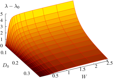
Figure 3: Growth rate characterizing stability of the global mode mixed by the flow with a stationary vortex (11).

The role of a mixing vortex can be understood in the following way. In the case of a passive advection-diffusion process and for a relatively small molecular diffusivity, the field is trapped by the vortex. In the limit of vanishing diffusivity the field $u$ outside the vortex is blown away, whereas everything inside the vortex is trapped and cannot escape for an infinitely long time, as e.g. in [17]. As a result, a pattern in the form of a cloud arises. Because of diffusion, such pattern is no longer stable and its concentration gradually decays. Hence, under an advection-diffusion process, the cloud exists only for a limited time. However, if we now take into consideration activity, this time is spent by the active field to grow, which is enough to compensate the loss caused by diffusion. Thus, a self-sustained pattern is born, Fig. 4.

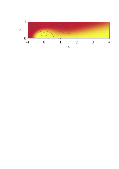
Figure 4: An example of the global mode in the quasi-one-dimensional flow (11) with $V=1$, $W=0.45$, evaluated for $b=1$, $D_{0}=0.01$, $a=1.5$, $p=1$. Higher and lower values of the active field concentration are plotted with the lighter and darker colours, respectively.

Next we calculate the LE for a linearized two-dimensional reaction-advection-diffusion equation (10) with a constant open flow and a superimposed oscillating vortex, described by the stream function

$$\Psi_{2}(x,y,t)=Vy+W\exp[-(x^{2}+y^{2})R^{-2}]\cos(\omega t)\;.$$ (12)

Here we fix $V=1$, $R=1$ and $\omega=2$ and calculate the LE $\Lambda$, see Fig. 5. As before, we plot $\Lambda-\Lambda_{0}$, where $\Lambda_{0}=a-V^{2}/(4D_{0})$ is the LE for a non-mixed flow with $W=0$. Again, the mixing-induced enhancement of field growth is mostly pronounced for small diffusion. In contrast to the previous case the dependence on $W$ is non-monotonic and has a maximum at $W\approx 3$. This is the mixing strength at which a chaotic saddle [1] in the Lagrangean particle trajectories appears. A further increase of the vortex intensity does not lead, however, to a significant growth of the LE.

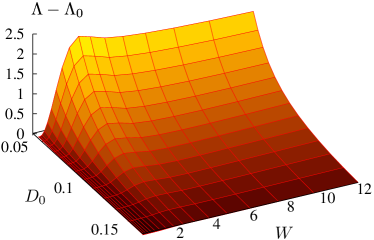
Figure 5: Lyapunov exponent characterizing stability of the global mode mixed by periodically blinking vortex (12).

3 Nonlinear analysis. A universal scaling law

Now we develop a nonlinear theory of the global mode. It is clear that the nonlinear saturation stops the exponential growth of a slightly supercritical linear mode and leads to a nonlinear solution with a finite amplitude. Our aim is to describe the dependence of this amplitude on the deviation from criticality. First we notice, that the very notion of the amplitude is here nontrivial. Indeed, the nonlinear solution looks as in Fig. 1(b) (cf. Fig. 7 below); it saturates to $u=1$ in the downstream direction. However, outside the mixing region the field looks like a solution caused by a localized field source. Thus, we can take the effective intensity of this source $\varepsilon_{eff}$, which is proportional to the characteristic field amplitude in the mixing region $u(0)$ [see relations (2), (3)], as the order parameter of the transition. The deviation from the criticality we will measure with the growth rate $\lambda$, for which holds $\lambda\propto W-W_{cr}$ in the full model (1) or $\lambda\propto D-D_{cr}$ in model (4).

We will consider the simplest possible setup, namely the nonlinear modification of one-dimensional Eq. (5):

$$\frac{\partial u}{\partial t}+V\frac{\partial u}{\partial x}=\frac{\partial}{\partial x}\left[D(x)\frac{\partial u}{\partial x}\right]+au(1-u^{p})\;.$$ (13)

We look for a stationary global mode $u(x)$, and rewrite this equation as the system

$$\frac{dz}{dx} =-z^{2}+\frac{V-\frac{dD(x)}{dx}}{D}z-\frac{a}{D}+\frac{a}{D}u^{p}\;,$$ (14)

$$\frac{du}{dx} =zu\;.$$ (15)

We consider this system separately in two spatial domains. The first, linear region, includes the inflow and the mixing domains (“source” in Fig. 1): $-\infty<x<x_{r}$, where the field $u(x)$ remains small. In the second, outflow region $x_{r}<x<\infty$, the field $u$ further grows (“tail”) and nonlinearly saturates (“plateau”). In the linear region, because of smallness of the field, we can neglect $u^{p}$ in (14), thus we obtain an equation similar to (6). The only difference is that because we look for a stationary solution, in (14) the term $\sim\lambda$ is absent. Near the criticality, where $\lambda$ is small, we can consider this term as a perturbation, therefore the solution of (14) in the linear region is close to the solution of Eq. (6); it has the asymptotic $z\to\mu_{+}$ as $x\to-\infty$. Due to the perturbation term $\propto\lambda$, at the right border of the linear region $z$ deviates from $\mu_{-}$: the deviation $\mu_{-}-z(x_{r})$ is proportional to $\lambda$, and, thus, to $D-D_{cr}$. At $x_{r}$ the field $u$ is small and $u(x_{r})\propto u(0)$.

Next we consider full equations (14), (15) in the nonlinear region $x>x_{r}$. Here the solution should tend as $x\to\infty$ to the saddle fixed point $u=1$, $z=0$. Thus, starting integration from large values of $x$ in the negative direction, we have to follow the stable manifold of this saddle and match this solution at $x=x_{r}$ with the obtained above. Because the value to be matched $z(x_{r})$ is very close to $\mu_{-}$, in the region where the solution $(z,u)$ approaches $(z(x_{r}),u(x_{r}))$ we can write $z^{2}\approx\mu_{-}^{2}-2\mu_{-}\Delta z$ to obtain

$$\frac{d}{dx}\Delta z=(\mu_{+}-\mu_{-})\Delta z-\frac{a}{D}u^{p}(x_{r})e^{p\mu_{-}(x-x_{r})}\;.$$ (16)

Here, since $\Delta z=\mu_{-}-z(x)$ is small, we have approximated the solution of (15) as $u\approx u(x_{r})e^{\mu_{-}(x-x_{r})}$. Because linear inhomogeneous Eq. (16) is solved in the negative in $x$ direction, the solution follows the slowest exponent: $\Delta z\propto\exp[\gamma(x-x_{r})]$, where $\gamma=\min(\mu_{+}-\mu_{-},p\mu_{-})$.

At the criticality, the region of validity of the exponential solution $\Delta z\propto\exp[\gamma(x-x_{r})]$ becomes very large. Thus it is dominant for small deviations from criticality $\lambda$, therefore we can estimate the coordinate $x_{s}$ at which the field $u$ saturates (i.e., we reach the state $u\approx 1$ and $z\approx 0$) from the relations above: from $-\mu_{-}\approx(z(x_{r})-\mu_{-})e^{\gamma(x_{s}-x_{r})}$ it follows $(x_{s}-x_{r})\approx-\gamma^{-1}\ln(\mu_{-}-z(x_{r}))$. Substituting this in the expression for $u(x)$, we obtain $u(x_{r})\propto(\mu_{-}-z(x_{r}))^{\mu_{-}/\gamma}$. Now we take into account that $\mu_{-}-z(x_{r})\propto D-D_{cr}$, and, because the evolution of $u$ in the interval $0<x<x_{r}$ only weakly depends on the criticality, $\varepsilon_{eff}=u(0)\propto u(x_{r})$. The final expression for the scaling law of the amplitude of the global mode thus reads

$$\varepsilon_{eff}\propto\lambda^{\beta}\;,\qquad\beta=\frac{\mu_{-}}{\gamma}=\max\left(\frac{\mu_{-}}{\mu_{+}-\mu_{-}},\frac{1}{p}\right)\;.$$ (17)

The critical index $\beta$ depends only on the nonlinearity index $p$ and on the dimensionless velocity $v=V/V_{f}$:

$$\beta=\left\{\begin{array}[]{ll}p^{-1}&\mbox{if}\;\;v>\frac{2+p}{2\sqrt{1+p}}\;,\\ \frac{v-\sqrt{v^{2}-1}}{2\sqrt{v^{2}-1}}&\mbox{if}\;\;1<v<\frac{2+p}{2\sqrt{1+p}}\;.\end{array}\right.$$ (18)

This main result of our letter can be physically interpreted as follows. The exponent $\beta$ is determined solely by the nonlinearity index $p$ if the throughflow velocity is much larger than the front velocity ($v$ large). Here the field in the plateau domain (see Fig. 1) is effectively uncoupled from the source, and the saturation of the instability is due to the local nonlinearity at the source. For a small throughflow velocity ($v$ close to one) the plateau state interacts with the source via the tail. Due to this “remote control,” the field at the source is saturated more efficiently than due to nonlinearity, here the exponent $\beta$ is determined solely by the form of the tail, which depends on the velocities ratio $v$.

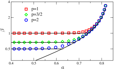
Figure 6: The critical exponent $\beta$ calculated for the model (1) (symbols), compared with theoretical prediction (18) (lines). One can clearly see the crossover between two regimes of the field saturation in dependence on parameter $a$, the latter is related to $v$ in (18) via $v\sim a^{-1/2}$.

Below we check formula (18) with direct numerical simulations of model (1). A stationary vortex (12) with $\omega=0$ and $R=1$ was imposed on a constant flow with $V=1$. Keeping the diffusion constant fixed $D_{0}=0.3$, for different field growth rates $a$ we have found, from the linearized equations, the critical vortex intensities $W_{cr}$ at which the global mode becomes first unstable. Then we solved full nonlinear equations close to criticality and found the exponent $\beta$ according to (17). The stationary problem was solved with a finite difference method in a domain $0\leq x\leq 60$, $0\leq y\leq 40$ with periodic boundary conditions in $y$ and conditions $u(0)=0$, $\frac{\partial u}{\partial x}(60)=0$. The results are presented in Fig. 6, they are in very good agreement with the theoretical prediction (17), (18). Figure 7 shows the example of the stationary mode appearing beyond the instability threshold. A similar analysis performed for the quasi-one-dimensional flow (11) also provides very good agreement with formula (18).

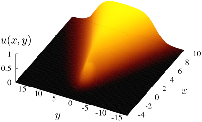
Figure 7: The active field behind a vortex with $W=4$ placed at $x=y=0$, for $V=1$, $a=0.5$, $D_{0}=0.3$, $p=2$.

4 Conclusions

We have described the mixing-induced transition from a convectively unstable active field in an open flow to a persistent global mode. Our theoretical approach bases on the representation of the mixing region as a domain with locally enhanced effective diffusion. For a nonlinear regime close to criticality we have derived the critical exponent $\beta$ (18) that depends only on two parameters of the system: the dimensionless flow velocity $v$ normalized by that of the front, and the nonlinearity index $p$. For large velocities the critical exponent depends only on the system’s nonlinearity, which means a local in space saturation of the instability. For small velocities the exponent is a function of velocity, here the growing downstream tail of the active field imposes the saturation. Notably, this prediction of the one-dimensional theory is in a good accordance with two-dimensional calculations. The obtained results are independent of the geometry and the nature of the mixing region and for these reasons are expected in different systems and at different scales. The generic nature of our findings indicates that turbulent mixing can play a key role in open flows that involve active chemical and biological processes.

References

References

- [1] Tél T, de Moura A, Grebogi C and Károlyi G 2005 Phys. Rep. 413, 91–196
- [2] Kuznetsov S P, Mosekilde E, Dewel G and Borckmans P 1997 J Chem. Phys. 106, 7609–7616
- [3] McGraw P N and Menzinger M 2003 Phys. Rev. E 68, 066122
- [4] Sandulescu M, Hernández-García E, López C and Feudel U 2006 Tellus A 58, 605–615
- [5] Sibly R M, Barker D, Denham M C, Hone J and Pagel M 2005 Science 309, 607–610
- [6] Murray J D 1993 Mathematical Biology (Berlin: Springer)
- [7] Huisman J, Pham Thi N N, Karl D M and Sommeijer B 2006 Nature 439, 322–325
- [8] Leconte M, Martin J, Rakotomalala N and Salin D 2003 Phys. Rev. Lett. 90, 128302
- [9] van Saarloos 2003 Phys. Rep. 386, 29–222
- [10] Chomaz J M, Huerre P and Redekopp L G 1988 Phys. Rev. Lett. 60, 25–28
- [11] Couairon A and Chomaz J-M 1997 Physica D 108, 236–276
- [12] Tobias S M, Proctor M R E and Knobloch E 1998 Physica D 113, 43–72
- [13] Dimotakis P E 2005 Annu. Rev. Fluid Mech. 37, 329–356
- [14] Nelson D R and Shnerb N M 1998 Phys. Rev. E 58, 1383–1403
- [15] Dahmen K A, Nelson D R and Shnerb N M 2000 J. Math. Biol. 41, 1–23
- [16] Pikovsky A and Popovych O 2003 Europhys. Lett. 61, 625–631
- [17] Lyubimov D V, Straube A V and Lyubimova T P 2005 Phys. Fluids 17, 063302