Regularized Multivariate Regression for Identifying Master Predictors with Application to Integrative Genomics Study of Breast Cancer

Abstract

In this paper, we propose a new method remMap — REgularized Multivariate regression for identifying MAster Predictors — for fitting multivariate response regression models under the high-dimension-low-sample-size setting. remMap is motivated by investigating the regulatory relationships among different biological molecules based on multiple types of high dimensional genomic data. Particularly, we are interested in studying the influence of DNA copy number alterations on RNA transcript levels. For this purpose, we model the dependence of the RNA expression levels on DNA copy numbers through multivariate linear regressions and utilize proper regularization to deal with the high dimensionality as well as to incorporate desired network structures. Criteria for selecting the tuning parameters are also discussed. The performance of the proposed method is illustrated through extensive simulation studies. Finally, remMap is applied to a breast cancer study, in which genome wide RNA transcript levels and DNA copy numbers were measured for 172 tumor samples. We identify a trans-hub region in cytoband 17q12-q21, whose amplification influences the RNA expression levels of more than $30$ unlinked genes. These findings may lead to a better understanding of breast cancer pathology.

Key words: sparse regression, MAP(MAster Predictor) penalty, DNA copy number alteration, RNA transcript level, v-fold cross validation.

1 Introduction

In a few recent breast cancer cohort studies, microarray expression experiments and array CGH (comparative genomic hybridization) experiments have been conducted for more than $170$ primary breast tumor specimens collected at multiple cancer centers Sorlie:2001,Sorlie:2003,Zhao:2004,Kapp:2006,Bergamaschi:2006,Langerod:2007,Bergamaschi:2008. The resulting RNA transcript levels (from microarray expression experiments) and DNA copy numbers (from CGH experiments) of about $20K$ genes/clones across all the tumor samples were then used to identify useful molecular markers for potential clinical usage. While useful information has been revealed by analyzing expression arrays alone or CGH arrays alone, careful integrative analysis of DNA copy numbers and expression data are necessary as these two types of data provide complimentary information in gene characterization. Specifically, RNA data give information on genes that are over/under-expressed, but do not distinguish primary changes driving cancer from secondary changes resulting from cancer, such as proliferation rates and differentiation state. On the other hand, DNA data give information on gains and losses that are drivers of cancer. Therefore, integrating DNA and RNA data helps to discern more subtle (yet biologically important) genetic regulatory relationships in cancer cells Pollack:2002.

It is widely agreed that variations in gene copy numbers play an important role in cancer development through altering the expression levels of cancer-related genes Albertson:2003. This is clear for cis-regulations, in which a gene’s DNA copy number alteration influences its own RNA transcript level Hyman:2002,Pollack:2002. However, DNA copy number alterations can also alter in trans the RNA transcript levels of genes from unlinked regions, for example by directly altering the copy number and expression of transcriptional regulators, or by indirectly altering the expression or activity of transcriptional regulators, or through genome rearrangements affecting cis-regulatory elements. The functional consequences of such trans-regulations are much harder to establish, as such inquiries involve assessment of a large number of potential regulatory relationships. Therefore, to refine our understanding of how these genome events exert their effects, we need new analytical tools that can reveal the subtle and complicated interactions among DNA copy numbers and RNA transcript levels. Knowledge resulting from such analysis will help shed light on cancer mechanisms.

The most straightforward way to model the dependence of RNA levels on DNA copy numbers is through a multivariate response linear regression model with the RNA levels being responses and the DNA copy numbers being predictors. While the multivariate linear regression is well studied in statistical literature, the current problem bears new challenges due to (i) high-dimensionality in terms of both predictors and responses; (ii) the interest in identifying master regulators in genetic regulatory networks; and (iii) the complicated relationships among response variables. Thus, the naive approach of regressing each response onto the predictors separately is unlikely to produce satisfactory results, as such methods often lead to high variability and over-fitting. This has been observed by many authors, for example,  Breiman:1997 show that taking into account of the relation among response variables helps to improve the overall prediction accuracy. More recently,  Kim:2008 propose a new statistical framework to explicitly incorporate the relationships among responses by assuming the linked responses depend on the predictors in a similar way. The authors show that this approach helps to select relevant predictors when the above assumption holds.

When the number of predictors is moderate or large, model selection is often needed for prediction accuracy and/or model interpretation. Standard model selection tools in multiple regression such as AIC and forward stepwise selection have been extended to multivariate linear regression models  Bedrick:1994,Fujikoshi:1997,Lutz:2006. More recently, sparse regularization schemes have been utilized for model selection under the high dimensional multivariate regression setting. For example,  Turlach:2005 propose to constrain the coefficient matrix of a multivariate regression model to lie within a suitable polyhedral region. Lutz:2006 propose an $L_{2}$ multivariate boosting procedure. Obozinskiy:2008 propose to use a $\ell_{1}/\ell_{2}$ regularization to identify the union support set in the multivariate regression. Moreover, Brown et al. (1998, 1999, 2002) introduce a Bayesian framework to model the relation among the response variables when performing variable selection for multivariate regression. Another way to reduce the dimensionality is through factor analysis. Related work includes Izenman:1975, Frank:1993, Reinsel:1998, YuanMulti:2007 and many others.

For the problem we are interested in here, the dimensions of both predictors and responses are large (compared to the sample size). Thus in addition to assuming that only a subset of predictors enter the model, it is also reasonable to assume that a predictor may affect only some but not all responses. Moreover, in many real applications, there often exist a subset of predictors which are more important than other predictors in terms of model building and/or scientific interest. For example, it is widely believed that genetic regulatory relationships are intrinsically sparse Jeong:2001,Gardner:2003. At the same time, there exist master regulators — network components that affect many other components, which play important roles in shaping the network functionality. Most methods mentioned above do not take into account the dimensionality of the responses, and thus a predictor/factor influences either all or none responses, e.g., Turlach:2005, YuanMulti:2007, the $L_{2}$ row boosting by Lutz:2006, and the $\ell_{1}/\ell_{2}$ regularization by Obozinskiy:2008. On the other hand, other methods only impose a sparse model, but do not aim at selecting a subset of predictors, e.g., the $L_{2}$ boosting by Lutz:2006. In this paper, we propose a novel method remMap — REgularized Multivariate regression for identifying MAster Predictors, which takes into account both aspects. remMap uses an $\ell_{1}$ norm penalty to control the overall sparsity of the coefficient matrix of the multivariate linear regression model. In addition, remMap imposes a “group” sparse penalty, which in essence is the same as the “group lasso” penalty proposed by Bakin:1999, Antoniadis:2001, YuanLin:2006, Zhao:2006 and Obozinskiy:2008 (see more discussions in Section 2). This penalty puts a constraint on the $\ell_{2}$ norm of regression coefficients for each predictor, which controls the total number of predictors entering the model, and consequently facilitates the detection of master predictors. The performance of the proposed method is illustrated through extensive simulation studies.

We apply the remMap method on the breast cancer data set mentioned earlier and identify a significant trans-hub region in cytoband 17q12-q21, whose amplification influences the RNA levels of more than 30 unlinked genes. These findings may shed some light on breast cancer pathology. We also want to point out that analyzing CGH arrays and expression arrays together reveals only a small portion of the regulatory relationships among genes. However, it should identify many of the important relationships, i.e., those reflecting primary genetic alterations that drive cancer development and progression. While there are other mechanisms to alter the expression of master regulators, for example by DNA mutation or methylation, in most cases one should also find corresponding DNA copy number changes in at least a subset of cancer cases. Nevertheless, because we only identify the subset explainable by copy number alterations, the words “regulatory network” (“master regulator”) used in this paper will specifically refer to the subnetwork (hubs of the subnetwork) whose functions change with DNA copy number alterations, and thus can be detected by analyzing CGH arrays together with expression arrays.

The rest of the paper is organized as follows. In Section 2, we describe the remMap model, its implementation and criteria for tuning. In Section 3, the performance of remMap is examined through extensive simulation studies. In Section 4, we apply the remMap method on the breast cancer data set. We conclude the paper with discussions in Section 5. Technical details are provided in the supplementary material.

2 Method

2.1 Model

Consider multivariate regression with $Q$ response variables $y_{1},\cdots,y_{Q}$ and $P$ prediction variables $x_{1},\cdots,x_{P}$:

$$y_{q}=\sum_{p=1}^{P}x_{p}\beta_{pq}+\epsilon_{q},\quad q=1,\cdots,Q,$$ (1)

where the error terms $\epsilon_{1},\cdots,\epsilon_{Q}$ have a joint distribution with mean $0$ and covariance $\mathbf{\Sigma}_{\epsilon}$. The primary goal of this paper is to identify non-zero entries in the $P\times Q$ coefficient matrix $\mathbf{B}=(\beta_{pq})$ based on $N$ i.i.d samples from the above model. Under normality assumptions, $\beta_{pq}$ can be interpreted as proportional to the conditional correlation $\text{Cor}(y_{q},x_{p}|x_{-(p)})$, where $x_{-(p)}:=\{x_{p^{\prime}}:1\leq p^{\prime}\neq p\leq P\}$. In the following, we use $Y_{q}=(y^{1}_{q},\cdots,y^{N}_{q})^{T}$ and $X_{p}=(x^{1}_{p},\cdots,x^{N}_{p})^{T}$ to denote the sample of the $q^{th}$ response variable and that of the $p^{th}$ prediction variable, respectively. We also use $\mathbf{Y}=(Y_{1}:\cdots:Y_{Q})$ to denote the $N\times Q$ response matrix, and use $\mathbf{X}=(X_{1}:\cdots:X_{P})$ to denote the $N\times P$ prediction matrix.

In this paper, we shall focus on the cases where both $Q$ and $P$ are larger than the sample size $N$. For example, in the breast cancer study discussed in Section 4, the sample size is $172$, while the number of genes and the number of chromosomal regions are on the order of a couple of hundreds (after pre-screening). When $P>N$, the ordinary least square solution is not unique, and regularization becomes indispensable. The choice of suitable regularization depends heavily on the type of data structure we envision. In recent years, $\ell_{1}$-norm based sparsity constraints such as lasso  Lasso:1996 have been widely used under such high-dimension-low-sample-size settings. This kind of regularization is particularly suitable for the study of genetic pathways, since genetic regulatory relationships are widely believed to be intrinsically sparse Jeong:2001,Gardner:2003. In this paper, we impose an $\ell_{1}$ norm penalty on the coefficient matrix $\mathbf{B}$ to control the overall sparsity of the multivariate regression model. In addition, we put constraints on the total number of predictors entering the model. This is achieved by treating the coefficients corresponding to the same predictor (one row of $\mathbf{B}$) as a group, and then penalizing their $\ell_{2}$ norm. A predictor will not be selected into the model if the corresponding $\ell_{2}$ norm is shrunken to $0$. Thus this penalty facilitates the identification of master predictors — predictors which affect (relatively) many response variables. This idea is motivated by the fact that master regulators exist and are of great interest in the study of many real life networks including genetic regulatory networks. Specifically, for model (1), we propose the following criterion

$$L(\mathbf{B};\lambda_{1},\lambda_{2})=\frac{1}{2}||\mathbf{Y}-\sum_{p=1}^{P}X_{p}B_{p}||^{2}_{F}+\lambda_{1}\sum_{p=1}^{P}||C_{p}\cdot B_{p}||_{1}+\lambda_{2}\sum_{p=1}^{P}||C_{p}\cdot B_{p}||_{2},$$ (2)

where $C_{p}$ is the $p$th row of $\mathbf{C}=(c_{pq})=(C_{1}^{T}:\cdots:C_{P}^{T})^{T}$, which is a pre-specified $P\times Q$ 0-1 matrix indicating the coefficients on which penalization is imposed; $B_{p}$ is the $p^{th}$ row of $\mathbf{B}$; $||\cdot||_{F}$ denotes the Frobenius norm of matrices; $||\cdot||_{1}$ and $||\cdot||_{2}$ are the $\ell_{1}$ and $\ell_{2}$ norms for vectors, respectively; and “$\cdot$” stands for Hadamard product (that is, entry-wise multiplication). The indicator matrix $\mathbf{C}$ is pre-specified based on prior knowledge: if we know in advance that predictor $x_{p}$ affects response $y_{q}$, then the corresponding regression coefficient $\beta_{pq}$ will not be penalized and we set $c_{pq}=0$ (see Section 4 for an example). When there is no such prior information, $\mathbf{C}$ can be simply set to a constant matrix $c_{pq}\equiv 1$. Finally, an estimate of the coefficient matrix $\mathbf{B}$ is $\widehat{\mathbf{B}}(\lambda_{1},\lambda_{2}):=\arg\min_{\mathbf{B}}L(\mathbf{B};\lambda_{1},\lambda_{2})$.

In the above criterion function, the $\ell_{1}$ penalty induces the overall sparsity of the coefficient matrix $\mathbf{B}$. The $\ell_{2}$ penalty on the row vectors $C_{p}\cdot B_{p}$ induces row sparsity of the product matrix $\mathbf{C}\cdot\mathbf{B}$. As a result, some rows are shrunken to be entirely zero (Theorem 1). Consequently, predictors which affect relatively more response variables are more likely to be selected into the model. We refer to the combined penalty in equation (2) as the MAP (MAster Predictor) penalty. We also refer to the proposed estimator $\widehat{\mathbf{B}}(\lambda_{1},\lambda_{2})$ as the remMap (REgularized Multivariate regression for identifying MAster Predictors) estimator. Note that, the $\ell_{2}$ penalty is a special case (with $\alpha=2$) of the more general penalty form: $\sum_{p=1}^{P}||C_{p}\cdot B_{p}||_{\alpha}$, where $||v||_{\alpha}:=(\sum_{q=1}^{Q}|v_{q}|^{\alpha})^{\frac{1}{\alpha}}$ for a vector $v\in\mathcal{R}^{Q}$ and $\alpha>1$. In  Turlach:2005, a penalty with $\alpha=\infty$ is used to select a common subset of prediction variables when modeling multivariate responses. In Yuan et al. (2007), a constraint with $\alpha=2$ is applied to the loading matrix in a multivariate linear factor regression model for dimension reduction. In  Obozinskiy:2008, the same constraint is applied to identify the union support set in the multivariate regression. In the case of multiple regression, a similar penalty corresponding to $\alpha=2$ is proposed by Bakin:1999 and by YuanLin:2006 for the selection of grouped variables, which corresponds to the blockwise additive penalty in Antoniadis:2001 for wavelet shrinkage. Zhao:2006 propose the penalty with a general $\alpha>1$. However, none of these methods takes into account the high dimensionality of response variables and thus predictors/factors are simultaneously selected for all responses. On the other hand, by combining the $\ell_{2}$ penalty and the $\ell_{1}$ penalty together in the MAP penalty, the remMap model not only selects a subset of predictors, but also limits the influence of the selected predictors to only some (but not necessarily all) response variables. Thus, it is more suitable for the cases when both the number of predictors and the number of responses are large. Lastly, we also want to point out a difference between the MAP penalty and the ElasticNet penalty proposed by  Zou:2005, which combines the $\ell_{1}$ norm penalty with the squared $\ell_{2}$ norm penalty. The ElasticNet penalty aims to encourage a group selection effect for highly correlated predictors under the multiple regression setting. However, the squared $\ell_{2}$ norm itself does not induce sparsity and thus is intrinsically different from the $\ell_{2}$ norm penalty discussed above.

In Section 3, we use extensive simulation studies to illustrate the effects of the MAP penalty. We compare the remMap method with two alternatives: (i) the joint method which only utilizes the $\ell_{1}$ penalty, that is $\lambda_{2}=0$ in (2); (ii) the sep method which performs $Q$ separate lasso regressions. We find that, if there exist large hubs (master predictors), remMap performs much better than joint in terms of identifying the true model; otherwise, the two methods perform similarly. This suggests that the “simultaneous” variable selection enhanced by the $\ell_{2}$ penalty pays off when there exist a small subset of “important” predictors, and it costs little when such predictors are absent. In addition, both remMap and joint methods impose sparsity of the coefficient matrix as a whole. This helps to borrow information across different regressions corresponding to different response variables, and thus incorporates the relationships among response variables into the model. It also amounts to a greater degree of regularization, which is usually desirable for the high-dimension-low-sample-size setting. On the other hand, the sep method controls sparsity for each individual regression separately and thus is subject to high variability and over-fitting. As can be seen by the simulation studies (Section 3), this type of “joint” modeling greatly improves the model efficiency. This is also noted by other authors including  Turlach:2005,  Lutz:2006 and  Obozinskiy:2008.

2.2 Model Fitting

In this section, we propose an iterative algorithm for solving the remMap estimator $\widehat{\mathbf{B}}(\lambda_{1},\lambda_{2})$. This is a convex optimization problem when the two tuning parameters are not both zero, and thus there exists a unique solution. We first describe how to update one row of $\mathbf{\mathbf{B}}$, when all other rows are fixed.

Theorem 1

Given $\{B_{p}\}_{p\not=p_{0}}$ in (2), the solution for $\min_{B_{p_{0}}}L(\mathbf{B};\lambda_{1},\lambda_{2})$ is given by $\widehat{B}_{p_{0}}=(\widehat{\beta}_{p_{0},1},\cdots,\widehat{\beta}_{p_{0},Q})$ which satisfies: for $1\leq q\leq Q$

• If $c_{p_{0},q}=0$, $\widehat{\beta}_{p_{0},q}=X_{p_{0}}^{T}\widetilde{Y}_{q}/\|X_{p_{0}}\|_{2}^{2}$ (OLS), where $\widetilde{Y}_{q}=Y_{q}-\sum_{p\neq p_{0}}X_{p}\beta_{pq}$;

• If $c_{p_{0},q}=1$,

  $$\widehat{\beta}_{p_{0},q}=\left\{\begin{array}[]{ll}0,&{\textrm{i}f}~{}\|\widehat{B}_{p_{0}}^{{\textrm{l}asso}}\|_{2,C}=0;\\ \left(1-\frac{\lambda_{2}}{\|\widehat{\mathbf{B}}_{p_{0}}^{{\textrm{l}asso}}\|_{2,C}\cdot\|X_{p_{0}}\|_{2}^{2}}\right)_{+}\widehat{\beta}_{p_{0},q}^{\rm{lasso}},&\rm{otherwise,}\end{array}\right.$$ (5)

where

$$||\widehat{B}_{p_{0}}^{\rm{lasso}}||_{2,C}:=\left\{\sum_{q=1}^{Q}c_{p_{0},q}(\widehat{\beta}_{p_{0},q}^{\rm{lasso}})^{2}\right\}^{1/2},$$

and

$$\widehat{\beta}_{p_{0},q}^{\rm{lasso}}=\left\{\begin{array}[]{ll}X_{p_{0}}^{T}\widetilde{Y}_{q}/\|X_{p_{0}}\|_{2}^{2},&{\textrm{i}f}~{}c_{p_{0},q}=0;\\ \left(|X_{p_{0}}^{T}\widetilde{Y}_{q}|-\lambda_{1}\right)_{+}\frac{{\textrm{s}ign}\left(X_{p_{0}}^{T}\widetilde{Y}_{q}\right)}{\|X_{p_{0}}\|_{2}^{2}},&{\textrm{i}f}~{}c_{p_{0},q}=1.\end{array}\right.$$ (8)

The proof of Theorem 1 is given in the supplementary material (Appendix A).

Theorem 1 says that, when estimating the $p_{0}^{th}$ row of the coefficient matrix $\mathbf{B}$ with all other rows fixed: if there is a pre-specified relationship between the $p_{0}^{th}$ predictor and the $q^{th}$ response (i.e., $c_{p_{0},q}=0$), the corresponding coefficient $\beta_{p_{0},q}$ is estimated by the (univariate) ordinary least square solution (OLS) using current responses $\widetilde{Y}_{q}$; otherwise, we first obtain the lasso solution $\widehat{\beta}_{p_{0},q}^{\rm{lasso}}$ by the (univariate) soft shrinkage of the OLS solution (equation (8)), and then conduct a group shrinkage of the lasso solution (equation (5)). From Theorem 1, it is easy to see that, when the design matrix $\mathbf{X}$ is orthonormal: $\mathbf{X}^{T}\mathbf{X}=I_{p}$ and $\lambda_{1}=0$, the remMap method amounts to selecting variables according to the $\ell_{2}$ norm of their corresponding OLS estimates.

Theorem 1 naturally leads to an algorithm which updates the rows of $\mathbf{B}$ iteratively until convergence. In particular, we adopt the active-shooting idea proposed by space:2008 and  Friedman:2008, which is a modification of the shooting algorithm proposed by  Fu:1998 and also  Friedman:2007 among others. The algorithm proceeds as follows:

• Initial step: for $p=1,...,P$; $q=1,...,Q$,

  $$\widehat{\beta}_{p,q}^{0}=\left\{\begin{array}[]{lll}X_{p}^{T}Y_{q}/\|X_{p}\|_{2}^{2},&\rm{if}&c_{p,q}=0;\\ \left(|X_{p}^{T}Y_{q}|-\lambda_{1}\right)_{+}\frac{{\textrm{s}ign}\left(X_{p}^{T}Y_{q}\right)}{\|X_{p}\|_{2}^{2}},&\rm{if}&c_{p,q}=1.\end{array}\right.$$ (11)

• Define the current active-row set $\Lambda=\{p:\textrm{ current }||\widehat{B}_{p}||_{2,C}\neq 0\}$.

  • For each $p\in\Lambda$, update $\widehat{B}_{p}$ with all other rows of $\mathbf{B}$ fixed at their current values according to Theorem 1.

  • Repeat (2.1) until convergence is achieved on the current active-row set.

• For $p=1\textrm{ to }P$, update $\widehat{B}_{p}$ with all other rows of $\mathbf{B}$ fixed at their current values according to Theorem 1. If no $\widehat{B}_{p}$ changes during this process, return the current $\widehat{\mathbf{B}}$ as the final estimate. Otherwise, go back to step 2.

It is clear that the computational cost of the above algorithm is in the order of $O(NPQ)$.

2.3 Tuning

In this section, we discuss the selection of the tuning parameters $(\lambda_{1},\lambda_{2})$ by v-fold cross validation. To perform the v-fold cross validation, we first partition the whole data set into $V$ non-overlapping subsets, each consisting of approximately $1/V$ fraction of total samples. Denote the $i^{th}$ subset as $D^{(i)}=(\mathbf{Y}^{(i)},\mathbf{X}^{(i)})$, and its complement as $D^{-(i)}=(\mathbf{Y}^{-(i)},\mathbf{X}^{-(i)})$. For a given $(\lambda_{1},\lambda_{2})$, we obtain the remMap estimate: $\widehat{\mathbf{B}}^{(i)}(\lambda_{1},\lambda_{2})=(\widehat{\beta}_{pq}^{(i)})$ based on the $i^{th}$ training set $D^{-(i)}$. We then obtain the ordinary least square estimates $\widehat{\mathbf{B}}_{\rm{ols}}^{(i)}(\lambda_{1},\lambda_{2})=(\widehat{\beta}_{\textrm{ols},pq}^{(i)})$ as follows: for $1\leq q\leq Q$, define $S_{q}=\{p:1\leq p\leq P,\widehat{\beta}_{pq}^{(i)}\neq 0\}$. Then set $\widehat{\beta}_{\textrm{ols},pq}^{(i)}=0$ if $p\notin S_{q}$; otherwise, define $\{\widehat{\beta}_{\textrm{ols},pq}^{(i)}:p\in S_{q}\}$ as the ordinary least square estimates by regressing $Y_{q}^{-(i)}$ onto $\{X_{p}^{-(i)}:p\in S_{q}\}$. Finally, prediction error is calculated on the test set $D^{(i)}$:

$$\texttt{remMap.cv}_{i}(\lambda_{1},\lambda_{2}):=||\mathbf{Y}^{(i)}-\mathbf{X}^{(i)}\widehat{\mathbf{B}}_{\rm{ols}}^{(i)}(\lambda_{1},\lambda_{2})||^{2}_{2}.$$ (12)

The v-fold cross validation score is then defined as

$$\texttt{remMap.cv}(\lambda_{1},\lambda_{2})=\sum_{i=1}^{V}\texttt{remMap.cv}_{i}(\lambda_{1},\lambda_{2}).$$ (13)

The reason for using OLS estimates in calculating the prediction error is because the true model is assumed to be sparse. As noted by lars, when there are many noise variables, using shrunken estimates in the cross validation criterion often results in over fitting. Similar results are observed in our simulation studies: if in (12) and (13), the shrunken estimates are used, the selected models are all very big which result in large numbers of false positive findings. In addition, we also try AIC and GCV for tuning and both criteria result in over fitting as well. These results are not reported in the next section due to space limitation.

In order to further control the false positive findings, we propose a method called cv.vote. The idea is to treat the training data from each cross-validation fold as a “bootstrap” sample. Then variables being consistently selected by many cross validation folds should be more likely to appear in the true model than the variables being selected only by few cross validation folds. Specifically, for $1\leq p\leq P$ and $1\leq q\leq Q$, define

$$s_{pq}(\lambda_{1},\lambda_{2})=\left\{\begin{array}[]{ll}1,&\textrm{ if }\sum_{i=1}^{V}I(\widehat{\beta}_{pq}^{(i)}(\lambda_{1},\lambda_{2})\neq 0)>V_{a};\\ 0,&\textrm{ otherwise}.\end{array}\right.$$ (16)

where $V_{a}$ is a pre-specified integer. We then select edge $(p,q)$ if $s_{pq}(\lambda_{1},\lambda_{2})=1$. In the next section, we use $V_{a}=5$ and thus cv.vote amounts to a “majority vote” procedure. Simulation studies in Section 3 suggest that, cv.vote can effectively decrease the number of false positive findings while only slightly increase the number of false negatives.

An alternative tuning method is by a BIC criterion. Compared to v-fold cross validation, BIC is computationally cheaper. However it requires much more assumptions. In particular, the BIC method uses the degrees of freedom of each remMap model which is difficult to estimate in general. In the supplementary material, we derive an unbiased estimator for the degrees of freedom of the remMap models when the predictor matrix $\mathbf{X}$ has orthogonal columns (Theorem 2 of Appendix B in the supplementary materials). In Section 3, we show by extensive simulation studies that, when the correlations among the predictors are complicated, this estimator tends to select very small models. For more details see the supplementary material, Appendix B.

3 Simulation

In this section, we investigate the performance of the remMap model and compare it with two alternatives: (i) the joint model with $\lambda_{2}=0$ in (2); (ii) the sep model which performs $Q$ separate lasso regressions. For each model, we consider three tuning strategies, which results in nine methods in total:

1. remMap.cv, joint.cv, sep.cv:    The tuning parameters are selected through 10-fold cross validation;

2. remMap.cv.vote, joint.cv.vote, sep.cv.vote:    The cv.vote procedure with $V_{a}=5$ is applied to the models resulted from the corresponding $*$.cv approaches;

3. remMap.bic, joint.bic, sep.bic:     The tuning parameters are selected by a BIC criterion. For remMap.bic and joint.bic, the degrees of freedom are estimated according to equation (S-9) in Appendix B of the supplementary material; for sep.bic, the degrees of freedom of each regression is estimated by the total number of selected predictors  Zou:2007.

We simulate data as follows. Given $(N,P,Q)$, we first generate the predictors $(x_{1},\cdots,x_{P})^{T}\sim~{}{\textrm{N}ormal}_{P}(0,\mathbf{\Sigma}_{X})$, where $\mathbf{\Sigma}_{X}$ is the predictor covariance matrix (for simulations 1 and 2, $\mathbf{\Sigma}_{X}(p,p^{\prime}):=\rho_{x}^{|p-p^{\prime}|}$). Next, we simulate a $P\times Q$ 0-1 adjacency matrix $\mathbf{A}$, which specifies the topology of the network between predictors and responses, with $\mathbf{A}(p,q)=1$ meaning that $x_{p}$ influences $y_{q}$, or equivalently $\beta_{pq}\neq 0$. In all simulations, we set $P=Q$ and the diagonals of $\mathbf{A}$ equal to one, which is viewed as prior information (thus the diagonals of $\mathbf{C}$ are set to zero). This aims to mimic cis-regulations of DNA copy number alternations on its own expression levels. We then simulate the $P\times Q$ regression coefficient matrix $\mathbf{B}=(\beta_{pq})$ by setting $\beta_{pq}=0$, if $\mathbf{A}(p,q)=0$; and $\beta_{pq}\sim{\rm Uniform}([-5,-1]\cup[1,5])$, if $\mathbf{A}(p,q)=1$. After that, we generate the residuals $(\epsilon_{1},\cdots,\epsilon_{Q})^{T}\sim~{}{\textrm{N}ormal}_{Q}(0,\mathbf{\Sigma}_{\epsilon})$, where $\mathbf{\Sigma}_{\epsilon}(q,q^{\prime})=\sigma^{2}_{\epsilon}\rho_{\epsilon}^{|q-q^{\prime}|}$. The residual variance $\sigma^{2}_{\epsilon}$ is chosen such that the average signal to noise ratio equals to a pre-specified level $s$. Finally, the responses $(y_{1},\cdots,y_{Q})^{T}$ are generated according to model (1). Each data set consists of $N$ i.i.d samples of such generated predictors and responses. For all methods, predictors and responses are standardized to have (sample) mean zero and standard deviation one before model fitting. Results reported for each simulation setting are averaged over $25$ independent data sets.

For all simulation settings, $\mathbf{C}=(c_{pq})$ is taken to be $c_{pq}=0$, if $p=q$; and $c_{pq}=1$, otherwise. Our primary goal is to identify the trans-edges — the predictor-response pairs $(x_{p},y_{q})$ with $\mathbf{A}(p,q)=1$ and $\mathbf{C}(p,q)=1$, i.e., the edges that are not pre-specified by the indicator matrix $\mathbf{C}$. Thus, in the following, we report the number of false positive detections of trans-edges (FP) and the number of false negative detections of trans-edges (FN) for each method. We also examine these methods in terms of predictor selection. Specifically, a predictor is called a cis-predictor if it does not have any trans-edges; otherwise it is called a trans-predictor. Moreover, we say a false positive trans-predictor (FPP) occurs if a cis-predictor is incorrectly identified as a trans-predictor; we say a false negative trans-predictor (FNP) occurs if it is the other way around.

Simulation I

We first assess the performances of the nine methods under various combinations of model parameters. Specifically, we consider: $P=Q=400,600,800$; $s=0.25,0.5,0.75$; $\rho_{x}=0,0.4,0.8$; and $\rho_{\epsilon}=0,0.4,0.8$. For all settings, the sample size $N$ is fixed at $200$. The networks (adjacency matrices $\mathbf{A}$) are generated with $5$ master predictors (hubs), each influencing $20\sim 40$ responses; and all other predictors are cis-predictors. We set the total number of tran-edges to be $132$ for all networks. Results on trans-edge detection are summarized in Figures 1 and 2. From these figures, it is clear that remMap.cv and remMap.cv.vote perform the best in terms of the total number of false detections (FP+FN), followed by remMap.bic. The three sep methods result in too many false positives (especially sep.cv). This is expected since there are in total $Q$ tuning parameters selected separately, and the relations among responses are not utilized at all. This leads to high variability and over-fitting. The three joint methods perform reasonably well, though they have considerably larger number of false negative detections compared to remMap methods. This is because the joint methods incorporate less information about the relations among the responses caused by the master predictors. Finally, comparing cv.vote to cv, we can see that the cv.vote procedure effectively decreases the false positive detections and only slightly inflates the false negative counts.

As to the impact of different model parameters, signal size $s$ plays an important role for all methods: the larger the signal size, the better these methods perform (Figure 1(a)). Dimensionality $(P,Q)$ also shows consistent impacts on these methods: the larger the dimension, the more false negative detections (Figure 1(b)). With increasing predictor correlation $\rho_{x}$, both remMAP.bic and joint.bic tend to select smaller models, and consequently result in less false positives and more false negatives (Figure 2(a)). This is because when the design matrix $\mathbf{X}$ is further away from orthogonality, (S-9) tends to overestimate the degrees of freedom and consequently smaller models are selected. The residual correlation $\rho_{\epsilon}$ seems to have little impact on joint and sep, and some (though rather small) impacts on remMap (Figure 2(b)). Moreover, remMap performs much better than joint and sep on master predictor selection, especially in terms of the number of false positive trans-predictors (results not shown). This is because the $\ell_{2}$ norm penalty is more effective than the $\ell_{1}$ norm penalty in excluding irrelevant predictors.

Simulation II

In this simulation, we study the performance of these methods on a network without big hubs. The data are generated similarly as before with $P=Q=600$, $N=200$, $s=0.25$, $\rho_{x}=0.4$, and $\rho_{\epsilon}=0$. The network consists of $540$ cis-predictors, and $60$ trans-predictors with $1\sim 4$ trans-edges. This leads to $151$ trans-edges in total. As can be seen from Table 1, remMap methods and joint methods now perform very similarly and both are considerably better than the sep methods. Indeed, under this setting, $\lambda_{2}$ is selected (either by cv or bic) to be small in the remMap model, making it very close to the joint model.

Table 1: Simulation II. Network topology: uniform network with $151$ trans-edges and $60$ trans-predictors. $P=Q=600,N=200$; $s=0.25$; $\rho_{x}=0.4$; $\rho_{\epsilon}=0$.

Method	FP	FN	TF	FPP	FNP
remMap.bic	4.72(2.81)	45.88(4.5)	50.6(4.22)	1.36(1.63)	11(1.94)
remMap.cv	18.32(11.45)	40.56(5.35)	58.88(9.01)	6.52(5.07)	9.2(2)
remMap.cv.vote	2.8(2.92)	50.32(5.38)	53.12(3.94)	0.88(1.26)	12.08(1.89)
joint.bic	5.04(2.68)	52.92(3.6)	57.96(4.32)	4.72(2.64)	9.52(1.66)
joint.cv	16.96(10.26)	46.6(5.33)	63.56(7.93)	15.36(8.84)	7.64(2.12)
joint.cv.vote	2.8(2.88)	56.28(5.35)	59.08(4.04)	2.64(2.92)	10.40(2.08)
sep.bic	78.92(8.99)	37.44(3.99)	116.36(9.15)	67.2(8.38)	5.12(1.72)
sep.cv	240.48(29.93)	32.4(3.89)	272.88(30.18)	179.12(18.48)	2.96(1.51)
sep.cv.vote	171.00(20.46)	33.04(3.89)	204.04(20.99)	134.24(14.7)	3.6(1.50)
FP: false positive; FN: false negative; TF: total false; FPP: false positive trans-predictor;
FNP: false negative trans-predictor. Numbers in the parentheses are standard deviations

Simulation III

In this simulation, we try to mimic the true predictor covariance and network topology in the real data discussed in the next section. We observe that, for chromosomal regions on the same chromosome, the corresponding copy numbers are usually positively correlated, and the magnitude of the correlation decays slowly with genetic distance. On the other hand, if two regions are on different chromosomes, the correlation between their copy numbers could be either positive or negative and in general the magnitude is much smaller than that of the regions on the same chromosome. Thus in this simulation, we first partition the $P$ predictors into $23$ distinct blocks, with the size of the $i^{th}$ block proportional to the number of CNAI (copy number alteration intervals) on the $i^{th}$ chromosome of the real data (see Section 4 for the definition of CNAI). Denote the predictors within the $i^{th}$ block as $x_{i1},\cdots,x_{ig_{i}}$, where $g_{i}$ is the size of the $i^{th}$ block. We then define the within-block correlation as: ${\rm Corr}(x_{ij},x_{il})=\rho_{{\rm wb}}^{0.5|j-l|}$ for $1\leq j,l\leq g_{i}$; and define the between-block correlation as ${\rm Corr}(x_{ij,},x_{kl})\equiv\rho_{ik}$ for $1\leq j\leq g_{i},\ 1\leq l\leq g_{k}$ and $1\leq i\not=k\leq 23$. Here, $\rho_{ik}$ is determined in the following way: its sign is randomly generated from $\{-1,1\}$; its magnitude is randomly generated from $\{\rho_{{\rm bb}},\rho_{{\rm bb}}^{2},\cdots,\rho_{{\rm bb}}^{23}\}$. In this simulation, we set $\rho_{{\rm wb}}=0.9$, $\rho_{{\rm bb}}=0.25$ and use $P=Q=600,N=200$, $s=0.5$, and $\rho_{\epsilon}=0.4$. The heatmaps of the (sample) correlation matrix of the predictors in the simulated data and that in the real data are given by Figure S-2 in the supplementary material. The network is generated with five large hub predictors each having $14\sim 26$ trans-edges; five small hub predictors each having $3\sim 4$ trans-edges; $20$ predictors having $1\sim 2$ trans-edges; and all other predictors being cis-predictors.

The results are summarized in Table 2. Among the nine methods, remMap.cv.vote performs the best in terms of both edge detectiion and master predictor prediction. remMAP.bic and joint.bic result in very small models due to the complicated correlation structure among the predictors. While all three cross-validation based methods have large numbers of false positive findings, the three cv.vote methods have much reduced false positive counts and only slightly increased false negative counts. These findings again suggest that cv.vote is an effective procedure in controlling false positive rates while not sacrificing too much in terms of power.

Table 2: Simulation III. Network topology: five large hubs and five small hubs with $151$ trans-edges and $30$ trans-predictors. $P=Q=600,\ N=200;\ s=0.5;\ \rho_{{\rm wb}}=0.9,\ \rho_{{\rm bb}}=0.25;\rho_{\epsilon}=0.4$.

Method	FP	FN	TF	FPP	FNP
remMap.bic	0(0)	150.24(2.11)	150.24(2.11)	0(0)	29.88(0.33)
remMap.cv	93.48(31.1)	20.4(3.35)	113.88(30.33)	15.12(6.58)	3.88(1.76)
remMap.cv.vote	48.04(17.85)	27.52(3.91)	75.56(17.67)	9.16(4.13)	5.20(1.91)
joint.bic	7.68(2.38)	104.16(3.02)	111.84(3.62)	7(2.18)	10.72(1.31)
joint.cv	107.12(13.14)	39.04(3.56)	146.16(13.61)	66.92(8.88)	1.88(1.2)
joint.cv.vote	63.80(8.98)	47.44(3.90)	111.24(10.63)	41.68(6.29)	2.88(1.30)
sep.bic	104.96(10.63)	38.96(3.48)	143.92(11.76)	64.84(6.29)	1.88(1.17)
sep.cv	105.36(11.51)	37.28(4.31)	142.64(12.26)	70.76(7.52)	1.92(1.08)
sep.cv.vote	84.04(10.47)	41.44(4.31)	125.48(12.37)	57.76 (6.20)	2.4 (1.32)
FP: false positive; FN: false negative; TF: total false; FPP: false positive trans-predictor;
FNP: false negative trans-predictor. Numbers in the parentheses are standard deviations

4 Real application

In this section, we apply the proposed remMap method to the breast cancer study mentioned earlier. Our goal is to search for genome regions whose copy number alterations have significant impacts on RNA expression levels, especially on those of the unlinked genes, i.e., genes not falling into the same genome region. The findings resulting from this analysis may help to cast light on the complicated interactions among DNA copy numbers and RNA expression levels.

4.1 Data preprocessing

The $172$ tumor samples were analyzed using cDNA expression microarray and CGH array experiments as described in Sorlie:2001, Sorlie:2003, Zhao:2004, Kapp:2006,  Bergamaschi:2006,  Langerod:2007, and Bergamaschi:2008. In below, we outline the data preprocessing steps. More details are provided in the supplementary material (Appendix C).

Each CGH array contains measurements ($log_{2}$ ratios) on about $17K$ mapped human genes. A positive (negative) measurement suggests a possible copy number gain (loss). After proper normalization, cghFLasso cghFLasso2008 is used to estimate the DNA copy numbers based on array outputs. Then, we derive copy number alteration intervals (CNAIs) — basic CNA units (genome regions) in which genes tend to be amplified or deleted at the same time within one sample — by employing the Fixed-Order Clustering (FOC) method  Wang:thesis. In the end, for each CNAI in each sample, we calculate the mean value of the estimated copy numbers of the genes falling into this CNAI. This results in a $172$ (samples) by $384$ (CNAIs) numeric matrix.

Each expression array contains measurements for about $18K$ mapped human genes. After global normalization for each array, we also standardize each gene’s measurements across 172 samples to median$=0$ and MAD (median absolute deviation) $=1$. Then we focus on a set of 654 breast cancer related genes, which is derived based on 7 published breast cancer gene lists Sorlie:2003,vandeVijver:2002,Chang:2004,Paik:2004,Wang:2005,Sotiriou:2006,Saal:2007. This results in a $172$ (samples) by $654$ (genes) numeric matrix.

When the copy number change of one CNAI affects the RNA level of an unlinked gene, there are two possibilities: (i) the copy number change directly affects the RNA level of the unlinked gene; (ii) the copy number change first affects the RNA level of an intermediate gene (either linked or unlinked), and then the RNA level of this intermediate gene affects that of the unlinked gene. Figure 3 gives an illustration of these two scenarios. In this study, we are more interested in finding the relationships of the first type. Therefore, we first characterize the interactions among RNA levels and then account for these relationships in our model so that we can better infer direct interactions. For this purpose, we apply the space (Sparse PArtial Correlation Estimation) method to search for associated RNA pairs through identifying non-zero partial correlations space:2008. The estimated (concentration) network (referred to as Exp.Net.664 hereafter) has in total $664$ edges — 664 pairs of genes whose RNA levels significantly correlate with each other after accounting for the expression levels of other genes.

Another important factor one needs to consider when studying breast cancer is the existence of distinct tumor subtypes. Population stratification due to these distinct subtypes could confound our detection of associations between CNAIs and gene expressions. Therefore, we introduce a set of subtype indicator variables, which later on is used as additional predictors in the remMap model. Specifically, following  Sorlie:2003, we divide the 172 patients into 5 distinct groups based on their expression patterns. These groups correspond to the same 5 subtypes suggested by Sorlie:2003 — Luminal Subtype A, Luminal Subtype B, ERBB2-overexpressing Subtype, Basal Subtype and Normal Breast-like Subtype.

4.2 Interactions between CNAIs and RNA expressions

We then apply the remMap method to study the interactions between CNAIs and RNA transcript levels. For each of the 654 breast cancer genes, we regress its expression level on three sets of predictors: (i) expression levels of other genes that are connected to the target gene (the current response variable) in Exp.Net.664; (ii) the five subtype indicator variables derived in the previous section; and (iii) the copy numbers of all $384$ CNAIs. We are interested in whether any unlinked CNAIs are selected into this regression model (i.e., the corresponding regression coefficients are non-zero). This suggests potential trans-regulations (trans-edges) between the selected CNAIs and the target gene expression. The coefficients of the linked CNAI of the target gene are not included in the MAP penalty (this corresponds to $c_{pq}=0$, see Section 2 for details). This is because the DNA copy number changes of one gene often influence its own expression level, and we are less interested in this kind of cis-regulatory relationships (cis-edges) here. Furthermore, based on Exp.Net.664, no penalties are imposed on the expression levels of connected genes either. In another word, we view the cis-regulations between CNAIs and their linked expression levels, as well as the inferred RNA interaction network as “prior knowledge” in our study.

Note that, different response variables (gene expressions) now have different sets of predictors, as their neighborhoods in Exp.Net.664 are different. However, the remMap model can still be fitted with a slight modification. The idea is to treat all CNAI ($384$ in total), all gene expressions ($654$ in total), as well as five subtype indicators as nominal predictors. Then, for each target gene, we force the coefficients of those gene expressions that do not link to it in Exp.Net.664 to be zero. We can easily achieve this by setting those coefficients to zero without updating them throughout the iterative fitting procedure.

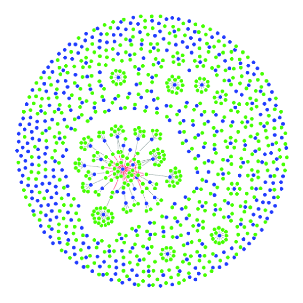
Figure 4: Network of the estimated regulatory relationships between the copy numbers of the 384 CNAIs and the expressions of the 654 breast cancer related genes. Each blue node stands for one CNAI, and each green node stands for one gene. Red edges represent inferred trans-regulations (43 in total). Grey edges represent cis-regulations.

We select tuning parameters $(\lambda_{1},\lambda_{2})$ in the remMap model through a 10-fold cross validation as described in Section 2.3. The optimal $(\lambda_{1},\lambda_{2}$) corresponding to the smallest CV score from a grid search is $(355.1,266.7)$. The resulting model contains $56$ trans-regulations in total. In order to further control false positive findings, we apply the cv.vote procedure with $V_{a}=5$, and filter away $13$ out of these $56$ trans-edges which have not been consistently selected across different CV folds. The remaining $43$ trans-edges correspond to three contiguous CNAIs on chromosome 17 and $31$ distinct (unlinked) RNAs. Figure 4 illustrates the topology of the estimated regulatory relationships. The detailed annotations of the three CNAIs and $31$ RNAs are provided in Table 3 and Table 4.

Table 3: Genome locations of the three CNAIs having (estimated) trans-regulations.

Index	Cytoband	Begin1	End 1	$\#$ of clones2	$\#$ of Trans-Reg3
1	17q12-17q12	34811630	34811630	1	12
2	17q12-17q12	34944071	35154416	9	30
3	17q21.1-17q21.2	35493689	35699243	7	1
1. Nucleotide position (bp).
2. Number of genes/clones on the array falling into the CNAI.
3. Number of unlinked genes whose expressions are estimated to be regulated by the CNAI.

Moreover, the Pearson-correlations between the DNA copy numbers of CNAIs and the expression levels of the regulated genes/clones (including both cis-regulation and trans-regulation) across the $172$ samples are reported in Table 4. As expected, all the cis-regulations have much higher correlations than the potential trans-regulations. In addition, none of the subtype indicator variables is selected into the final model, which implies that the detected associations between copy numbers of CNAIs and gene expressions are unlikely due to the stratification of the five tumor subtypes.

Table 4: RNAs¹ being influenced by the amplifications of the three CNAIs in Table 3.

Clone ID	Gene symbol	Cytoband	Correlation
753692	ABLIM1	10q25	0.199
896962	ACADS	12q22-qter	-0.22
753400	ACTL6A	3q26.33	0.155
472185	ADAMTS1	21q21.2	0.214
210687	AGTR1	3q21-q25	-0.182
856519	ALDH3A2	17p11.2	-0.244
270535	BM466581	19	0.03
238907	CABC1	1q42.13	-0.174
773301	CDH3	16q22.1	0.118
505576	CORIN	4p13-p12	0.196
223350	CP	3q23-q25	0.184
810463	DHRS7B	17p12	-0.151
50582	FLJ25076	5p15.31	0.086
669443	HSF2	6q22.31	0.207
743220	JMJD4	1q42.13	-0.19
43977	KIAA0182	16q24.1	0.259
810891	LAMA5	20q13.2-q13.3	0.269
247230	MARVELD2	5q13.2	-0.214
812088	NLN	5q12.3	0.093
257197	NRBF2	10q21.2	0.275
782449	PCBP2	12q13.12-q13.13	-0.079
796398	PEG3	19q13.4	0.169
293950	PIP5K1A	1q22-q24	-0.242
128302	PTMS	12p13	-0.248
146123	PTPRK	6q22.2-q22.3	0.218
811066	RNF41	12q13.2	-0.247
773344	SLC16A2	Xq13.2	0.24
1031045	SLC4A3	2q36	0.179
141972	STT3A	11q23.3	0.182
454083	TMPO	12q22	0.175
825451	USO1	4q21.1	0.204
68400	BM455010	17	0.748
756253,365147	ERBB2	17q11.2-q12—17q21.1	0.589
510318,236059	GRB7	17q12	0.675
245198	MED24	17q21.1	0.367
825577	STARD3	17q11-q12	0.664
7827562	TBPL1	6q22.1-q22.3	0.658
1. The first part of the table lists the inferred trans-regulated genes. The second
part of the table lists cis-regulated genes.
2. This cDNA sequence probe is annotated with TBPL1, but actually
maps to one of the 17q21.2 genes.

The three CNAIs being identified as trans-regulators sit closely on chromosome $17$, spanning from 34811630bp to 35699243bp and falling into cytoband 17q12-q21.2. This region (referred to as CNAI-17q12 hereafter) contains 24 known genes, including the famous breast cancer oncogene ERBB2, and the growth factor receptor-bound protein 7 (GRB7). The over expression of GRB7 plays pivotal roles in activating signal transduction and promoting tumor growth in breast cancer cells with chromosome 17q11-21 amplification Bai:2008. In this study, CNAI-17q12 is highly amplified (normalized $log_{2}$ ratio$>5$) in 33 ($19\%$) out of the $172$ tumor samples. Among the $654$ genes/clones considered in the above analysis, $8$ clones (corresponding to six genes including ERBB2, GRB7, and MED24) fall into this region. The expressions of these 8 clones are all up-regulated by the amplification of CNAI-17q12 (see Table 4 for more details), which is consistent with results reported in the literature Kao:2006. More importantly, as suggested by the result of the remMap model, the amplification of CNAI-17q12 also influences the expression levels of 31 unlinked genes/clones. This implies that CNAI-17q12 may harbor transcriptional factors whose activities closely relate to breast cancer. Indeed, there are 4 transcription factors (NEUROD2, IKZF3, THRA, NR1D1) and 2 transcriptional co-activators (MED1, MED24) in CNAI-17q12. It is possible that the amplification of CNAI-17q12 results in the over expression of one or more transcription factors/co-activators in this region, which then influence the expressions of the unlinked 31 genes/clones. In addition, some of the 31 genes/clones have been reported to have functions directly related to cancer and may serve as potential drug targets (see Appendix C.6 of the supplementary material for more details). In the end, we want to point out that, besides RNA interactions and subtype stratification, there could be other unaccounted confounding factors. Therefore, caution must be applied when one tries to interpret these results.

5 Discussion

In this paper, we propose the remMap method for fitting multivariate regression models under the large $P,Q$ setting. We focus on model selection, i.e., the identification of relevant predictors for each response variable. remMap is motivated by the rising needs to investigate the regulatory relationships between different biological molecules based on multiple types of high dimensional omics data. Such genetic regulatory networks are usually intrinsically sparse and harbor hub structures. Identifying the hub regulators (master regulators) is of particular interest, as they play crucial roles in shaping network functionality. To tackle these challenges, remMap utilizes a MAP penalty, which consists of an $\ell_{1}$ norm part for controlling the overall sparsity of the network, and an $\ell_{2}$ norm part for further imposing a row-sparsity of the coefficient matrix, which facilitates the detection of master predictors (regulators). This combined regularization takes into account both model interpretability and computational tractability. Since the MAP penalty is imposed on the coefficient matrix as a whole, it helps to borrow information across different regressions and thus incorporates the relationships among response variables into the model. As illustrated in Section 3, this type of “joint” modeling greatly improves model efficiency. Also, the combined $\ell_{1}$ and $\ell_{2}$ norm penalty further enhances the performance on both edge detection and master predictor identification.

We also propose a cv.vote procedure to make better use of the cross validation results. The idea is to treat the training data from each cross-validation fold as a “bootstrap” sample and identify the variables consistently selected in the majority of the cross-validation folds. As suggested by the simulation study, this procedure is very effective in decreasing the number of false positives while only slightly increases the number of false negatives. Moreover, cv.vote can be applied to a broad range of model selection problems when cross validation is employed.

In the real application, we apply the remMap method on a breast cancer data set. Our goal is to investigate the influences of DNA copy number alterations on RNA transcript levels based on $172$ breast cancer tumor samples. The resulting model suggests the existence of a trans-hub region on cytoband 17q12-q21, whose amplification influences RNA levels of $31$ unlinked genes. Cytoband 17q12-q21 is a well known hot region for breast cancer, which harbors the oncogene ERBB2. The above results suggest that this region may also harbor important transcriptional factors. While our findings are intriguing, clearly additional investigation is warranted. One way to verify the above conjecture is through a sequence analysis to search for common motifs in the upstream regions of the 31 RNA transcripts, which remains as our future work.

Besides the above application, the remMap model can be applied to investigate the regulatory relationships between other types of biological molecules. For example, it is of great interest to understand the influence of single nucleotide polymorphism (SNP) on RNA transcript levels, as well as the influence of RNA transcript levels on protein expression levels. Such investigation will improve our understanding of related biological systems as well as disease pathology. In addition, we can utilize the remMap idea to other models. For example, when selecting a group of variables in a multiple regression model, we can impose both the $\ell_{2}$ penalty (that is, the group lasso penalty), as well as an $\ell_{1}$ penalty to encourage within group sparsity. Similarly, the remMap idea can also be applied to vector autoregressive models and generalize linear models.

R package remMap is public available through CRAN ($http://cran.r-project.org/$).

(a) Impact of signal size $s$. $P=Q=600$, $N=200$; $\rho_{x}=0.4$; $\rho_{\varepsilon}=0$; the total number of trans-edges is $132$.

(b) Impact of predictor and response dimensionality $P$ $(Q=P)$. $N=200$; $s=0.25$; $\rho_{x}=0.4$; $\rho_{\varepsilon}=0$; the total number of trans-edges is $132$.

Figure 1: Impact of signal size and dimensionality. Heights of solid bars represent numbers of false positive detections of trans-edges (FP); heights of shaded bars represent numbers of false negative detections of trans-edges (FN). All bars are truncated at height=$132$.

(a) Impact of predictor correlation $\rho_{x}$. $P=Q=600$, $N=200$; $s=0.25$; $\rho_{\varepsilon}=0$; the total number of trans-edges is $132$.

(b) Impact of residual correlation $\rho_{\varepsilon}$. $P=Q=600$, $N=200$; $s=0.25$; $\rho_{x}=0.4$; the total number of trans-edges is $132$.

Figure 2: Impact of correlations. Heights of solid bars represent numbers of false positive detections of trans-edges (FP); heights of shaded bars represent numbers of false negative detections of trans-edges (FN). All bars are truncated at height=$132$.

Figure 3: (a) Direct interaction between CNAI A and the expression of gene B; (b) indirect interaction between CNAI A and the expression of Gene B through one intermediate gene.

Supplementary Material

Appendix A: Proof of Theorem 1

Define

$$L(\beta;Y,X)=\frac{1}{2}\sum_{q=1}^{Q}(y_{q}-x\beta_{q})^{2}+\lambda_{1}\sum_{q=1}^{Q}|\beta_{q}|+\lambda_{2}\sqrt{\sum_{q=1}^{Q}\beta_{q}^{2}}.$$

It is obvious that, in order to prove Theorem 1, we only need to show that, the solution of $\min_{\beta}L(\beta;Y,X)$, is given by (for $q=1,\cdots,Q$)

$$\widehat{\beta}_{q}=\left\{\begin{array}[]{ll}0,&\textrm{if}~{}||\widehat{\beta}^{\textrm{lasso}}||_{2}=0;\\ \widehat{\beta}^{\textrm{lasso}}_{q}\left(1-\frac{\lambda_{2}}{||\widehat{\beta}^{\textrm{lasso}}||_{2}x^{2}}\right)_{+},&\textrm{otherwise},\\ \end{array}\right.$$

where

$$\widehat{\beta}^{\textrm{lasso}}_{q}=\left(1-\frac{\lambda_{1}}{|xy_{q}|}\right)_{+}\frac{xy_{q}}{x^{2}}.$$ (S-2)

In the following, for function $L$, view $\{\beta_{q^{\prime}}:q^{\prime}\neq q\}$ as fixed. With a slight abuse of notation, write $L=L(\beta_{q})$. Then when $\beta_{q}\geq 0$, we have

$$\frac{dL}{d\beta_{q}}=-xy_{q}+(x^{2}+\frac{\lambda_{2}}{||\beta||_{2}})\beta_{q}+\lambda_{1}.$$

Thus, $\frac{dL}{d\beta_{q}}>0$ if and only if $\beta_{q}>\tilde{\beta_{q}}^{+}$, where

$$\tilde{\beta_{q}}^{+}:=\frac{xy_{q}}{x^{2}+\frac{\lambda_{2}}{||\beta||_{2}}}(1-\frac{\lambda_{1}}{xy_{q}}).$$

Denote the minima of $L(\beta_{q})|_{\beta_{q}\geq 0}$ by $\beta_{q,\textrm{min}}^{+}$. Then, when $\tilde{\beta_{q}}^{+}>0$, $\beta_{q,\textrm{min}}^{+}=\tilde{\beta_{q}}^{+}$. On the other hand, when $\tilde{\beta_{q}}^{+}\leq 0$, $\beta_{q,\textrm{min}}^{+}=0$. Note that $\tilde{\beta_{q}}^{+}>0$ if and only if $xy_{q}(1-\frac{\lambda_{1}}{xy_{q}})>0$. Thus we have

$$\beta_{q,\textrm{min}}^{+}=\left\{\begin{array}[]{ll}\tilde{\beta}_{q}^{+},&\textrm{if}~{}xy_{q}(1-\frac{\lambda_{1}}{xy_{q}})>0;\\ 0,&\textrm{if}~{}xy_{q}(1-\frac{\lambda_{1}}{xy_{q}})\leq 0.\\ \end{array}\right.$$

Similarly, denote the minima of $L(\beta_{q})|_{\beta_{q}\leq 0}$ by $\beta_{q,\textrm{min}}^{-}$, and define

$$\tilde{\beta_{q}}^{-}:=\frac{xy_{q}}{x^{2}+\frac{\lambda_{2}}{||\beta||_{2}}}(1+\frac{\lambda_{1}}{xy_{q}}).$$

Then we have

$$\beta_{q,\textrm{min}}^{-}=\left\{\begin{array}[]{ll}\tilde{\beta}_{q}^{-},&\textrm{if}~{}xy_{q}(1+\frac{\lambda_{1}}{xy_{q}})<0;\\ 0,&\textrm{if}~{}xy_{q}(1+\frac{\lambda_{1}}{xy_{q}})\geq 0.\\ \end{array}\right.$$

Denote the minima of $L(\beta_{q})$ as $\widehat{\beta}_{q}$ (with a slight abuse of notation). From the above, it is obvious that, if $xy_{q}>0$, then $\widehat{\beta}_{q}\geq 0$. Thus $\widehat{\beta}_{q}=\max(\tilde{\beta}_{q}^{+},0)=\frac{xy_{q}}{x^{2}+\frac{\lambda_{2}}{||\beta||_{2}}}(1-\frac{\lambda_{1}}{xy_{q}})_{+}=\frac{xy_{q}}{x^{2}+\frac{\lambda_{2}}{||\beta||_{2}}}(1-\frac{\lambda_{1}}{|xy_{q}|})_{+}$. Similarly, if $xy_{q}\leq 0$, then $\widehat{\beta}_{q}\leq 0$, and it has the same expression as above. Denote the minima of $L(\beta)|_{||\beta||_{2}>0}$ (now viewed as a function of $(\beta_{1},\cdots,\beta_{Q})$) as $\widehat{\beta}_{\textrm{min}}=(\widehat{\beta}_{1,\textrm{min}},\cdots,\widehat{\beta}_{Q,\textrm{min}})$. We have shown above that, if such a minima exists, it satisfies (for $q=1,\cdots,Q$)

$$\widehat{\beta}_{q,\textrm{min}}=\frac{xy_{q}}{x^{2}+\frac{\lambda_{2}}{||\widehat{\beta}_{\textrm{min}}||_{2}}}\left(1-\frac{\lambda_{1}}{|xy_{q}|}\right)_{+}=\widehat{\beta}_{q}^{\textrm{lasso}}\frac{x^{2}}{x^{2}+\frac{\lambda_{2}}{||\widehat{\beta}_{\textrm{min}}||_{2}}},$$ (S-5)

where $\widehat{\beta}_{q}^{\textrm{lasso}}$ is defined by equation (S-2). Thus

$$||\widehat{\beta}_{\textrm{min}}||_{2}=||\widehat{\beta}^{\textrm{lasso}}||_{2}\frac{x^{2}}{x^{2}+\frac{\lambda_{2}}{||\widehat{\beta}_{\textrm{min}}||_{2}}}.$$

By solving the above equation, we obtain

$$||\widehat{\beta}_{\textrm{min}}||_{2}=||\widehat{\beta}^{\textrm{lasso}}||_{2}-\frac{\lambda_{2}}{x^{2}}.$$

By plugging the expression on the right hand side into (S-5), we achieve

$$\widehat{\beta}_{q,\textrm{min}}=\widehat{\beta}_{q}^{\textrm{lasso}}\left(1-\frac{\lambda_{2}}{||\widehat{\beta}^{\textrm{lasso}}||_{2}x^{2}}\right).$$

Denote the minima of $L(\beta)$ by $\widehat{\beta}=(\widehat{\beta}_{1},\cdots,\widehat{\beta}_{Q})$. From the above, we also know that if $||\widehat{\beta}^{\textrm{lasso}}||_{2}-\frac{\lambda_{2}}{x^{2}}>0$, $L(\beta)$ achieves its minimum on $||\beta||_{2}>0$, which is $\widehat{\beta}=\widehat{\beta}_{\textrm{min}}$. Otherwise, $L(\beta)$ achieves its minimum at zero. Since $||\widehat{\beta}^{\textrm{lasso}}||_{2}-\frac{\lambda_{2}}{x^{2}}>0$ if and only if $1-\frac{\lambda_{2}}{||\widehat{\beta}^{\textrm{lasso}}||_{2}x^{2}}>0$, we have proved the theorem.

Appendix B: BIC criterion for tuning

In this section, we describe the BIC criterion for selecting $(\lambda_{1},\lambda_{2})$. We also derive an unbiased estimator of the degrees of freedom of the remMap estimator under orthogonal design.

In model (1), by assuming $\epsilon_{q}\sim{\rm Normal}(0,\sigma^{2}_{q,\epsilon})$, the BIC criterion for the $q^{th}$ regression can be defined as

$${\rm BIC}_{q}(\widehat{\beta}_{1q},\cdots,\widehat{\beta}_{Pq};{\rm df}_{q})=N\times\log({\rm RSS}_{q})+\log N\times{\rm df}_{q},$$ (S-6)

where ${\rm RSS}_{q}:=\sum_{n=1}^{N}(y^{n}_{q}-\widehat{y}^{n}_{q})^{2}$ with $\widehat{y}^{n}_{q}=\sum_{p=1}^{P}x^{n}_{p}\widehat{\beta}_{pq}$; and ${\rm df}_{q}$ is the degrees of freedom which is defined as

$${\rm df}_{q}={\rm df}_{q}(\widehat{\beta}_{1q},\cdots,\widehat{\beta}_{Pq}):=\sum_{n=1}^{N}{\rm Cov}(\widehat{y}^{n}_{q},y^{n}_{q})/\sigma^{2}_{q,\epsilon},$$ (S-7)

where $\sigma^{2}_{q,\epsilon}$ is the variance of $\epsilon_{q}$.

For a given pair of $(\lambda_{1},\lambda_{2})$, We then define the (overall) BIC criterion at $(\lambda_{1},\lambda_{2})$:

$${\rm BIC}(\lambda_{1},\lambda_{2})=N\times\sum_{q=1}^{Q}\log({\rm RSS}_{q}(\lambda_{1},\lambda_{2}))+\log N\times\sum_{q=1}^{Q}{\rm df}_{q}(\lambda_{1},\lambda_{2}).$$ (S-8)

lars derive an explicit formula for the degrees of freedom of lars under orthogonal design. Similar strategy are also used by YuanLin:2006 among others. In the following theorem, we follow the same idea and derive an unbiased estimator of $df_{q}$ for remMap when the columns of $\mathbf{X}$ are orthogonal to each other.

Theorem 2

Suppose $X_{p}^{T}X_{p^{\prime}}=0$ for all $1\leq p\not=p^{\prime}\leq P$. Then for given $(\lambda_{1},\lambda_{2})$,

$$\widehat{df}_{q}(\lambda_{1},\lambda_{2}) := \sum_{p=1}^{P}c_{pq}\times\mathbb{I}\left(||\widehat{B}_{p}^{\rm lasso}||_{2,C}>\frac{\lambda_{2}}{||X_{p}||^{2}_{2}}\right)\times\mathbb{I}\left(|\widehat{\beta}_{pq}^{\rm ols}|>\frac{\lambda_{1}}{||X_{p}||^{2}_{2}}\right)$$ (S-9)

$$\times \left(1-\frac{\lambda_{2}}{||X_{p}||^{2}_{2}}\frac{||\widehat{B}_{p}^{\rm lasso}||_{2,C}^{2}-(\widehat{\beta}^{\rm lasso}_{pq})^{2}}{||\widehat{B}_{p}^{\rm lasso}||_{2,C}^{3}}\right)+\sum_{p=1}^{P}(1-c_{p,q})$$

is an unbiased estimator of the degrees of freedom ${\rm df}_{q}(\lambda_{1},\lambda_{2})$ (defined in equation (S-7)) of the remMap estimator $\widehat{\mathbf{B}}=\widehat{\mathbf{B}}(\lambda_{1},\lambda_{2})=(\widehat{\beta}_{pq}(\lambda_{1},\lambda_{2}))$. Here, under the orthogonal design, $\widehat{\beta}_{pq},\widehat{\beta}_{pq}^{\rm lasso}$ are given by Theorem 1 with $\widetilde{Y}_{q}=Y_{q}$ ($q=1,\cdots,Q$), and $\widehat{\beta}^{\rm ols}_{pq}:=\frac{X_{p}^{T}Y_{q}}{||X_{p}||^{2}_{2}}$.

Before proving Theorem 2, we first explain definition (S-7) – the degrees of freedom. Consider the $q^{th}$ regression in model (1). Suppose that $\{\widehat{y}^{n}_{q}\}_{n=1}^{N}$ are the fitted values by a certain fitting procedure based on the current observations $\{y^{n}_{q}:n=1,\cdots,N;q=1,\cdots,Q\}$. Let $\mu^{n}_{q}:=\sum_{p=1}^{P}x^{n}_{p}\beta_{pq}$. Then for a fixed design matrix $X=(x^{n}_{p})$, the expected re-scaled prediction error of $\{\widehat{y}^{n}_{q}\}_{n=1}^{N}$ in predicting a future set of new observations $\{\widetilde{y}^{n}_{q}\}_{n=1}^{N}$ from the $q^{th}$ regression of model (1) is:

$${\rm PE}_{q}=\sum_{n=1}^{N}E((\widehat{y}^{n}_{q}-\widetilde{y}^{n}_{q})^{2})/\sigma^{2}_{q,\epsilon}=\sum_{n=1}^{N}E((\widehat{y}^{n}_{q}-\mu^{n}_{q})^{2})/\sigma^{2}_{q,\epsilon}+N.$$

Note that

$$(\widehat{y}^{n}_{q}-y^{n}_{q})^{2}=(\widehat{y}^{n}_{q}-\mu^{n}_{q})^{2}+(y^{n}_{q}-\mu^{n}_{q})^{2}-2(\widehat{y}^{n}_{q}-\mu^{n}_{q})(y^{n}_{q}-\mu^{n}_{q}).$$

Therefore,

$${\rm PE}_{q}=\sum_{n=1}^{N}E((\widehat{y}^{n}_{q}-y^{n}_{q})^{2})/\sigma^{2}_{q,\epsilon}+2\sum_{n=1}^{N}{\rm Cov}(\widehat{y}^{n}_{q},y^{n}_{q})/\sigma^{2}_{q,\epsilon}.$$

Denote $RSS_{q}=\sum_{n=1}^{N}(\widehat{y}^{n}_{q}-y^{n}_{q})^{2}$. Then an un-biased estimator of ${\rm PE}_{q}$ is

$$RSS_{q}/\sigma^{2}_{q,\epsilon}+2\sum_{n=1}^{N}{\rm Cov}(\widehat{y}^{n}_{q},y^{n}_{q})/\sigma^{2}_{q,\epsilon}.$$

Therefore, a natural definition of the degrees of freedom for the procedure resulting the fitted values $\{\widehat{y}^{n}_{q}\}_{n=1}^{N}$ is as given in equation (S-7). Note that, this is the definition used in Mallow’s $C_{p}$ criterion.

Proof of Theorem 2: By applying Stein’s identity to the Normal distribution, we have: if $Z\sim N(\mu,\sigma^{2})$, and a function $g$ such that $E(|g^{\prime}(Z)|)<\infty$, then

$${\rm Cov}(g(Z),Z)/\sigma^{2}=E(g^{\prime}(Z)).$$

Therefore, under the normality assumption on the residuals $\{\epsilon_{q}\}_{q=1}^{Q}$ in model (1), definition (S-7) becomes

$$df_{q}=\sum_{n=1}^{N}E\left(\frac{\partial\widehat{y}^{n}_{q}}{\partial y^{n}_{q}}\right),\quad q=1,\cdots,Q.$$

Thus an obvious unbiased estimator of $df_{q}$ is $\widehat{df}_{q}=\sum_{n=1}^{N}\frac{\partial\widehat{y}^{n}_{q}}{\partial y^{n}_{q}}$. In the following, we derive $\widehat{df}_{q}$ for the proposed remMap estimator under the orthogonal design. Let $\widehat{\beta}_{q}=(\widehat{\beta}_{1q},\cdots,\widehat{\beta}_{Pq})$ be a one by $P$ row vector; let $\mathbf{X}=(x^{n}_{p})$ be the $N$ by $P$ design matrix which is orthonormal; let $Y_{q}=(y^{1}_{1},\cdots,y^{N}_{q})^{T}$ and $\widehat{Y}_{q}=(\widehat{y}^{1}_{q},\cdots,\widehat{y}^{N}_{q})^{T}=\mathbf{X}\widehat{\beta}_{q}$ be $N$ by one column vectors. Then

$$\widehat{df}_{q}={\rm tr}\left(\frac{\partial\widehat{Y}_{q}}{\partial Y_{q}}\right)={\rm tr}\left(\mathbf{X}\frac{\partial\widehat{\beta}_{q}}{\partial Y_{q}}\right)={\rm tr}\left(\mathbf{X}\frac{\partial\widehat{\beta}_{q}}{\partial\widehat{\beta}_{q,\textrm{ols}}}\frac{\partial\widehat{\beta}_{q,\textrm{ols}}}{\partial Y_{q}}\right),$$

where $\widehat{\beta}_{q,\textrm{ols}}=(\widehat{\beta}^{\textrm{ols}}_{1q},\cdots,\widehat{\beta}^{\textrm{ols}}_{Pq})^{T}$ and the last equality is due to the chain rule. Since under the orthogonal design, $\widehat{\beta}^{\textrm{ols}}_{pq}=X_{p}^{T}Y_{q}/||X_{p}||^{2}_{2}$, where $X_{p}=(x^{1}_{p},\cdots,x^{N}_{p})^{T}$, thus $\frac{\partial\widehat{\beta}_{q,\textrm{ols}}}{\partial Y_{q}}=\mathbf{D}\mathbf{X}^{T},$ where $\mathbf{D}$ is a $P$ by $P$ diagonal matrix with the $p^{th}$ diagonal entry being $1/||X_{p}||^{2}_{2}$. Therefore

$$\widehat{df}_{q}={\rm tr}\left(\mathbf{X}\frac{\partial\widehat{\beta}_{q}}{\partial\widehat{\beta}_{q,\textrm{ols}}}\mathbf{D}\mathbf{X}^{T}\right)={\rm tr}\left(\mathbf{D}\mathbf{X}^{T}\mathbf{X}\frac{\partial\widehat{\beta}_{q}}{\partial\widehat{\beta}_{q,\textrm{ols}}}\right)={\rm tr}\left(\frac{\partial\widehat{\beta}_{q}}{\partial\widehat{\beta}_{q,\textrm{ols}}}\right)=\sum_{p=1}^{P}\frac{\partial\widehat{\beta}_{pq}}{\partial\widehat{\beta}^{\textrm{ols}}_{pq}},$$

where the second to last equality is by $\mathbf{X}^{T}\mathbf{X}=\mathbf{D}^{-1}$ which is due to the orthogonality of $\mathbf{X}$. By the chain rule

$$\frac{\partial\widehat{\beta}_{pq}}{\partial\widehat{\beta}^{\textrm{ols}}_{pq}}=\frac{\partial\widehat{\beta}_{pq}}{\partial\widehat{\beta}^{\textrm{lasso}}_{pq}}\frac{\partial\widehat{\beta}^{\textrm{lasso}}_{pq}}{\partial\widehat{\beta}^{\textrm{ols}}_{pq}}.$$

By Theorem 1, under the orthogonal design,

$$\frac{\partial\widehat{\beta}_{pq}}{\partial\widehat{\beta}^{\textrm{lasso}}_{pq}}=\mathbb{I}\left(||\widehat{B}_{p}^{\textrm{lasso}}||_{2,C}>\frac{\lambda_{2}}{||X_{p}||_{2}^{2}}\right)\times\left[1-\frac{\lambda_{2}}{||X_{p}||_{2}^{2}}\frac{||\widehat{B}_{p}^{\textrm{lasso}}||^{2}_{2,C}-(\widehat{\beta}^{\textrm{lasso}}_{pq})^{2}}{||\widehat{B}_{p}^{\textrm{lasso}}||^{3}_{2,C}}\right],$$

and

$$\frac{\partial\widehat{\beta}^{\textrm{lasso}}_{pq}}{\partial\widehat{\beta}^{\textrm{ols}}_{pq}}=\left\{\begin{array}[]{ll}1,&\textrm{if}~{}c_{p,q}=0;\\ \mathbb{I}\left(|\widehat{\beta}^{\textrm{ols}}_{pq}|>\frac{\lambda_{1}}{||X_{p}||^{2}_{2}}\right),&\textrm{if}~{}c_{p,q}=1.\end{array}\right.$$

Note that when $c_{p,q}=0$, $\widehat{\beta}_{pq}=\widehat{\beta}^{\textrm{ols}}_{pq}$, thus $\frac{\partial\widehat{\beta}_{pq}}{\partial\widehat{\beta}^{\textrm{ols}}_{pq}}=1$. It is then easy to show that $\widehat{df}_{q}$ is as given in equation (S-9).

Note that, when the $\ell_{2}$ penalty parameter $\lambda_{2}$ is 0, the model becomes $q$ separate lasso regressions with the same penalty parameter $\lambda_{1}$ and the degrees of freedom estimation in equation (S-9) is simply the total number of non-zero coefficients in the model (under orthogonal design). When $\lambda_{2}$ is nonzero, the degrees of freedom of remMap estimator should be smaller than the number of non-zero coefficients due to the additional shrinkage induced by the $\ell_{2}$ norm part of the MAP penalty (equation (3)). This is reflected by equation (S-9).

Appendix C: Data Preprocessing

C.1 Preprocessing for array CGH data

Each array output ($log_{2}$ ratios) is first standardized to have median$=0$ and smoothed by cghFLasso cghFLasso2008 for defining gained/lost regions on the genome. The noise level of each array is then calculated based on the measurements from the estimated normal regions (i.e., regions with estimated copy numbers equal to 2). After that, each smoothed array is normalized according to its own noise level.

We define copy number alteration intervals (CNAIs) by using the Fixed-Order Clustering (FOC) method  Wang:thesis. FOC first builds a hierarchical clustering tree along the genome based on all arrays, and then cuts the tree at an appropriate height such that genes with similar copy numbers fall into the same CNAI. FOC is a generalization of the CLAC (CLuster Along Chromosome) method proposed by CLAC:2005. It differs in two ways from the standard agglomerative clustering. First, the order of the leaves in the tree is fixed, which represents the genome order of the genes/clones in the array. So, only adjacent clusters are joined together when the tree is generated by a bottom-up approach. Second, the similarity between two clusters no longer refers to the spatial distance but to the similarity of the array measurements ($log_{2}$ ratio) between the two clusters. By using FOC, the whole genome is divided into $384$ non-overlapping CNAIs based on all $172$ CGH arrays. This is illustrated in Figure S-1. In addition, the heatmap of the (sample) correlations of the CNAIs is given in Figure S-2.

C.2 Selection of breast cancer related genes

We combine seven published breast cancer gene lists: the intrinsic gene set Sorlie:2003, the Amsterdam 70 gene vandeVijver:2002, the wound response gene set  Chang:2004, the 76 genes for the metastasis signature Wang:2005, the gene list for calculating the recurrence score Paik:2004, the gene list of the Genomic Grade Index (GGI) Sotiriou:2006, and the PTEN gene set Saal:2007. Among this union set of breast cancer related genes, $967$ overlap with the genes in the current expression data set. We further filter away genes with missing measurements in more than $20\%$ of the samples, and $654$ genes are left. Among these $654$ selected genes, $449$ are from the intrinsic gene set Sorlie:2003, which are used to derive breast cancer subtype labels in Appendix C.4.

C.3 Interactions among RNA expressions

We apply the space (Sparse PArtial Correlation Estimation) method  space:2008 to infer the interactions among RNA levels through identifying non-zero partial correlations. space assumes the overall sparsity of the partial correlation matrix and employs sparse regression techniques for model fitting. As indicated by many experiments that genetic-regulatory networks have a power-law type degree distribution with a power parameter between 2 and 3 Newman:2003, the tuning parameter in space is chosen such that the resulting network has an estimated power parameter around $2$ (see Figure S-3(b) for the corresponding degree distribution). The resulting (concentration) network has $664$ edges in total, whose topology is illustrated in Figure S-3(a). In this network, there are 7 nodes having at least 10 edges. These hub genes include PLK1, PTTG1, AURKA, ESR1, and GATA3. PLK1 has important functions in maintaining genome stability via its role in mitosis. Its over expression is associated with preinvasive in situ carcinomas of the breast Rizki:2007. PTTG1 is observed to be a proliferation marker in invasive ductal breast carcinomas Talvinen:2008. AURKA encodes a cell cycle-regulated kinase and is a potential metastasis promoting gene for breast cancer Thomassen:2008. ESR1 encodes an estrogen receptor, and is a well known key player in breast cancer. Moreover, it had been reported that GATA3 expression has a strong association with estrogen receptor in breast cancer Voduc:2008. Detailed annotation of these and other hub genes are listed in Table S-1. We refer to this network as Exp.Net.664, and use it to account for RNA interactions when investigating the regulations between CNAIs and RNA levels.

Table S-1: Annotations for hub genes (degrees greater than 10) in the inferred RNA interaction network Exp.Net.664.

CloneID	Gene Name	Symbol	ID	Cytoband
744047	Polo-like kinase 1 (Drosophila)	PLK1	5347	16p12.1
781089	Pituitary tumor-transforming 1	PTTG1	9232	5q35.1
129865	Aurora kinase A	AURKA	6790	20q13.2-q13.3
214068	GATA binding protein 3	GATA3	2625	10p15
950690	Cyclin A2	CCNA2	890	4q25-q31
120881	RAB31, member RAS oncogene family	RAB31	11031	18p11.3
725321	Estrogen receptor 1	ESR1	2099	6q25.1

C.4 Breast Cancer Subtypes

Population stratification due to distinct subtypes could confound our detection of associations between CNAIs and gene expressions. For example, if the copy number of CNAI A and expression level of gene B are both higher in one subtype than in the other subtypes, we could observe a strong correlation between CNAI A and gene expression B across the whole population, even when the correlation within each subtype is rather weak. To account for this potential confounding factor, we introduce a set of subtype indicator variables, which is used as additional predictors in the remMap model. Specifically, we derive subtype labels based on expression patterns by following the work of Sorlie:2003. We first normalize the expression levels of each intrinsic gene ($449$ in total) across the $172$ samples to have mean zero and MAD one. Then we use kmeans clustering to divide the patients into five distinct groups, which correspond to the five subtypes suggested by Sorlie:2003 — Luminal Subtype A, Luminal Subtype B, ERBB2-overexpressing Subtype, Basal Subtype and Normal Breast-like Subtype. Figure S-4 illustrates the expression patterns of these five subtypes across the $172$ samples. We then define five dummy variables to represent the subtype information for each tumor sample, and include them as predictors when fitting the remMap model.

C.5 Comments on the results of the remMap analysis.

remMap analysis suggests that the amplification of a trans-hub region on chromosome 17 influences the RNA expression levels of $31$ distinct (unlinked) genes. Some of the 31 genes/clones have been reported to have functions directly related to cancer and may serve as potential drug targets. For example, AGTR1 is a receptor whose genetic polymorphisms have been reported to associate with breast cancer risk and is possibly druggable Koh:2005. CDH3 encodes a cell-cell adhesion glycoprotein and is deemed as a candidate of tumor suppressor gene, as disturbance of intracellular adhesion is important for invasion and metastasis of tumor cells Kremmidiotis:1998. PEG3 is a mediator between p53 and Bax in DNA damage-induced neuronal death  Johnson:2002 and may function as a tumor suppressor gene Dowdy:2005. In a word, these 31 genes may play functional roles in the pathogenesis of breast cancer and may serve as additional targets for therapy.

Figure S-1: Hierarchical tree constructed by FOC. Each leaf represents one gene/clone on the array. The order of the leaves represents the order of genes on the genome. The 23 Chromosomes are illustrated with different colors. Cutting the tree at 0.04 (horizonal red line) separates the genome into 384 intervals. This cutoff point is chosen such that no interval contains genes from different chromosomes.

Figure S-2: Heatmaps of the sample correlations among predictors. Top panel: simulated data; Bottom panel: real data

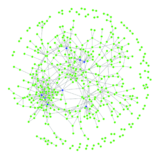
(a) Exp.Net.664: Inferred network for the 654 breast cancer related genes (based on their expression levels) by space. Nodes with degrees greater than ten are drawn in blue.

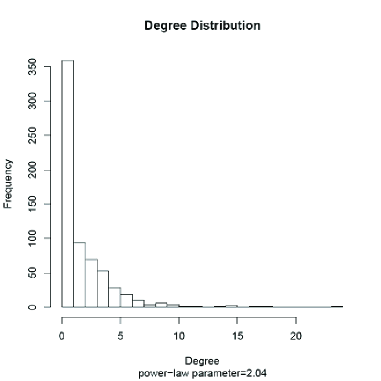
(b) Degree distribution of network Exp.Net.664.

Figure S-3: Inferred RNA interaction network.

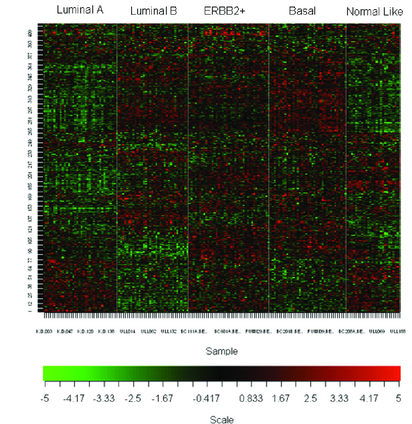
Figure S-4: Heatmap showing the expressions of the 449 intrinsic genes in the 172 breast cancer tumor samples. Each column represents one sample and each row represents one gene. The 172 samples are divided into 5 clusters (subtypes). From the left to the right, the 5 subtypes are: Luminal Subtype A, Luminal Subtype B, ERBB2-overexpressing subtype, Basal Subtype and Normal Breast-like Subtype.

References

- [\citeauthoryearAlbertson et al.Albertson et al.2003] Albertson, D. G., C. Collins, F. McCormick, and J. W. Gray, (2003), “Chromosome aberrations in solid tumors,” Nature Genetics, 34.
- [\citeauthoryearAntoniadis and FanAntoniadis and Fan2001] Antoniadis, A., and Fan, J., (2001), “Regularization of wavelet approximations,” Journal of the American Statistical Association, 96, 939–967.
- [\citeauthoryearBai and LouhBai and Louh2008] Bai T, Luoh SW., (2008) “GRB-7 facilitates HER-2/Neu-mediated signal transduction and tumor formation,” Carcinogenesis, 29(3), 473-9.
- [\citeauthoryearBakinBakin1999] Bakin, S., (1999), “Adaptive regression and model selection in data mining problems,” PhD Thesis , Australian National University, Canberra.
- [\citeauthoryearBedrick et al.Bedrick et al.1994] Bedrick, E. and Tsai, C.,(1994), “Model selection for multivariate regression in small samples,” Biometrics, 50, 226 C231.
- [\citeauthoryearBergamaschi et al.Bergamaschi et al.2006] Bergamaschi, A., Kim, Y. H., Wang, P., Sorlie, T., Hernandez-Boussard, T., Lonning, P. E., Tibshirani, R., Borresen-Dale, A. L., and Pollack, J. R., (2006), “Distinct patterns of DNA copy number alteration are associated with different clinicopathological features and gene-expression subtypes of breast cancer,” Genes Chromosomes Cancer, 45, 1033-1040.
- [\citeauthoryearBergamaschi et al.Bergamaschi et al.2008] Bergamaschi, A., Kim, Y.H., Kwei, K.A., Choi, Y.L., Bocanegra, M., Langerod, A., Han, W., Noh, D.Y., Huntsman, D.G., Jeffrey, S.S., Borresen-Dale, A. L., and Pollack, J.R., (2008), “CAMK1D amplification implicated in epithelial-mesenchymal transition in basal-like breast cancer,” Mol Oncol, In Press.
- [\citeauthoryearBreiman et al.Breiman et al.1997] Breiman, L. and Friedman, J. H., (1997), “Predicting multivariate responses in multiple linear regression (with discussion),” J. R. Statist. Soc. B, 59, 3-54.
- [\citeauthoryearBrown et al.Brown et al.1999] Brown, P., Fearn, T. and Vannucci, M., (1999), “The choice of variables in multivariate regression: a non-conjugate Bayesian decision theory approach,” Biometrika, 86, 635 C648.
- [\citeauthoryearBrown et al.Brown et al.1998] Brown, P., Vannucci, M. and Fearn, T., (1998), “Multivariate Bayesian variable selection and prediction,” J. R. Statist. Soc. B, 60, 627 C641.
- [\citeauthoryearBrown et al.Brown et al.2002] Brown, P., Vannucci, M. and Fearn, T.,(2002), “Bayes model averaging with selection of regressors,” J. R. Statist. Soc. B, 64, 519 C536.
- [\citeauthoryearChang et al.Chang et al.2004] Chang HY, Sneddon JB, Alizadeh AA, Sood R, West RB, et al., (2004), “Gene expression signature of fibroblast serum response predicts human cancer progression: Similarities between tumors and wounds,” PLoS Biol, 2(2).
- [\citeauthoryearEfron, Hastie, Johnstone, and TibshiraniEfron et al.2004] Efron, B., Hastie, T., Johnstone, I., and Tibshirani, R. (2004), “Least Angle Regression,” Annals of Statistics, 32, 407–499.
- [\citeauthoryearFrank et al.Frank et al.1993] Frank, I. and Friedman, J.,(1993), “A statistical view of some chemometrics regression tools (with discussion),” Technometrics, 35, 109 C148.
- [\citeauthoryearFuFu1998] Fu, W., (1998), “Penalized regressions: the bridge vs the lasso,” Journal of Computational and Graphical Statistics, 7(3):417-433.
- [\citeauthoryearFriedman et al.Friedman et al.2008] Friedman, J., Hastie, T. and Tibshirani, R.,(2008), “Regularized Paths for Generalized Linear Models via Coordinate Descent,” Techniqual Report, Department of Statistics, Stanford University.
- [\citeauthoryearFriedman et al.Friedman et al.2007] Friedman, J., Hastie, T. and Tibshirani, R.,(2007), “Pathwise coordinate optimization,” The Annals of Applied Statistics., 1(2), 302-332 .
- [\citeauthoryearFujikoshi et al.Fujikoshi et al.1997] Fujikoshi,Y. and Satoh, K., (1997), “Modified AIC and Cp in multivariate linear regression,” Biometrika, 84, 707 C716.
- [\citeauthoryearGardner et al.Gardner et al.2003] Gardner, T. S., D. DI Bernardo, D. Lorenz, and J. J. Collins, (2003) “Inferring genetic networks and identifying compound mode of action via expression profiling,” Science, 301
- [\citeauthoryearHyman et al.Hyman et al.2002] Hyman, E., P. Kauraniemi, S. Hautaniemi, M. Wolf, S. Mousses, E. Rozenblum, M. Ringner, G. Sauter, O. Monni, A. Elkahloun, O.-P. Kallioniemi, and A. Kallioniemi, (2002), “Impact of dna amplification on gene expression patterns in breast cancer,” Cancer Res, 62.
- [\citeauthoryearIzenmanIzenman1975] Izenman, A., (1975), “Reduced-rank regression for the multivariate linear model,” J. Multiv. Anal., 5, 248 C264.
- [\citeauthoryearJeong et al.Jeong et al.2001] Jeong, H., S. P. Mason, A. L. Barabasi, and Z. N. Oltvai, (2001), “Lethality and centrality in protein networks,” Nature, (411)
- [\citeauthoryearKapp et al.Kapp et al.2006] Kapp, A. V., Jeffrey, S. S., Langerod, A., Borresen-Dale, A. L., Han, W., Noh, D. Y., Bukholm, I. R., Nicolau, M., Brown, P. O. and Tibshirani, R., (2006), “Discovery and validation of breast cancer subtypes,” BMC Genomics, 7, 231.
- [\citeauthoryearKao and PollackKao and Pollack2006] Kao J, Pollack JR., (2006), “RNA interference-based functional dissection of the 17q12 amplicon in breast cancer reveals contribution of coamplified genes,” Genes Chromosomes Cancer, 45(8), 761-9.
- [\citeauthoryearKim et al.Kim et al.2008] Kim, S., Sohn, K.-A., Xing E. P., (2008) “A multivariate regression approach to association analysis of quantitative trait network” http://arxiv.org/abs/0811.2026.
- [\citeauthoryearLangerod et al.Langerod et al.2007] Langerod, A., Zhao, H., Borgan, O., Nesland, J. M., Bukholm, I. R., Ikdahl, T., Karesen, R., Borresen-Dale, A. L., Jeffrey, S. S., (2007), “TP53 mutation status and gene expression profiles are powerful prognostic markers of breast cancer,” Breast Cancer Res, 9, R30.
- [\citeauthoryearLutz and BühlmannLutz and Bühlmann2006] Lutz, R. and Bühlmann, P., (2006), “Boosting for high-multivariate responses in high-dimensional linear regression,” Statist. Sin., 16, 471 C494.
- [\citeauthoryearObozinskiy et al.Obozinskiy et al.2008] Obozinskiy, G., Wainwrighty, M.J., Jordany, M. I., (2008) “Union support recovery in high-dimensional multivariate regression,” http://arxiv.org/abs/0808.0711.
- [\citeauthoryearPaik et al.Paik et al.2004] Paik S, Shak S, Tang G, Kim C, Baker J, et al., (2004), “A multigene assay to predict recurrence of tamoxifen-treated, node-negative breast cancer,” N Engl J Med, 351(27), 2817-2826.
- [\citeauthoryearPeng et al.Peng et al.2008] Peng, J., P. Wang, N. Zhou, J. Zhu, (2008), “Partial Correlation Estimation by Joint Sparse Regression Models,” JASA, to appear.
- [\citeauthoryearPollack et al.Pollack et al.2002] Pollack, J., T. Srlie, C. Perou, C. Rees, S. Jeffrey, P. Lonning, R. Tibshirani, D. Botstein, A. Brresen-Dale, and Brown,P., (2002), “Microarray analysis reveals a major direct role of dna copy number alteration in the transcriptional program of human breast tumors,” Proc Natl Acad Sci, 99(20).
- [\citeauthoryearReinsel and VeluReinsel and Velu1998] Reinsel, G. and Velu, R., (1998), “Multivariate Reduced-rank Regression: Theory and Applications,” New York, Springer.
- [\citeauthoryearSaal et al.Saal et al.2007] Saal LH, Johansson P, Holm K, Gruvberger-Saal SK, She QB, et al., (2007), “Poor prognosis in carcinoma is associated with a gene expression signature of aberrant PTEN tumor suppressor pathway activity,” Proc Natl Acad Sci U S A, 104(18), 7564-7569.
- [\citeauthoryearSorlie et al.Sorlie et al.2001] Sorlie, T., Perou, C. M., Tibshirani, R., Aas, T., Geisler, S., Johnsen, H., Hastie, T., Eisen, M. B., van de Rijn, M., Jeffrey, S. S., Thorsen, T., Quist, H., Matese,J. C., Brown,P. O., Botstein, D., L nning P. E., and B rresen-Dale, A.L., (2001), “Gene expression patterns of breast carcinomas distinguish tumor subclasses with clinical implications,” Proc Natl Acad Sci U S A, 98, 10869-10874.
- [\citeauthoryearSorlie et al.Sorlie et al.2003] Sorlie, T., Tibshirani, R., Parker, J., Hastie, T., Marron, J. S., Nobel, A., Deng, S., Johnsen, H., Pesich, R., Geisler, S., Demeter,J., Perou,C. M., L nning, P. E., Brown, P. O., B rresen-Dale, A.-L., and Botstein, D., (2003), “Repeated observation of breast tumor subtypes in independent gene expression data sets,” Proc Natl Acad Sci U S A, 100, 8418-8423.
- [\citeauthoryearSotiriou et al.Sotiriou et al.2006] Sotiriou C, Wirapati P, Loi S, Harris A, Fox S, et al.,(2006), “Gene expression profiling in breast cancer: Understanding the molecular basis of histologic grade to improve prognosis,” J Natl Cancer Inst, 98(4), 262-272.
- [\citeauthoryearTibshiraniTibshirani1996] Tibshirani, R., (1996) “Regression shrinkage and selection via the lasso,” J. R. Statist. Soc. B , 58, 267 C288.
- [\citeauthoryearTibshirani and WangTibshirani and Wang2008] Tibshirani, R. and Wang, P., (2008) “Spatial smoothing and hot spot detection for cgh data using the fused lasso,” Biostatistics , 9(1), 18-29.
- [\citeauthoryearTurlach et al.Turlach et al.2005] Turlach, B., Venables, W. and Wright, S.,(2005), “Simultaneous variable selection,” Technometrics, 47, 349 C363.
- [\citeauthoryearWangWang2004] Wang, P., (2004) “Statistical methods for CGH array analysis,” Ph.D. Thesis, Stanford University.
- [\citeauthoryearWang et al.Wang et al.2005] Wang Y, Klijn JG, Zhang Y, Sieuwerts AM, Look MP, et al.,(2005), “Gene-expression profiles to predict distant metastasis of lymph-node-negative primary breast cancer,” Lancet, 365(9460), 671-679.
- [\citeauthoryearvan de Vijver et al.van de Vijver et al.2002] van de Vijver MJ, He YD, van’t Veer LJ, Dai H, Hart AA, Voskuil DW, Schreiber GJ, Peterse JL, Roberts C, Marton MJ, Parrish M, Atsma D, Witteveen A, Glas A, Delahaye L, van der Velde T, Bartelink H, Rodenhuis S, Rutgers ET, Friend SH, Bernards R, (2002) “A gene-expression signature as a predictor of survival in breast cancer,” N Engl J Med, 347(25), 1999-2009.
- [\citeauthoryearYuan et al.Yuan et al.2007] Yuan, M., Ekici, A., Lu, Z., and Monterio, R., (2007) “Dimension reduction and coefficient estimation in multivariate linear regression,” J. R. Statist. Soc. B, 69(3), 329 C346.
- [\citeauthoryearYuan and LinYuan and Lin2006] Yuan, M. and Lin, Y., (2006) “Model Selection and Estimation in Regression with Grouped Variables,” Journal of the Royal Statistical Society, Series B,, 68(1), 49-67.
- [\citeauthoryearZhao et al.Zhao et al.2004] Zhao, H., Langerod, A., Ji, Y., Nowels, K. W., Nesland, J. M., Tibshirani, R., Bukholm, I. K., Karesen, R., Botstein, D., Borresen-Dale, A. L., and Jeffrey, S. S., (2004), “Different gene expression patterns in invasive lobular and ductal carcinomas of the breast,” Mol Biol Cell, 15, 2523-2536.
- [\citeauthoryearZhao et al.Zhao et al.2006] Zhao, P., Rocha, G., and Yu, B., (2006), “Grouped and hierarchical model selection through composite absolute penalties,” Annals of Statistics. Accepted.
- [\citeauthoryearZou et al.Zou et al.2007] Zou, H., Trevor, H. and Tibshirani, R., (2007), “On degrees of freedom of the lasso,” Annals of Statistics, 35(5), 2173-2192.
- [\citeauthoryearZou et al.Zou et al.2005] Zou, H. and Trevor, T., (2005), “Regularization and Variable Selection via the Elastic Net,” Journal of the Royal Statistical Society, Series B, 67(2), 301-320.

References

- [\citeauthoryearChang et al.Chang et al.2004] Chang HY, Sneddon JB, Alizadeh AA, Sood R, West RB, et al., (2004), “Gene expression signature of fibroblast serum response predicts human cancer progression: Similarities between tumors and wounds,” PLoS Biol, 2(2).
- [\citeauthoryearDowdy et al.Dowdy et al.2005] Dowdy SC, Gostout BS, Shridhar V, Wu X, Smith DI, Podratz KC, Jiang SW., (2005) “Biallelic methylation and silencing of paternally expressed gene 3(PEG3) in gynecologic cancer cell lines,” Gynecol Oncol, 99(1), 126-34.
- [\citeauthoryearEfron, Hastie, Johnstone, and TibshiraniEfron et al.2004] Efron, B., Hastie, T., Johnstone, I., and Tibshirani, R. (2004), “Least Angle Regression,” Annals of Statistics, 32, 407–499.
- [\citeauthoryearJohnson et al.Johnson et al.2002] Johnson MD, Wu X, Aithmitti N, Morrison RS., (2002) “Peg3/Pw1 is a mediator between p53 and Bax in DNA damage-induced neuronal death,” J Biol Chem, 277(25), 23000-7.
- [\citeauthoryearKoh et al.Koh et al.2005] Koh WP, Yuan JM, Van Den Berg D, Lee HP, Yu MC., (2005) “Polymorphisms in angiotensin II type 1 receptor and angiotensin I-converting enzyme genes and breast cancer risk among Chinese women in Singapore,” Carcinogenesis, 26(2), 459-64.
- [\citeauthoryearKremmidiotis et al.Kremmidiotis et al.1998] Kremmidiotis G, Baker E, Crawford J, Eyre HJ, Nahmias J, Callen DF., (1998), “Localization of human cadherin genes to chromosome regions exhibiting cancer-related loss of heterozygosity,” Genomics, 49(3), 467-71.
- [\citeauthoryearNewmanNewman2003] Newman M, (2003), “The Structure and Function of Complex Networks,” Society for Industrial and Applied Mathematics, 45(2), 167-256.
- [\citeauthoryearPaik et al.Paik et al.2004] Paik S, Shak S, Tang G, Kim C, Baker J, et al., (2004), “A multigene assay to predict recurrence of tamoxifen-treated, node-negative breast cancer,” N Engl J Med, 351(27), 2817-2826.
- [\citeauthoryearPeng et al.Peng et al.2008] Peng, J., P. Wang, N. Zhou, J. Zhu, (2008), “Partial Correlation Estimation by Joint Sparse Regression Models,” JASA, to appear.
- [\citeauthoryearRizki et al.Rizki et al.2007] Rizki A, Mott JD, Bissell MJ, (2007) “Polo-like kinase 1 is involved in invasion through extracellular matrix,” Cancer Res, 67(23), 11106-10.
- [\citeauthoryearSaal et al.Saal et al.2007] Saal LH, Johansson P, Holm K, Gruvberger-Saal SK, She QB, et al., (2007), “Poor prognosis in carcinoma is associated with a gene expression signature of aberrant PTEN tumor suppressor pathway activity,” Proc Natl Acad Sci U S A, 104(18), 7564-7569.
- [\citeauthoryearSorlie et al.Sorlie et al.2003] Sorlie, T., Tibshirani, R., Parker, J., Hastie, T., Marron, J. S., Nobel, A., Deng, S., Johnsen, H., Pesich, R., Geisler, S., Demeter,J., Perou,C. M., L nning, P. E., Brown, P. O., B rresen-Dale, A.-L., and Botstein, D., (2003), “Repeated observation of breast tumor subtypes in independent gene expression data sets,” Proc Natl Acad Sci U S A, 100, 8418-8423.
- [\citeauthoryearSotiriou et al.Sotiriou et al.2006] Sotiriou C, Wirapati P, Loi S, Harris A, Fox S, et al.,(2006), “Gene expression profiling in breast cancer: Understanding the molecular basis of histologic grade to improve prognosis,” J Natl Cancer Inst, 98(4), 262-272.
- [\citeauthoryearTalvinen et al.Talvinen et al.2008] Talvinen K, Tuikkala J, Nevalainen O, Rantanen A, Hirsimäki P, Sundström J, Kronqvist P, (2008), “Proliferation marker securin identifies favourable outcome in invasive ductal breast cancer,” Br J Cancer, 99(2), 335-40.
- [\citeauthoryearThomassen et al.Thomassen et al.2008] Thomassen M, Tan Q, Kruse TA, (2008) “Gene expression meta-analysis identifies chromosomal regions and candidate genes involved in breast cancer metastasis,” Breast Cancer Res Treat, Feb 22, Epub.
- [\citeauthoryearTibshirani and WangTibshirani and Wang2008] Tibshirani, R. and Wang, P., (2008) “Spatial smoothing and hot spot detection for cgh data using the fused lasso,” Biostatistics , 9(1), 18-29.
- [\citeauthoryearvan de Vijver et al.van de Vijver et al.2002] van de Vijver MJ, He YD, van’t Veer LJ, Dai H, Hart AA, Voskuil DW, Schreiber GJ, Peterse JL, Roberts C, Marton MJ, Parrish M, Atsma D, Witteveen A, Glas A, Delahaye L, van der Velde T, Bartelink H, Rodenhuis S, Rutgers ET, Friend SH, Bernards R, (2002) “A gene-expression signature as a predictor of survival in breast cancer,” N Engl J Med, 347(25), 1999-2009.
- [\citeauthoryearVoduc et al.Voduc et al.2008] Voduc D, Cheang M, Nielsen T, (2008), “GATA-3 expression in breast cancer has a strong association with estrogen receptor but lacks independent prognostic value,” Cancer Epidemiol Biomarkers Prev, 17(2), 365-73.
- [\citeauthoryearWangWang2004] Wang, P., (2004) “Statistical methods for CGH array analysis,” Ph.D. Thesis, Stanford University, 80-81.
- [\citeauthoryearWang et al.Wang et al.2005] Wang P, Kim Y, Pollack J, Narasimhan B, Tibshirani R, (2005) “A method for calling gains and losses in array CGH data,” Biostatistics, 6(1), 45-58.
- [\citeauthoryearWang et al.Wang et al.2005] Wang Y, Klijn JG, Zhang Y, Sieuwerts AM, Look MP, et al.,(2005), “Gene-expression profiles to predict distant metastasis of lymph-node-negative primary breast cancer,” Lancet, 365(9460), 671-679.
- [\citeauthoryearYuan and LinYuan and Lin2006] Yuan, M. and Lin, Y., (2006) “Model Selection and Estimation in Regression with Grouped Variables,” Journal of the Royal Statistical Society, Series B,, 68(1), 49-67.