Spiral density wave triggering of star formation in
SA and SAB galaxies

Abstract

Azimuthal color (age) gradients across spiral arms are one of the main predictions of density wave theory; gradients are the result of star formation triggering by the spiral waves. In a sample of 13 spiral galaxies of types A and AB, we find that 10 of them present regions that match the theoretical predictions. By comparing the observed gradients with stellar population synthesis models, the pattern speed and the location of major resonances have been determined. The resonance positions inferred from this analysis indicate that 9 of the objects have spiral arms that extend to the outer Lindblad resonance (OLR); for one of the galaxies, the spiral arms reach the corotation radius. The effects of dust, and of stellar densities, velocities, and metallicities on the color gradients are also discussed.

1 Introduction.

Density wave phenomena have been proposed to explain the spiral structure seen in disk galaxies (Lindblad, 1963; Lin & Shu, 1964; Toomre, 1977; Bertin et al., 1989a, b). Observationally, these phenomena are best studied in the near infrared (near-IR), especially the $K$-band, that mostly traces the old stars in the disk (e.g., Rix & Rieke, 1993). The old stellar disk, however, has a disordered optical counterpart of young stars, gas, and dust (Zwicky, 1955; Block & Wainscoat, 1991), so the question arises whether the spiral structure, seen in near-IR bands, and the star formation, seen in the optical bands, are coupled or not. If disk dynamics and star formation are indeed related, the star formation rate per unit gas mass should be affected by the presence of the density wave. Unfortunately, H₂ cannot be directly observed, and the relation between detected CO and total H₂ mass is a whole controversial topic in itself (e.g., Allen, 1996, and references therein).

The alternative approach of comparing star formation rates, past (as traced by optical and near-IR surface photometry) and present (as probed by $H\alpha$ emission), in galaxies with different Hubble types has been carried out; as a result, both a positive correlation between disk dynamics and star formation (e.g., Seigar & James, 2002), and the absence of such a correlation (e.g., Ryder & Dopita, 1994; Elmegreen & Elmegreen, 1986) have been claimed.

In this work, we will focus on the relation between star formation and density wave phenomena, as proposed in the large scale shock scenario (Roberts, 1969; Shu et al., 1972). Evidence has been gathered, from observations of dust, gas compression (e.g., Mathewson et al., 1972; Visser, 1980), and molecular clouds (Vogel, 1988; Schinnerer et al., 2004) near the concave regions of spiral arms, that suggests that star formation is triggered there. Through a simple interpretation of these ideas and observations, the existence of azimuthal color-age gradients has been predicted. As seen in Fig. 1, if we assume that the spiral pattern rotates with constant angular speed, and that the gas and stars have differential rotation, a corotation region exists where these two angular speeds are equal. At smaller radii, bursts of star formation take place where the differentially rotating gas overtakes the spiral wave, and show up as brillant HII regions (e.g., Morgan et al., 1952; Elmegreen & Elmegreen, 1983a). As young stars age, they drift away from their birth site, thus creating a color gradient. Star formation can occur also beyond the corotation radius, when the spiral pattern overtakes the gas. The assumption that the pattern rotates with constant angular speed can be corroborated with numerical simulations (Thomasson et al., 1990; Donner & Thomasson, 1994; Zhang, 1998), but the only observational evidence of this premise is the apparent persistence of the spiral structure for up to a Hubble time in nearby galaxies (Elmegreen & Elmegreen, 1983b), in avoidance of the winding dilemma.

Another way to test the assumption of constant angular speed of the spiral pattern is by the dynamical consequences it has on the disk environment and material. In this regard, the prediction of azimuthal color gradients can be seen as another test of the spiral density wave theory. So far, the search for these color gradients has in general yielded inconclusive results (Schweizer, 1976; Talbot et al., 1979; Cepa & Beckman, 1990; Hodge et al., 1990; del Río & Cepa, 1998), and a few exceptional positive cases like Efremov (1985) for M31, Sitnik (1989) for the Milky Way, and González & Graham (1996) for the spiral galaxy M 99.

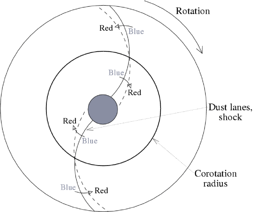
Figure 1: Stellar age gradients across the spiral arms are indicated by arrows that go from blue to red. The azimuthal age gradients are produced by stars born in the spiral shock, where the shocked interstellar medium forms a dust lane, that later drift away as they age. The direction of the gradients changes at the corotation radius, $R_{\rm CR}$. Inside this radius, the disk material overtakes the spiral wave, and beyond it the spiral wave catches up with the material [see also figure 1 in Puerari & Dottori (1997)].

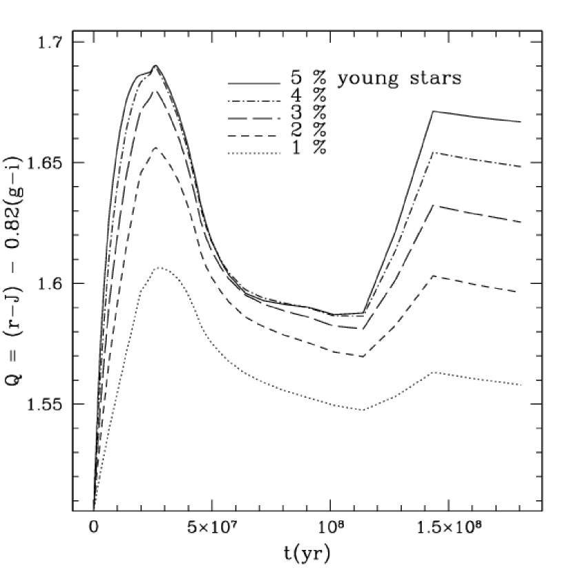
Figure 2: Theoretical $Q(rJgi)$ vs. time, CB07 models. The duration of the burst is $2\times 10^{7}$ years, with a Salpeter IMF; the fraction of young stars ranges from 1% to 5% by mass. Lower and upper mass limits are 0.1 and 10 $M_{\sun}$, respectively.

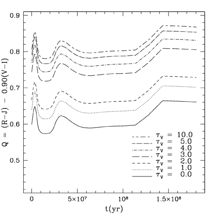
Figure 3: Model Johnson filter $Q(RJVI)$ vs. time $(t)$ for CB07 models, reddened as per the “starburst galaxy” model of Witt et al. (1992). The duration of the burst is $2\times 10^{7}$ years, with a Salpeter IMF and 2% by mass of young stars. Lower and upper mass limits are 0.1 and 100 $M_{\sun}$, respectively.

González & Graham (1996, GG96 hereafter) used for the first time a supergiant sensitive and reddening-free photometric index to trace star formation, defined as:

$$Q(rJgi)=(r-J)-\frac{E(r-J)}{E(g-i)}(g-i).$$ (1)

Using the extinction curves of Schneider et al. (1983), and Rieke & Lebofsky (1985) for a foreground screen, the color excess term is $E(r-J)/E(g-i)=0.82$. According to population synthesis models, following a star formation burst the $Q(rJgi)$ photometric index increases its value for $\sim 2.6\times 10^{7}$ years, and then starts to decline, as shown in Fig. 2 for most recent Charlot & Bruzual (2007, in preparation, CB07 hereafter) models with different stellar mixtures in which young stars constitute from 1% to 5% by mass. Dust lanes arising from spiral shocks are expected to precede the azimuthal color gradients, hence the importance of reddening-free diagnostics. With the stellar population synthesis (SPS) models of Bruzual & Charlot (1993), and the radiative transfer models of Bruzual, Magris & Calvet (1988) and Witt et al. (1992), GG96 investigated the behavior of $Q(RJVI)$ for mixtures of dust and stars with different relative spatial distributions. The main effect of a mixture of dust and stars on the $Q$ index, illustrated in Fig. 3 for the CB07 population synthesis models, is to increase its value relative to the $\tau=0$ and foreground dust screen cases, and $Q(RJVI)$ is no longer reddening-free when $\tau_{V}>2$. However, the requirement that $\tau_{V}<2$ is likely fulfilled by the disks of nearly face-on galaxies (Peletier et al., 1995; Kuchinski et al., 1998; Xilouris et al., 1999); moreover, as stars age, dust dissipates, and reddening diminishes (e.g., Charlot & Fall, 2000).

Based on their study of M 99, GG96 propose that real data are best matched by SPS models with 0.5% to 2%, by mass, of young stars. These values are in accordance with the amount of $B$ light in the arms contributed by young stars, as estimated by Schweizer (1976). GG96 also hypothesize there is an inverse correlation between high-mass star-forming regions and detectable azimuthal color gradients. The color gradient in M 99 lies where no HII regions are identified in $H\alpha$ images of the galaxy. This counterintuitive finding could help explain the dearth of positive detections to date, if contamination from bright emission lines produced in HII regions around the most massive stars masks the color gradients associated with star formation in spiral shocks (Shu, 1997). On the other hand, evidence has been found recently of star forming regions with very few massive stars that generate only scant $H\alpha$ emission (Indebetouw et al., 2008). In this investigation we apply the GG96 method, using the $Q(rJgi)$ photometric index, to a new sample of galaxies in order to search for and analize color-age gradients near spiral arms.

1.1 Color gradients: the link between star formation and spiral dynamics.

According to various studies, spiral density waves must propagate between orbital resonances (Lin, 1970; Mark, 1976; Lin & Lau, 1979; Toomre, 1981; Contopoulos & Grosbøl, 1986). Of these resonances, the most important ones are the inner Lindblad resonance (ILR), the 4:1 resonance, corotation (CR), and the outer Lindblad resonance (OLR).

Azimuthal color-age gradients retain some information about the stellar drift relative to the spiral shock, allowing us to obtain $\Omega_{p}$, the angular velocity of the spiral pattern. In order to find $\Omega_{p}$ from the gradient information, we can use:

$$\Omega_{p}=\frac{1}{t}\left(\int_{0}^{t}\frac{\vec{v}(t^{\prime})\cdot\hat{\varphi}(t^{\prime})}{R(t^{\prime})}\mathrm{d}t^{\prime}-\left(\theta_{\rm shock}+\Delta\theta\right)\right),$$ (2)

$$\Delta\theta=\cot(-i)\ln\left(\frac{R(t)}{R(0)}\right),$$ (3)

where $t$ is the age of the young stellar population at an angle $\theta_{\rm shock}$ away from the shock position ($t^{\prime}$ is a variable of integration), $\vec{v}(t^{\prime})$ is the velocity vector of the young stellar population in an inertial reference system; $\hat{\varphi}(t^{\prime})$ is the unit vector in plane polar coordinates $\rho$, $\varphi$, in a non inertial reference system; $R(t^{\prime})$ is the orbital radius of the studied region, measured from the center of the disk to the center of mass of the young stellar population; and $i$ is the arm pitch angle, if the azimuthal angle increases in the direction of rotation and the spiral arms trail. The angular quantity $\Delta\theta$ accounts for the logarithmic spiral shape of the shock. Assuming the departures from circular motion are small, we have:

$$\Omega_{p}=\frac{1}{R_{mean}}\left(\frac{\int_{0}^{t}v_{rot}(t^{\prime})\mathrm{d}t^{\prime}}{t}-\frac{d}{t}\right),$$ (4)

where $R_{mean}$ is the mean orbital radius of the studied region, $v_{rot}$ is the circular orbital velocity in an inertial reference system, and $t$ is the age of the young stellar population at the azimuthal distance $d$ from the shock. Expanding the term $\int_{0}^{t}v_{rot}(t^{\prime})\mathrm{d}t^{\prime}$, in a Taylor series, we get :

$$\Omega_{p}=\frac{1}{R_{mean}}\left(\frac{(v_{rot})|_{0}t+\frac{1}{2}(\frac{\mathrm{d}v_{rot}}{\mathrm{d}t^{\prime}})|_{0}t^{2}+\zeta}{t}-\frac{d}{t}\right),$$ (5)

where $\zeta$ represents higher order terms in the expansion. According to theory (e.g., Roberts, 1969; Slyz et al., 2003), the higher order terms may account for 20-30 km s^-1, a quantity that is of the same order as the mean rotation velocity error, after considering the uncertainty due to galaxy inclination (see Table 3). Hence, we can neglect the higher order terms in eq. 5, such that $v_{rot}\sim$ constant, and obtain

$$\Omega_{p}\cong\frac{1}{R_{mean}}\left(v_{rot}-\frac{d}{t}\right).$$ (6)

$\Omega_{p}$ is found by stretching the model (which gives $Q$ as a function of $t$) to fit the data (where $Q$ is a function of $d$).

2 Observations and data reduction.

Our total sample of objects consists of 31 almost face-on spiral galaxies of various Hubble types, with angular diameters between $4\arcmin$ and $6\arcmin$. This sample was chosen from the Uppsala general catalogue of galaxies (UGC; Nilson, 1973), the ESO-Uppsala survey of the ESO (B) atlas (Lauberts, 1982), and the Second reference catalogue of bright galaxies (de Vaucouleurs et al., 1976). From this sample, we further select for their analysis in the present paper 13 A and AB (de Vaucouleurs, 1959) galaxies, based on the visual inspection of their 2-D images in the $Q(rJgi)$ photometric index. In this diagnostic, the disks of some of the galaxies in our original sample of 31 clearly appear divided in two halves, each one with a different average value of $Q$. The analysis of these “$Q$ effect” galaxies and of the remaining barred galaxies will be undertaken in subsequent publications.

The data were acquired during 1992-1995 with four different telescopes: the Lick Observatory 1-m, the Kitt Peak National Observatory (KPNO) 1.3-m, and the Cerro Tololo Interamerican Observatory (CTIO) 0.9-m and 1.5-m telescopes. Deep photometric images were taken in the optical filters $g$, $r$, and $i$, and in the near-IR $J$, $K_{s}$ (Persson et al., 1998) or $K^{\prime}$ (Wainscoat & Cowie, 1992). Effective wavelengths and widths of all the filters are listed in Table 1; the observation log for the 13 galaxies is shown in Table 2.

Table 1: Filter characteristics

Filter	$\lambda_{eff}$	FWHM
$g$	5000Å	830Å
$r$	6800Å	1330Å
$i$	7800Å	1420Å
$J$	1.25µm	0.29µm
$K_{s}$	2.16µm	0.33µm
$K^{\prime}$	2.11µm	0.35µm

The CCD at the Lick 1-m telescope was a Ford $2048^{2}$, with a pixel scale of $0\farcs 185$ pixel^-1. For the infrared observations at Lick, the same telescope was fitted with the LIRC-2 camera; it had a $256^{2}$ NICMOS II detector, with a $1\farcs 145$ pixel^-1 plate scale. The CTIO 0.9-m optical telescope used a Tek $1024^{2}$ and a Tek $2048^{2}$ CCDs, both with a $0\farcs 4$ pixel^-1 plate scale. The CTIO infrared observations were performed at the 1.5-m telescope, with the CIRIM instrument, which used a $256^{2}$ NICMOS3 array; the CIRIM focus was adjusted to give a $1\farcs 16$ pixel^-1 plate scale. The KPNO infrared observations were made with the IRIM camera, that employed a $256^{2}$ NICMOS3 array, with a $2\arcsec$ pixel^-1 plate scale.

The data were reduced with the image processing package IRAF (Tody, 1986, 1993), using standard techniques. For the optical data, overscan and trimming corrections were first applied. Bias subtraction and flat field division corrections were used. Master flats were produced from stacks of twilight flats that were averaged pixel by pixel, after scaling each flat by its median value and sigma-clipping deviant pixels; the master flats were then divided by their mean pixel value. For sky subtraction, the sky level was determined by masking bright objects in the image and subsequently fitting a constant value to the remaining pixels, after rejection iterations. To produce mosaics, individual frames were superpixelated by a factor of 2 in each dimension, and registered to the nearest half (original) pixel. Before adding into the final mosaic, cosmic rays were removed by comparing each individual image with a median one.

A correction for non-linearity was applied to the near-IR data. The correction was obtained by adjusting a polynomial function, pixel by pixel, to dome flats of increasing exposure times, taking into account variations in the count-rate between exposures. During observations, frames were mostly taken in the sequence SKY-SKY-OBJECT-OBJECT-SKY-SKY… Objects in the sky were masked, and the sky frames were median scaled, averaged, and subtracted from the object. This procedure also takes care of dark current removal. Flat field corrections were applied with master flats derived from dome flats. Cosmic ray removal and mosaic registering were done with the same procedure used for the optical data.

The optical calibration was performed using synthetic photometry in the Thuan-Gunn system (Thuan & Gunn, 1976; Wade et al., 1979). This system is based on the standard star BD+17$\arcdeg$4708, to which the magnitude $g=9.5$, and the color indices $g-r=r-i=0$ are assigned. Synthetic magnitudes for other spectrophotometric standards were obtained by means of the following relation:

$${\rm mag}_{syn}=-2.5\log_{10}\left(\frac{\int_{0}^{\infty}f_{\lambda}R(\lambda)d\lambda}{\int_{0}^{\infty}R(\lambda)d\lambda}\right)+ZP,$$ (7)

where $f_{\lambda}$ is the absolute spectral energy distribution of the star in ergs s^-1 cm^-2 ${\rm\AA}^{-1}$; $ZP$ is the zero point, and $R(\lambda)$ is the system response curve, including the quantum efficiency of the detector, the transmission function of the filter, and the effect of atmospheric absorption. The atmospheric transmission curve for the northern hemisphere observations was taken from Hayes (1970), and for CTIO from Hamuy et al. (1992). The absolute fluxes were obtained, for BD+17$\arcdeg$4708 from Oke & Gunn (1983), and for the remaining standard stars from Stone (1977), Massey et al. (1988), Massey & Gronwall (1990), Hamuy et al. (1992), and Hamuy et al. (1994). Individual galaxy frames taken under photometric conditions were used for calibration, and mosaics were scaled to such photometric data.

For the infrared data, we only had one photometric season at KPNO and none at CTIO. In order to obtain a uniform photometry, we calibrated our $J$ and $K_{s}$ data with images from the Two Micron All Sky Survey (2MASS, Skrutskie et al., 1997, 2006). For the $K^{\prime}$ data, we use photometric standards from Hawarden et al. (2001), and adopt $K^{\prime}=K+0.2(H-K)$ (Wainscoat & Cowie, 1992). We do not include color correction terms in our infrared calibration, but take this systematic error into account in the zero point uncertainty.

Finally, the optical images were degraded to the lower resolution of the infrared images, and aligned with them in order to proceed.

Table 2: Observation Log

Object	Filter	Exposure(s)	Telescope	Date (month/year)
NGC 4939 ……	$g$	2700.	CTIO 0.9 m	3/94
	$g$	300.	Lick 1 m	4/94
	$r$	2400.	CTIO 0.9 m	3/94
	$r$	300.	Lick 1 m	4/94
	$i$	3600.	CTIO 0.9 m	3/94
	$i$	300.	Lick 1 m	4/94
	$J$	840.	Kitt Peak 1.3 m	3/94
	$K_{s}$	515.	”	”
NGC 3938 ……	$g$	600.	Lick 1 m	4/94
	$r$	300.	”	”
	$i$	1189.	”	2/94, 4/94
	$J$	1252.	Lick 1 m	2/95
	$J$	600.	Kitt Peak 1.3 m	3/94
	$K_{s}$	560.	”	”
NGC 4254 ……	$g$	4443.	Lick 1 m	4/94
	$r$	2100.	”	”
	$i$	3308.	”	”
	$J$	501.	Lick 1 m	2/95
	$J$	960.	Kitt Peak 1.3 m	3/94, 11/94
	$K_{s}$	590.	”	”
NGC 7126 ……	$g$	3900.	CTIO 0.9 m	9/94
	$r$	3900.	”	”
	$i$	3900.	”	”
	$J$	300.	CTIO 1.5 m	9/95
	$K_{s}$	390.	”	9/95
NGC 1417 ……	$g$	3600.	Lick 1 m	9/93, 10/93
	$r$	5048.	”	9/93, 10/93, 11/93
	$i$	3600.	”	9/93, 10/93
	$J$	720.	Kitt Peak 1.3 m	9/93
	$K_{s}$	256.	”	”
NGC 7753 ……	$g$	4500.	Lick 1 m	11/93, 10/94, 11/94
	$r$	5812.	”	”
	$i$	5307.	”	”
	$J$	626.	Lick 1 m	10/94
	$K^{\prime}$	113.4	”	”
NGC 6951 ……	$g$	6120.	Lick 1 m	6/92, 8/92, 9/93
	$r$	6900.	”	”
	$i$	6296.	”	7/92, 8/92, 9/93
	$J$	2136.	Lick 1 m	9/93, 11/94
	$J$	4140.	Kitt Peak 1.3 m	7/94
	$K_{s}$	608.	”	9/93, 11/94
NGC 5371 ……	$g$	5100.	Lick 1 m	6/92, 3/93, 4/94
	$r$	6600.	”	”
	$i$	2375.	”	6/92, 4/94
	$J$	501.	Lick 1 m	2/95
	$J$	870.	Kitt Peak 1.3 m	3/94
	$K_{s}$	520.	”	”
NGC 3162 ……	$g$	5400.	Lick 1 m	3/93, 11/93, 4/94, 10/94, 11/94
	$r$	6000.	”	4/93, 11/93, 4/94, 10/94, 11/94
	$i$	1800.	”	11/93, 4/94, 10/94, 11/94
	$J$	990.	Kitt Peak 1.3 m	3/94
	$K_{s}$	560.	”	”
NGC 1421 ……	$g$	3600.	CTIO 0.9 m	9/94
	$r$	3600.	”	”
	$i$	3550.	”	”
	$J$	2241.	Lick 1 m	10/94, 12/94
	$J$	330.	CTIO 1.5 m	9/94
	$J$	300.	Kitt Peak 1.3 m	11/94
	$K_{s}$	160.	CTIO 1.5 m	9/94
	$K_{s}$	60.	Kitt Peak 1.3 m	11/94
NGC 7125 ……	$g$	3900.	CTIO 0.9 m	9/94
	$r$	3900.	”	”
	$i$	3900.	”	”
	$J$	600.	CTIO 1.5 m	9/95
	$K_{s}$	285.	”	”
NGC 918 ……	$g$	4500.	Lick 1 m	11/93, 10/94, 11/94
	$r$	4500.	”	”
	$i$	5400.	”	”
	$J$	2567.	Lick 1 m	10/94, 12/94
	$K^{\prime}$	897.6	”	”
NGC 578 ……	$g$	3900.	CTIO 0.9 m	9/94
	$r$	3600.	”	”
	$i$	4800.	”	”
	$J$	240.	CTIO 1.5 m	9/95
	$K_{s}$	375.	”	”

Prior to analysis proper, the images were deprojected using position angles ($P.A.$) and isophotal diameter ratios taken from the Third Reference Catalogue of Bright Galaxies (RC3, de Vaucouleurs et al., 1991), unless indicated otherwise in Table 3. The inclination angle ($\alpha$) was obtained using the simple approximation $\cos\alpha=(b/a)$.

The spiral arms where then unwrapped by plotting them in a $\theta$ vs. ln $R$ map (Iye et al., 1982; Elmegreen et al., 1992). Under this geometric transformation, logarithmic spirals appear as straight lines with slope = cot(-$i$), where $i$ is the arm pitch angle. Following the procedure used by GG96, the phase of $\theta$ was then changed for each (fixed) value of ln $R$, until the arms appeared horizontal. This way, selected regions with candidate color gradients can be easily collapsed in ln $R$ to yield 1-D plots of intensity vs. distance; features in such plots have a higher signal-to-noise ratio than in 2-D images, and can be directly compared to the SPS models.

Table 3: Galaxy parameters

Name	Type	P.A. (degrees)	$a/b$	$v_{max}$ (km s-1)	Radial velocity (km s-1)	Distance (Mpc)
NGC 4939	SA(s)bc	10	$1.95\pm 0.13$	$207.5\pm 7.6$	$3111\pm 5$	$46.5\pm 4.0$
NGC 3938	SA(s)c	52	$1.10\pm 0.05$	$39.2\pm 3.6$	$809\pm 4$	$15.8\pm 1.4$
NGC 4254	SA(s)c	68	$1.15\pm 0.05$	$106.7\pm 6.4$	$2407\pm 3$	$16.5\pm 1.1$
NGC 7126	SA(rs)c	80	$2.19\pm 0.15$	$152.4\pm 2.8$	$3054\pm 8$	$44.6\pm 3.8$
NGC 1417	SAB(rs)b	10	$1.62\pm 0.11$	$205.1\pm 4.3$	$4120\pm 17$	$57.1\pm 4.8$
NGC 7753	SAB(rs)bc	50	$1.58\pm 0.15$	$164.8\pm 9.5$	$5163\pm 4$	$72.1\pm 6.1$
NGC 6951	SAB(rs)bc	170	$1.20\pm 0.08$	$144.2\pm 6.0$	$1426\pm 6$	$24.9\pm 2.1$
NGC 5371	SAB(rs)bc	8	$1.26\pm 0.09$	$177.0\pm 11.8$	$2553\pm 7$	$43.5\pm 3.7$
NGC 3162	SAB(rs)bc	31	$1.20\pm 0.08$	$76.6\pm 7.8$	$1298\pm 7$	$23.7\pm 2.1$
NGC 1421	SAB(rs)bc	0	$4.07\pm 0.28$	$165.9\pm 8.8$	$2090\pm 5$	$29.3\pm 2.5$
NGC 7125	SAB(rs)c	110	$1.45\pm 0.10$	$104.2\pm 18.2$	$3054\pm 8$	$44.6\pm 3.8$
NGC 918	SAB(rs)c	158	$1.70\pm 0.16$	$112.5\pm 6.2$	$1509\pm 4$	$21.7\pm 1.8$
NGC 578	SAB(rs)c	110	$1.58\pm 0.07$	$117.8\pm 4.1$	$1630\pm 4$	$22.7\pm 1.9$

Note. — Col. (2) and (3). Types and position angles from RC3. Col. (4). Isophotal diameter ratio derived from the $R_{25}$ parameter in RC3. Col. (5). Maximum rotation velocity obtained from the HI data of Paturel et al. (2003), not corrected for inclination. Col. (6). Heliocentric radial velocity from RC3. Col. (7). Hubble distance obtained from the heliocentric radial velocity and the infall model of Mould et al. (2000).

3 The $Q(rJgi)$ photometric index and the stellar population synthesis models.

With the aim of tracing star formation across the spiral arms of disk galaxies we use the $Q(rJgi)$ reddening-free photometric index, as defined by GG96. The $Q(rJgi)$ index was chosen between different possible filter combinations for two reasons: (1) the quotient of relevant color excesses is close to unity, and hence all bands involved have similar weights, and (2) because the SPS models (e.g., Bruzual & Charlot, 2003) predict a detectable gradient. To explain how $Q$ works, GG96 express it in logarithmic form:

$$Q(rJgi)=\log_{10}\frac{I^{2.05}_{g}I^{2.50}_{J}}{I^{2.50}_{r}I^{2.05}_{i}},$$ (8)

where $I_{x}$ is the light intensity in each filter. In active star forming regions, blue and red supergiants dominate the scene, and the $Q(rJgi)$ index has higher values because the $g$ and $J$ bands in the numerator of eq. 8 are tracing, respectively, the light from these stars. Conversely, when star formation activity is poor, the $Q(rJgi)$ index has a relative lower value.

For the present work, we use a preliminary version of the CB07 models for comparison with the observations. A star formation burst was added to a background population of old stars with an age of $5\times 10^{9}$ years; both components have a Salpeter IMF. Using an older background population makes no difference in $Q(rJgi)$. The burst has a duration of $2\times 10^{7}$ years, in accordance with the age spread of OB associations inferred from observations (e.g., Elmegreen & Lada, 1977; Doom et al., 1985; Massey et al., 1989; Burningham et al., 2005).

Each of the four bands needed to produce the model $Q(rJgi)$ index was calculated as shown below for $g$:

$$g_{\rm csp}(t)=-2.5\log_{10}(\beta_{I}10^{-0.4g_{\rm yng}(t)}+\beta_{II}10^{-0.4g_{\rm old}}),$$ (9)

where $g_{\rm csp}(t)$ is the $g$-band surface brightness, in mag arcsec^-2, of the composite model stellar population (csp) made up of young and old stars, at time $t$ after the formation of the young stars. $\beta_{I}$ and $\beta_{II}$ are, respectively, the fractions of young and old stars by mass ($\beta_{II}=1-\beta_{I}$); $g_{\rm yng}(t)$ is the $g$ surface brightness of the young single stellar population at time $t$; and $g_{\rm old}$ is the $g$-band surface brightness of the old single stellar population. The same holds for the $r$, $i$, and $J$ bands.

4 Results.

For the time being, we adopt models with constant stellar velocity (i.e., stellar orbits are assumed to be circular) and with a constant fraction of young stars of 2% by mass. IMF upper mass limits of both 10 and 100 $M_{\sun}$ are considered. No data were matched by the models with $M_{upper}=100M_{\odot}$, however. We also use models with solar metallicity in both populations, and shift them to the surface brightness level observed from the data for each object. A possible reason for the need of this shift is metallicity, as will be explained in § 5.3. The rigorous application of more complex models would require an individual treatment of each galaxy and region.

Once $\Omega_{p}$ is known, it is possible to locate major resonances in the galaxy deprojected images, thus providing a link between the color gradients and the dynamics of the spiral disk. That is, if the gradients are indeed caused by star formation in large-scale shocks, the positions of the spiral endpoints must be consistent with the location of major resonances, as deduced from a comparison between the derived $\Omega_{p}$ and the known orbital velocity.

There are rotation curves available in the literature for a few objects in our sample, but observed with different criteria. With the purpose of homogenizing our sample, we use the HI data of Paturel et al. (2003), who give the maximum rotation velocity uncorrected for inclination. These values are shown in Table 3. An important aspect to notice in equation 6 is that $R_{mean}$, $v_{rot}$, and $d$ depend on the inclination angle $\alpha$ used to deproject the images. An independent variable form of this equation is shown in the Appendix (see equation A1), which we use to obtain the uncertainty in $\Omega_{p}$. Also, in order to determine $\Omega_{p}$, the distance to the object must be known. We use the model of Mould et al. (2000) to convert galaxy heliocentric velocities, obtained from the RC3 catalogue, to Hubble flow velocities; from these we find the distance, adopting H${}_{0}=71\pm 6$ km s^-1 Mpc^-1 (Mould et al., 2000). At small redshift, the uncertainty in the model is expected to be $\sim 100$ km s^-1. The uncertainty for any single galaxy is about 100 km s^-1, plus the field dispersion (perhaps as big as 250 km s^-1, and much larger in cluster cores), added in quadrature. The model works well for groups and clusters locally, and less well (by definition) for individual galaxies, unless they are in a quiet part of the flow (Huchra, J. P. 2008, private communication). The heliocentric velocities for our objects and the distances derived from this model are shown in Table 3. To obtain the distance uncertainty we propagate the errors of the heliocentric and infall velocities in the equations of the Mould et al. model.

All the spiral arms visible in the mosaics were inspected for profiles similar to those expected from azimuthal color gradients. Only a few regions across the arms of the analyzed objects present profiles that match the theoretical expectations. These regions are marked in the optical mosaics of each individual object. The $Q(rJgi)$ index data, tracing star formation; the $(g-J)$ data, outlining the dust lane location, and the $K_{s}$ (or $K^{\prime}$) data, following the density wave, are shown for each single region. The site with the highest $(g-J)$ value (i.e., the highest extinction) is taken as the origin of the (azimuthal) distance (in kpc), which increases in the sense of rotation; the direction of rotation was inferred assuming that arms are trailing. The comparison between model and data $Q(rJgi)$ index is shown in separate figures, where the vertical error bars correspond to $\pm 1\sigma$ of the computed uncertainty in $Q$, including read-out noise and sky subtraction. The horizontal bars represent the uncertainty in the “stretch” applied to the the model in order to fit the data. This is ultimately an uncertainty in the stellar drift velocity and, hence, in $\Omega_{p}$, and is obtained as explained in the Appendix. We include in this error an estimate of the different stretch that would be required by models with variable densities, velocities and metallicities discussed in § 5 (see figure 11). The resonance locations determined once $\Omega_{p}$ was obtained from stretching the stellar population model to the data are marked on the infrared mosaics. The observed parameters for each region and the derived dynamic ones are summarized in Table 4. The $Q$ index magnitude offset, applied to the solar metallicity model with 2% of young stars in order to fit the data, is also listed.

From our $K_{s}$ and $K^{\prime}$ data we obtain visually the location of the spiral endpoints in our objects. In some few cases the signal-to-noise ratio was too low, and the $J$ or the optical $i$ images were used instead. The positions of the derived spiral endpoints, as well as the wavelength used, are listed in Table 4. We compare these spiral endpoints with the locations of major resonances (4:1 resonance, corotation, and OLR) inferred from the $Q(rJgi)$ index data and the stellar models, as described in § 1.1. For objects with more than one studied region we choose the one with the lowest uncertainty and the best match with the spiral endpoints. The selected regions are marked with an asterisk in Table 4. The results of this analysis are summarized in Fig. 4; the vertical axis corresponds to the $R_{res}/R_{end}$ ratio, where $R_{res}$ is the location of the major resonance derived from the analysis, and $R_{end}$ is the spiral endpoint obtained from the data.

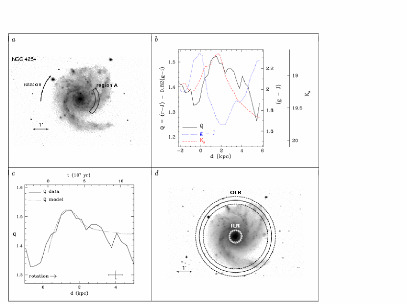
Figure 18: Region NGC 4254 A. Panel $a$: Deprojected spiral galaxy NGC 4254 in the optical $g$-band. The display is in logarithmic scale. The studied regions are marked on the figure. Panel $b$: 1-D data vs. azimuthal distance for region NGC 4254 A. Solid line: $Q$ index; dotted line: ($g-J$) color; dashed line: $K_{s}$-band profile. Panel $c$: Zoom-in of region, and 1-D $Q$ index vs. azimuthal distance. Solid line: data; dotted line: model. Data error bars and direction of rotation are indicated. Panel $d$: $K_{s}$-band deprojected mosaic of spiral galaxy NGC 4254. Solid line circles: location of the ILR and the OLR, as obtained from the comparison between data and stellar population SPS model shown in panel $c$. Dashed line circles: $\pm 1\sigma$ errors.

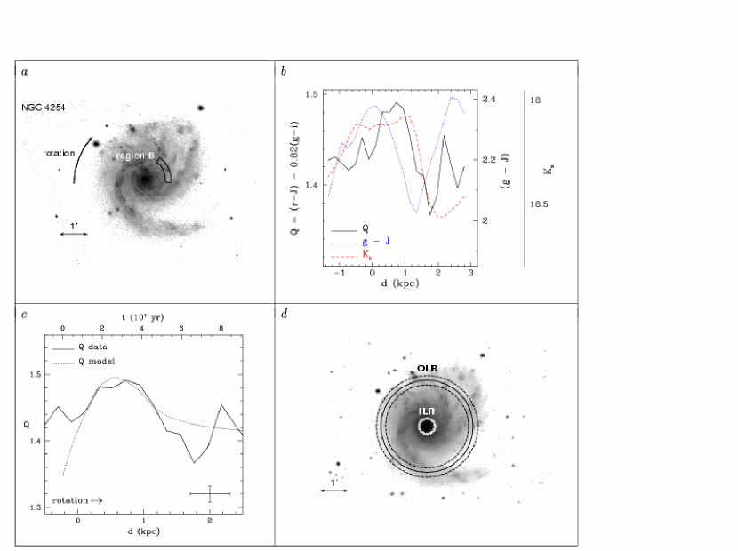
Figure 19: Region NGC 4254 B.

With the exception of NGC4254 (M 99), objects are organized by Hubble type (from SAbc to SABc). Remarks in the caption of Fig. 18 apply also to figures 19 – 41, unless indicated in individual captions.

NGC 4254 : [Figures 18 - 19] Although NGC 4254 is a “$Q$ effect” galaxy with two asymmetric halves in this diagnostic, we include it here as a test of the consistency of our procedure vis-à-vis its first application by GG96. The resonance positions computed for region NGC 4254 A (the same analyzed by GG96) place the spiral endpoint for the corresponding arm at the OLR. Even though the $\Omega_{p}$ for region NGC 4254 B differs from the value obtained for region A, the spiral endpoint of the arm to which this region belongs matches the position of its OLR too! Not surprisingly for a “$Q$ effect” galaxy, region B $Q$ values are also 0.03 magnitudes below those for region A. Given the fact that the two gradients yield different values for $\Omega_{p}$ but their corresponding arms end at their respective OLR, we hypothesize that the “$Q$ effect” is related to the dynamics of the disk.

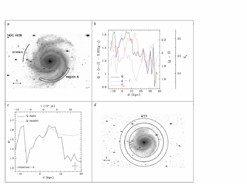
Figure 21: Region NGC 4939 A. In order to fit the model to the data we assume now that the gradient occurs inside corotation. In this case, time evolution (top axis in panel $c$) and rotation have the same direction. Panel $d$, solid line circle: location of the 4:1 resonance, as obtained from the comparison between data and SPS model shown in panel $c$.

NGC 4939 : [Figures 20 - 21] From the location of the dust lanes in this region, it is hard to determine the age gradient direction and hence whether it occurs inside or outside corotation. If one assumes it is outside corotation (inverse gradient), the spiral endpoints are located near the OLR, as shown in Fig. 20. If, contrariwise, one assumes the age gradient is inside corotation, the spiral endpoints may coincide with the location of the 4:1 resonance (see Fig. 21). Region NGC 4939 A has a shape that differs from the models, a fact that could be explained if the galaxy metallicity is different from the one assumed (see § 5.3).

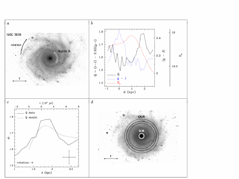
Figure 22: Region NGC 3938 A. Panel $a$: Deprojected spiral galaxy NGC 3938 in the optical $r$-band.

NGC 3938 : [Figure 22] The signal-to-noise ratio for the optical images of this galaxy is lower than for other objects in the sample. The dynamical parameters inferred from the data yield resonance positions that do not match the location of the spiral endpoints.

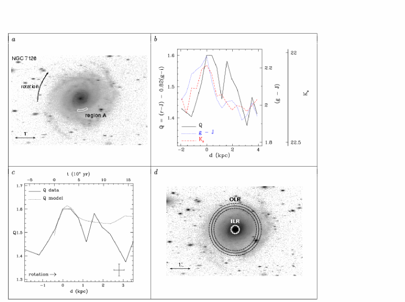
Figure 23: Region NGC 7126 A. Panel $d$: $i$-band deprojected mosaic of spiral galaxy NGC 7126.

NGC 7126 : [Figure 23] The inferred locations of major resonances do not match any spiral endpoint in the $K_{s}$ mosaic, which has a low signal-to-noise ratio. However, in the $i$-band mosaic two well defined spiral arms can be seen that extend beyond the position of the OLR. We conclude that the gradient featured in region NGC 7126 A may not be due to star formation triggered by the spiral shock.

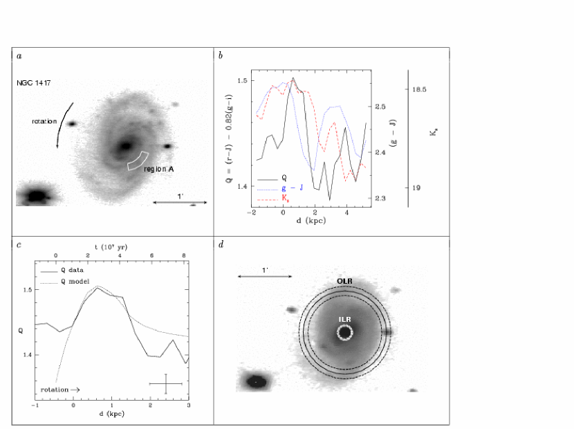
Figure 24: Region NGC 1417 A. Panel $d$: $J$-band deprojected mosaic of spiral galaxy NGC 1417.

NGC 1417 : [Figures 24 - 26] Regions A, B, and C for NGC 1417 give the same corotation position (8 kpc) within the errors (see Table 4). The spiral arms end at the OLR.

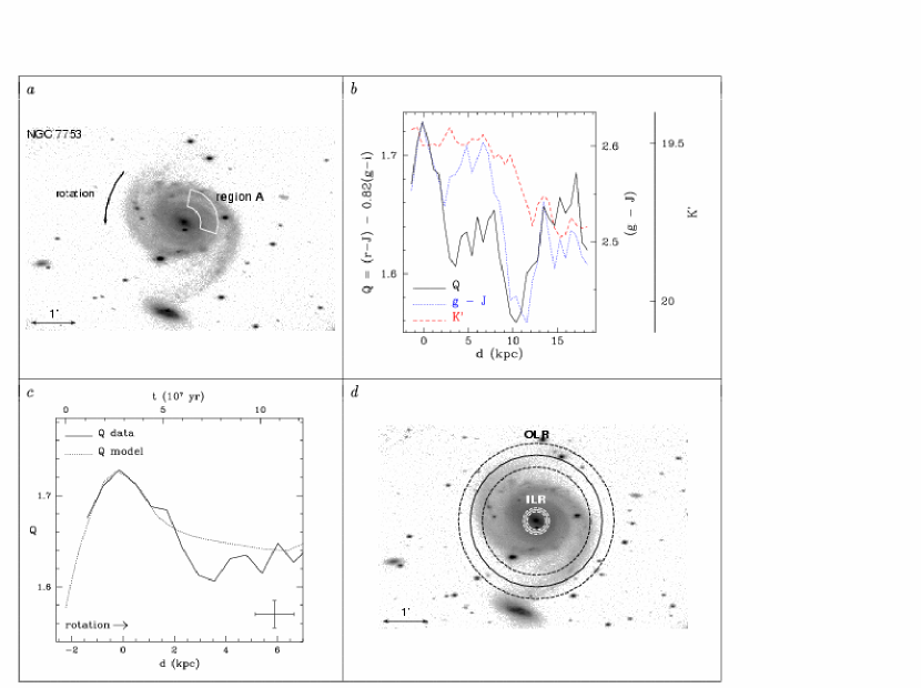
Figure 27: Region NGC 7753 A. Panel $d$: $i$-band deprojected mosaic of spiral galaxy NGC 7753.

NGC 7753 : [Figure 27] Apparently, the gradient studied in this object coincides with a dust lane feature. Nevertheless, according to the computed $\Omega_{p}$, the spiral endpoints match the OLR within the errors.

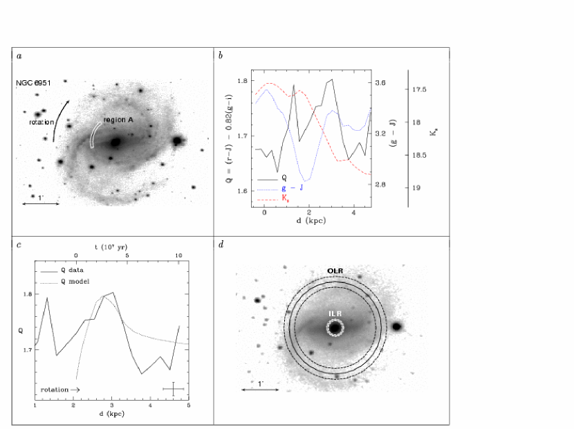
Figure 28: Region NGC 6951 A.

NGC 6951 : [Figure 28] Neither of the resonance positions computed from the data of region NGC 6951  A matches the spiral endpoints.

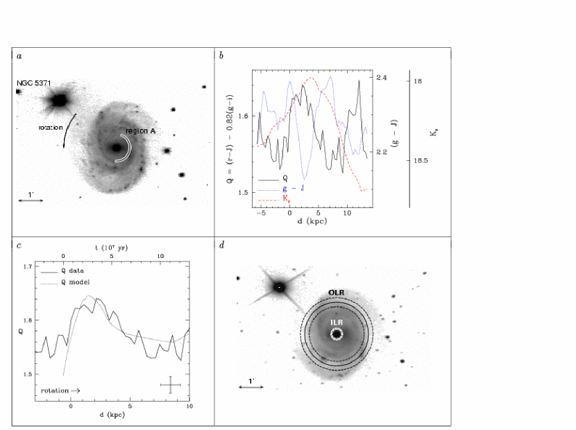
Figure 29: Region NGC 5371 A.

NGC 5371 : [Figures 29 - 30] The dynamic parameters derived for regions A and B result in different locations of the major resonances. Those for region A do not coincide with the spiral endpoints of the object. However, region B yields an OLR position that matches the spiral endpoints.

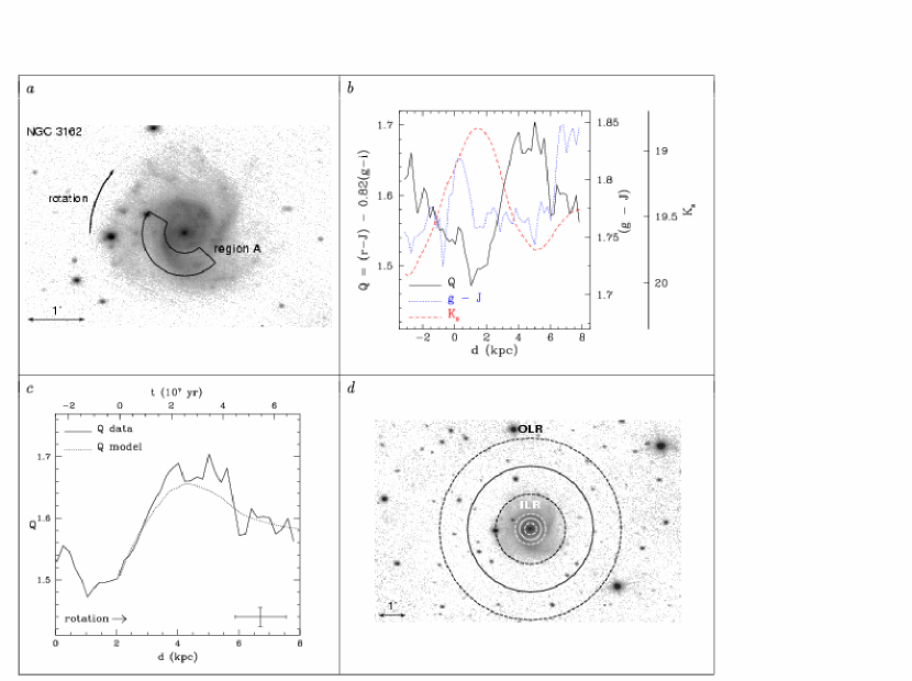
Figure 31: Region NGC 3162 A. Panel $d$: $J$-band deprojected mosaic of spiral galaxy NGC 3162.

NGC 3162 : [Figures 31 - 32] The computed OLR for region B coincides with the the spiral endpoints. The computed errors of the dynamic parameters for region A are larger than for region B.

NGC 1421 : [Figures 33 - 35] Region A has an offset in $Q$ of +0.1 mag when compared to regions B and C. On the other hand, regions A and C give resonance positions that agree with the spiral endpoints; the best match is for region C, which is also an inverse azimuthal color gradient (i.e., situated after corotation). The feature studied in region B must not be caused by star formation linked to the dynamics of the disk.

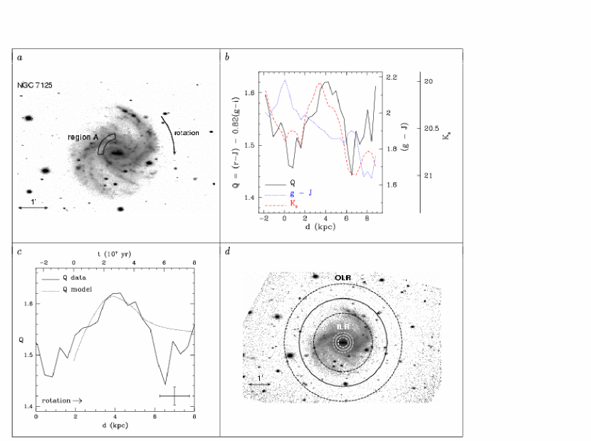
Figure 36: Region NGC 7125 A. Panel $d$: $J$-band deprojected mosaic of spiral galaxy NGC 7125.

NGC 7125 : [Figures 36 - 38] Region B displays an inverse gradient. The results obtained from the three studied regions agree within their errors. The spiral endpoints coincide with the OLR in this object.

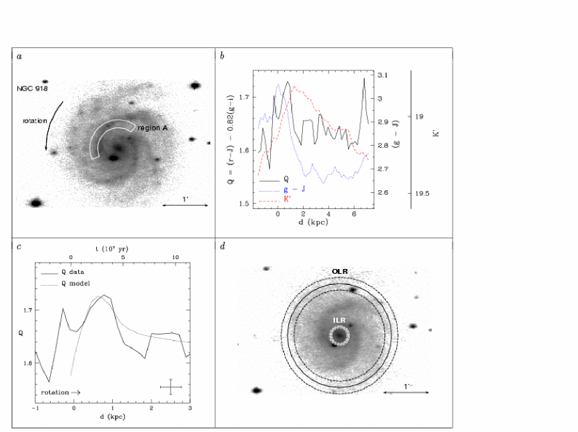
Figure 39: Region NGC 918 A. Panel $d$: $K^{\prime}$-band deprojected mosaic of spiral galaxy NGC 918.

NGC 918 : [Figure 39] The stellar population model stretched to the data from region A indicates that the spiral arms end at the OLR in this galaxy.

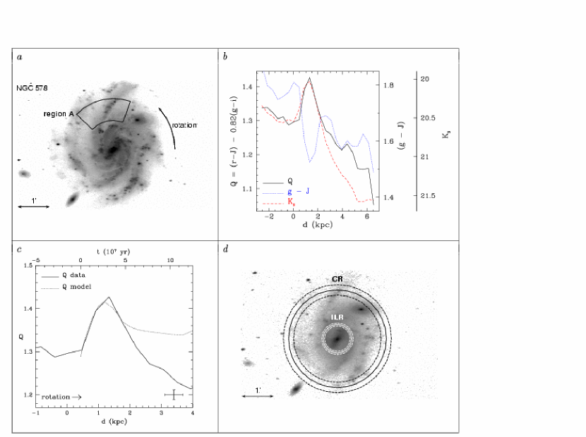
Figure 40: Region NGC 578 A. Panel $d$, solid line circles: location of the ILR and corotation radius, as obtained from the comparison between data and SPS model shown in panel $c$.

NGC 578 : [Figures 40 - 41] Regions A and B, located in two different arms of the four that conform this object, yield the same value for the spiral pattern speed. In the deprojected mosaics, the northern arms, including the one harboring region A, seem to extend beyond the corotation radius without reaching the OLR within the errors. The other arms, where region B is located, end at corotation. This is the only object in the sample that presents spiral arms ending at corotation.

Table 4: Observed and derived dynamic parameters.

Region number	Galaxy and region	$R_{\rm mean}$ (arcsec)	$R_{\bf mean}$ (kpc)	$R_{\rm end}$ (arcsec)	$R_{\bf end}$ (kpc)	$Q_{\bf offset}$ (mag)	$\Omega_{p}$ (km s-1 kpc-1)	$R_{\rm CR}$ (arcsec)	$R_{\rm CR}$ (kpc)
1	NGC4254 A*	$66.4\pm 0.25$	$5.3\pm 0.4$	157.5$\pm$7.5 ($K_{s}$)	12.6$\pm$0.8	$-0.13\pm 0.05$	$33.5\pm 8.2$	$81.0\pm 8.6$	$6.5\pm 0.7$
2	NGC4254 B	$49.3\pm 0.25$	$3.9\pm 0.3$			$-0.16\pm 0.05$	$47.7\pm 11.4$	$57.0\pm 5.6$	$4.6\pm 0.4$
3	NGC4939 A*	$129.4\pm 0.25$	$29.2\pm 2.5$	145$\pm$5 ($K_{s}$)	32.7$\pm$2.8	$0.0\pm 0.06$	$12.3\pm 0.8$	$87.5\pm 5.3$	$19.7\pm 1.2$
4	NGC3938 A*	$30.7\pm 0.25$	$2.3\pm 0.2$	100$\pm$5 ($K_{s}$)	7.7$\pm$0.7	$+0.09\pm 0.06$	$33.8\pm 12.9$	$36.9\pm 5.2$	$2.8\pm 0.4$
5	NGC7126 A*	$34.6\pm 0.15$	$7.5\pm 0.6$	118.9$\pm$2.9 ($i$)	25.7$\pm$2.2	$0.0\pm 0.09$	$19.7\pm 2.2$	$40.2\pm 4.1$	$8.7\pm 0.9$
6	NGC1417 A	$22.6\pm 0.25$	$6.3\pm 0.5$	60$\pm$5 ($J$)	16.6$\pm$1.4	$-0.15\pm 0.06$	$35.1\pm 4.7$	$26.8\pm 2.9$	$7.4\pm 0.8$
7	NGC1417 B*	$25.3\pm 0.25$	$7.0\pm 0.6$			$-0.18\pm 0.06$	$29.9\pm 4.1$	$31.5\pm 3.6$	$8.7\pm 1.0$
8	NGC1417 C	$20.4\pm 0.25$	$5.7\pm 0.5$			$-0.15\pm 0.06$	$33.6\pm 5.2$	$28.1\pm 3.6$	$7.8\pm 1.0$
9	NGC7753 A*	$33.7\pm 0.15$	$11.8\pm 1.0$	95.7$\pm$5.8 ($i$)	33.5$\pm$2.8	$+0.07\pm 0.09$	$11.7\pm 2.8$	$51.7\pm 9.0$	$18.1\pm 3.2$
10	NGC6951 A*	$38.8\pm 0.25$	$4.7\pm 0.4$	105$\pm$5 ($K_{s}$)	12.7$\pm$1.1	$+0.14\pm 0.07$	$49.9\pm 12.8$	$43.2\pm 5.0$	$5.2\pm 0.6$
11	NGC5371 A	$32.2\pm 0.25$	$6.8\pm 0.6$	115$\pm$5 ($K_{s}$)	24.3$\pm$2.1	$-0.01\pm 0.05$	$31.2\pm 7.6$	$44.3\pm 6.1$	$9.3\pm 1.3$
12	NGC5371 B*	$41.8\pm 0.25$	$8.8\pm 0.7$			$+0.03\pm 0.05$	$20.8\pm 6.5$	$66.6\pm 13.3$	$14.0\pm 2.8$
13	NGC3162 A	$33.0\pm 0.25$	$3.8\pm 0.3$	75$\pm$5 ($J$)	8.6$\pm$0.8	$0.0\pm 0.06$	$14.7\pm 8.3$	$81.8\pm 33.5$	$9.4\pm 3.8$
14	NGC3162 B*	$35.7\pm 0.25$	$4.1\pm 0.4$			$0.0\pm 0.06$	$25.0\pm 8.3$	$48.0\pm 7.9$	$5.5\pm 0.9$
15	NGC1421 A	$34.6\pm 0.15$	$4.9\pm 0.4$	92.8$\pm$2.9 ($K_{s}$)	13.2$\pm$1.1	$+0.05\pm 0.09$	$16.6\pm 3.5$	$72.6\pm 13.9$	$10.3\pm 2.0$
16	NGC1421 B	$57.5\pm 0.15$	$8.2\pm 0.7$			$-0.04\pm 0.09$	$0.5\pm 2.2$	$2230.1\pm 15820.0$	$316.8\pm 2247.2$
17	NGC1421 C*	$80.0\pm 0.15$	$11.4\pm 1.0$			$-0.05\pm 0.09$	$22.3\pm 1.7$	$54.0\pm 3.6$	$7.7\pm 0.5$
18	NGC7125 A	$33.6\pm 0.15$	$7.3\pm 0.6$	95.7$\pm$2.9 ($J$)	20.7$\pm$1.8	$0.0\pm 0.09$	$9.6\pm 4.3$	$69.4\pm 22.1$	$15.0\pm 4.8$
19	NGC7125 B*	$79.1\pm 0.15$	$17.1\pm 1.5$			$0.0\pm 0.09$	$10.8\pm 1.7$	$61.7\pm 4.8$	$13.3\pm 1.0$
20	NGC7125 C	$45.3\pm 0.15$	$9.8\pm 0.8$			$-0.02\pm 0.09$	$9.8\pm 3.2$	$68.5\pm 12.6$	$14.8\pm 2.7$
21	NGC918 A*	$32.1\pm 0.15$	$3.4\pm 0.3$	75.4$\pm$5.8 ($K^{\prime}$)	7.9$\pm$0.7	$+0.07\pm 0.05$	$33.4\pm 5.7$	$39.6\pm 4.9$	$4.2\pm 0.5$
22	NGC578 A*	$75.2\pm 0.15$	$8.3\pm 0.7$	95.7$\pm$2.9 ($K_{s}$)	10.5$\pm$0.9	$-0.2\pm 0.09$	$15.0\pm 1.9$	$92.2\pm 9.7$	$10.1\pm 1.1$
23	NGC578 B	$67.8\pm 0.15$	$7.5\pm 0.6$			$-0.16\pm 0.09$	$15.2\pm 2.2$	$90.8\pm 10.9$	$10.0\pm 1.2$

Note. — Col. (3) and (4). Mean radius of the studied regions, in arcsec and kpc, respectively. Col. (5) and (6). Radius of the spiral endpoint, in arcsec and kpc, respectively, and bandpass used to determine it. Col. (7). $Q$ index magnitude offset, applied to the solar metallicity model with 2% of young stars in order to fit the data. Col. (8). Spiral pattern speed. Col. (9) and (10). Corotation radius, in arcsec and kpc, respectively.

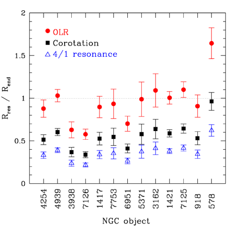
Figure 4: Ratios of resonance positions, $R_{res}$, to spiral endpoints, $R_{end}$. Except in the case of NGC 4254 (M 99), objects are organized by their Hubble type; values of the resonances and spiral endpoints are listed in Table  4. Filled circles: OLR; filled squares: corotation; empty triangles: 4:1 resonance.

5 Expected $Q(rJgi)$ index profiles in a spiral shock scenario.

In this section, we consider in a qualitative way a more realistic situation within the density wave scenario.

The relative density distributions of young and old stars after the shock, as well as non-circular stellar velocities produce changes in the azimuthal light profiles with respect to the idealized case discussed earlier. Also, since we are dealing with different generations of stars, metallicity variations should be considered. In what follows, we discuss each one of these issues at moderate length, and make an estimate of their impact on the disk dynamic parameters derived through the comparison of model and observed $Q$ profiles.

5.1 Post-shock density and velocity distributions.

With the purpose of increasing our understanding of gas dynamics in the presence of spiral density waves, stationary spiral shock patterns have been studied with both semi-analytical approaches (e.g., Roberts, 1969; Gittins & Clarke, 2004) and numerical simulations (e.g., Slyz et al., 2003; Martos et al., 2004; Yáñez et al., 2008). The post-shock density and velocity profiles obtained from such studies show that they depend on many physical parameters. It is reasonable to assume, however, that the newborn stars product of these shocks have densities and velocities that are similar to those of the collapsed gas clouds where they form, at least in the early stages of their evolution, and even if only a few percent of the gas will form stars. Also, it is commonly accepted that dust lanes trace the location of spiral shocks. As newborn stars move away from their birth site, different distances are reached due to accelerated movements. In figure 5 we show the gas velocity parallel to the spiral equipotential curve from the semi-analytical solution of Roberts (1969); this solution corresponds to a radius of 10 kpc; a pattern speed, $\Omega_{p}$, of 12.5 km s^-1 kpc^-1; an arm pitch angle $i=8\fdg 13$; a spiral field strength of 5% that of the axisymmetric field; and a mean gaseous dispersion of 10 km s^-1. The distance is measured relative to the spiral shock location, and the velocity, in the non-inertial frame of reference of the spiral pattern. The variable velocity in an inertial frame of reference goes from 235 to 255 km s^-1. For the time being, we assume that the circular gas velocity is approximately equal to this velocity, and investigate the effects of such variable stellar velocity on the 1-D profiles of the photometric index $Q(rJgi)$.

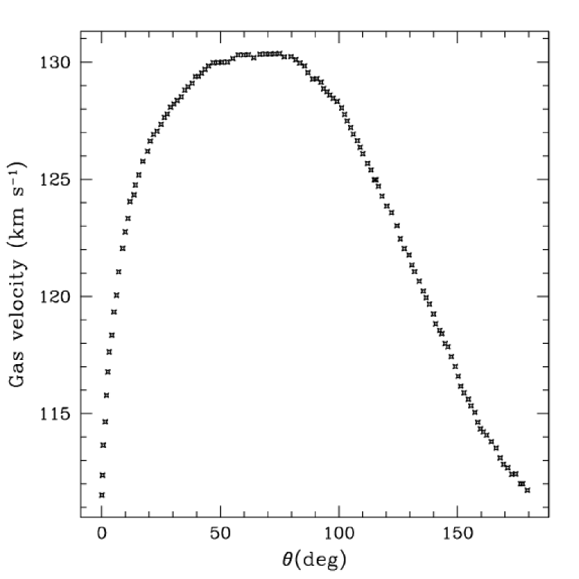
Figure 5: Gas circular velocity vs. angular distance obtained from the solution by Roberts (1969). The distance is measured relative to the spiral shock location, and the velocity, relative to the non-inertial frame of reference of the spiral pattern. We assume that the gas circular velocity is approximately equal to the velocity parallel to the spiral equipotential.

Figure 6 shows theoretical profiles for the $Q(rJgi)$ index, obtained with the variable velocity plotted if Fig. 5. The models have an IMF upper mass limit of 10 $M_{\sun}$, and a constant fraction of young stars of 2% throughout. A comparison with constant velocities of 120 km s^-1 and 240 km s^-1 is also shown.

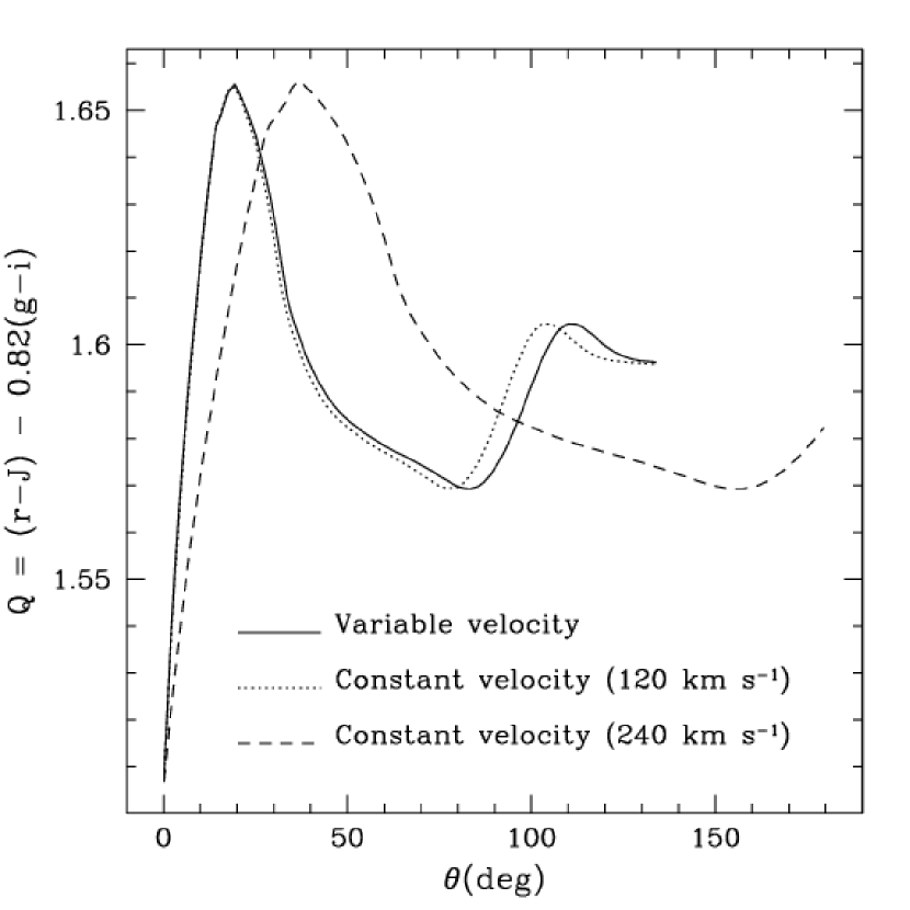
Figure 6: Theoretical profiles for the $Q(rJgi)$ photometric index, CB07 models. Solid line: stars have a variable orbital velocity, as shown in Fig. 5; dotted line: stars have a constant circular velocity of 120 km s^-1; dashed line: stars with a constant orbital velocity of 240 km s^-1.

Next, we investigate the effect of including variable, more realistic, mass fractions of old and young stars. To this end, we use the relative gas density shown in Fig. 7. This density was derived by Roberts (1969), using the same parameters listed above for his velocity solution. We then assume that the fraction of young stars must be 2% at an age of $3\times 10^{7}$ years ($\theta\sim 20\arcdeg$), and propagate this fraction to other locations, supposing that the young stars share the gas density distribution (for example, the young stars fraction would be about 2.5% at an age of $1.5\times 10^{7}$ years or $\theta\sim 10\arcdeg$). As already stated, for the old stars mass fraction we use $\beta_{II}$ = 1 - $\beta_{I}$ (see equation 9). The theoretical $Q$ profiles involving variable stellar velocities, and both variable and constant stellar densities are shown in figures 8 and 9, for IMF upper mass limits of 10 and 100 $M_{\sun}$, respectively.

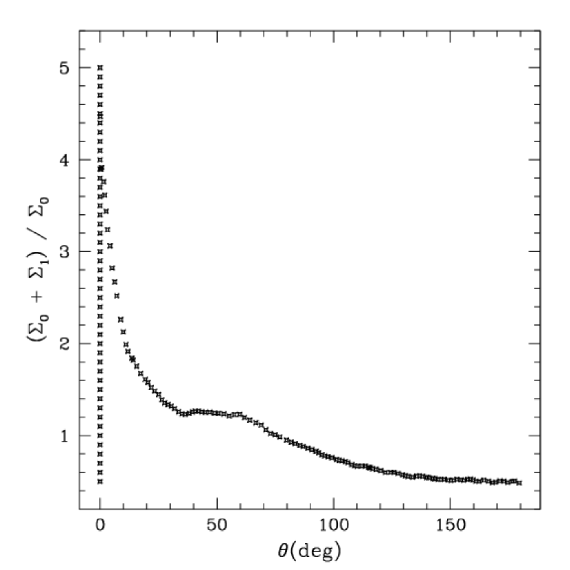
Figure 7: Gas relative density from the shock solution of Roberts (1969). $\Sigma_{0}$ is the unperturbed density in the axisymmetric potential, and $\Sigma_{1}$ is the perturbed density due to the spiral gravitational field. The resulting total gas density is $\Sigma=\Sigma_{0}+\Sigma_{1}$.

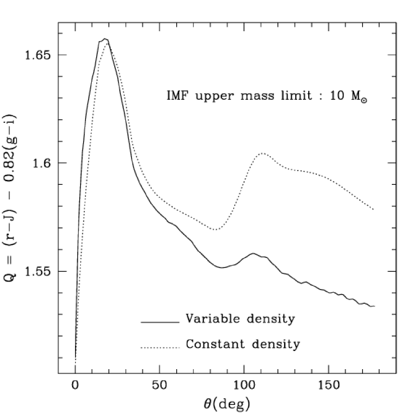
Figure 8: Model profiles for the photometic index $Q(rJgi)$, low IMF upper mass limit. Solid line: variable stellar velocity and density as shown in figures 5 and 7, respectively. Dotted line: variable stellar velocity and constant density (2% of young stars by mass). The IMF lower and upper mass limits are 0.1 and 10 $M_{\sun}$, respectively, for both models.

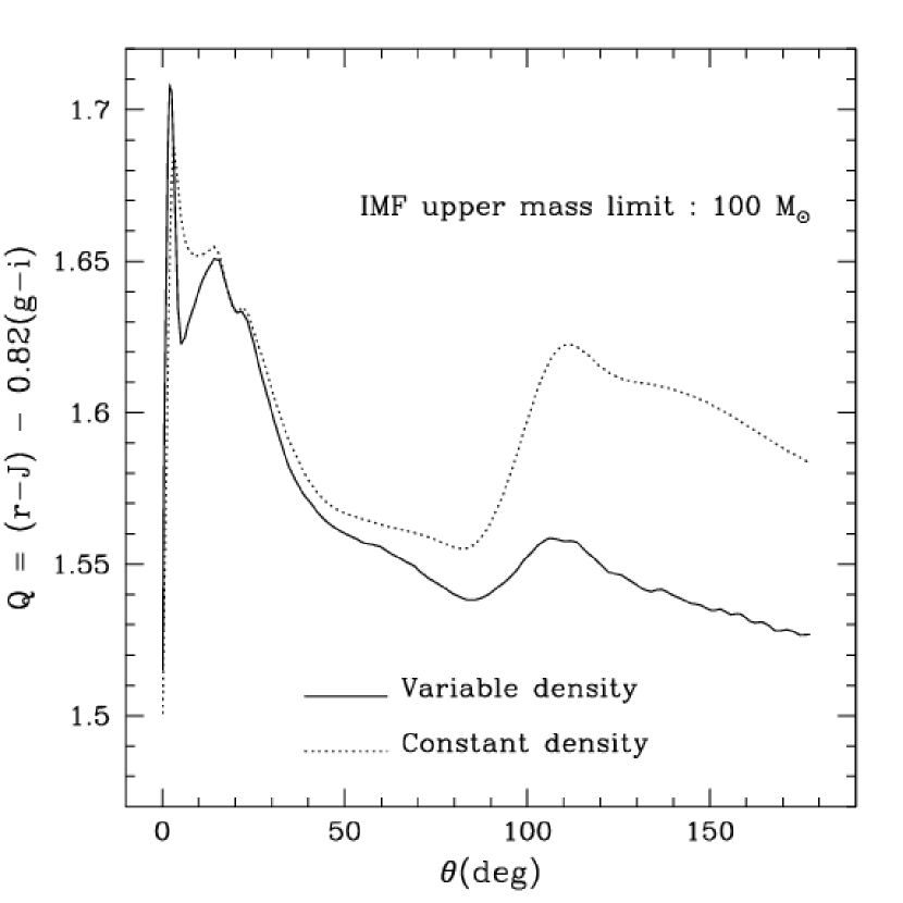
Figure 9: Model profiles for the photometic index $Q(rJgi)$, high IMF upper mass limit. Solid line: variable stellar velocity and variable stellar density; dotted line: variable stellar velocity and constant density. The IMF lower and upper mass limits are 0.1 and 100 $M_{\sun}$, respectively, for both models.

A further possible refinement to the models concerns the relative location of the shock and the potential minimum. According to Gittins & Clarke (2004), the shock location moves to different azimuthal values for tightly wound spirals. At small radii (inside corotation), the shock occurs near the potential minimum; at larger radii, though, the shock weakens and moves upstream towards the potential maximum. In real galaxies, the maximum surface density of old stars and the potential minimum will not coincide exactly (Zhang & Buta, 2007). The gas responds to the potential minimum, while the maximum observed surface density of old stars marks the peak of the density wave. The old stars’ surface density is commonly inferred from observations at 2$\mu$m, although red supergiants may contribute 20% of the flux in this wavelength (Rix & Rieke, 1993). Assuming that the onset of star formation occurs almost immediately after the shock, the resulting total stellar density (i.e., considering both young and old stars) will be affected by the relative positions of each component. In Fig. 10, we show a possible shape for a density wave taken from the $K_{s}$ data of NGC 7125, assuming all the emission comes from an old population with a constant mass-to-light ratio. We try three positions of the density wave peak at, respectively, 10, 15, and 20 degrees away from the shock, with increasing widths. With these density distributions of old stars, and the variable velocity and relative density distributions for young stars discussed previously (the fraction of young stars is taken to be 2% at an age of $3\times 10^{7}$ years, and propagated to other positions following the gas density distribution shown in Fig. 7), we produce once again theoretical profiles for the $Q(rJgi)$ index. These are shown in figures 11 and 12, for IMF upper mass limits of 10 and 100 $M_{\sun}$, respectively. The comparison between the more complex models and those with constant stellar densities and velocities are also shown in this figures, for a fraction of young stars of 2% by mass. From this analysis it is clearly seen that galaxy azimuthal light profiles may suffer deformations depending on the density and velocity distributions of the underlying stars, being the deformation due to density the most important one.

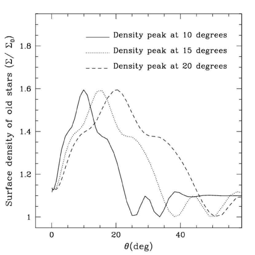
Figure 10: Density profiles of old stars for different locations of the density wave relative to the spiral shock. Solid line: old population density peak at 10$\arcdeg$; dotted line: density peak at 15$\arcdeg$; dashed line: density peak at 20$\arcdeg$. $\Sigma_{0}$ is the unperturbed density in an axisymmetric potential; $\Sigma_{1}$ corresponds to the density wave perturbation; $\Sigma=\Sigma_{0}+\Sigma_{1}$. Angular locations are the same as in previous figures.

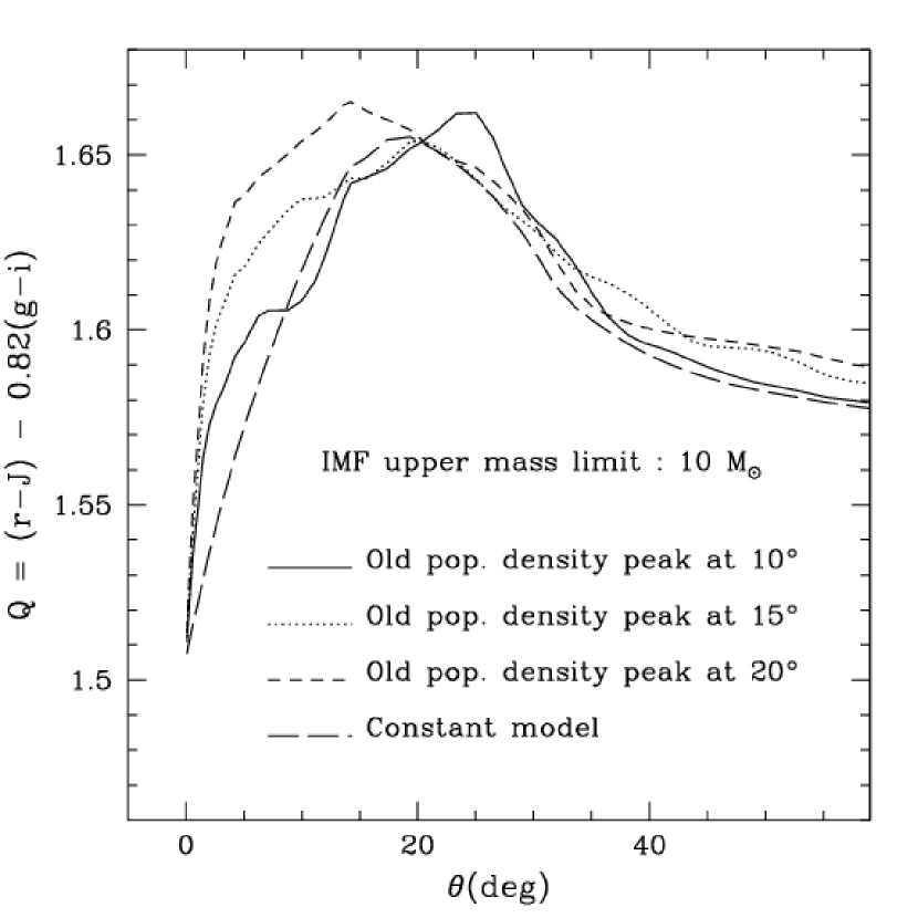
Figure 11: Theoretical $Q$ profiles for variable stellar densities and velocities, in the case of an IMF upper mass limit of 10 $M_{\sun}$. Each model corresponds to a different location of the stellar density wave peak, as shown in Fig. 10. Lines have same meaning as in Fig. 10, except for the long-dashed line: constant stellar density and velocity.

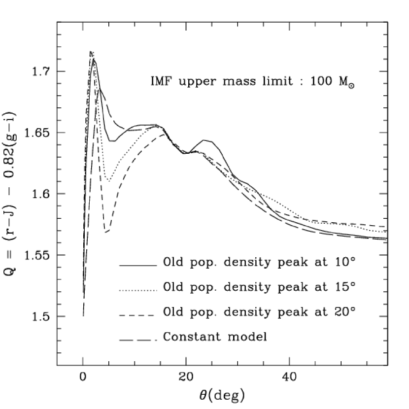
Figure 12: Same as Fig. 11, for an IMF upper mass limit of 100 $M_{\sun}$. The main difference with respect to Fig. 11 is the sharp peak at $\theta\sim 0\arcdeg$.

It is worth noticing that in models with constant stellar density and velocity a degeneracy occurs between IMF upper mass limit and fraction of young stars (GG96), where models with low IMF upper mass limit and higher young star fraction resemble those with high upper mass limit and lower young star fraction (1 %). This degeneracy is shown in Fig. 13. In models with a fraction of young stars that varies with azimuthal position, however, this degeneracy is broken, as is shown in figures 11 and 12. The models with an upper mass limit of 100 $M_{\sun}$ show a peak close to the shock that is absent in those with $M_{upper}$ = 10 $M_{\sun}$, although it is true that the peak might be lost in data with a poor signal-to-noise ratio.

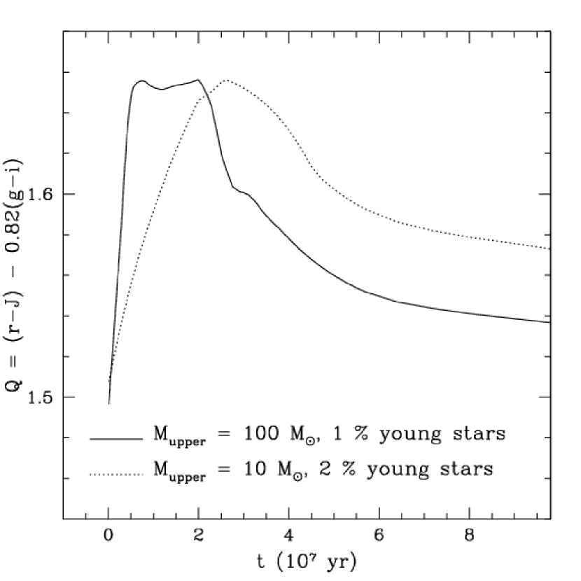
Figure 13: Degeneracy in constant stellar density models between IMF upper mass limit and fraction of young stars. Solid line: $M_{upper}=100M_{\sun}$ and 1% (by mass) of young stars; dotted line: $M_{upper}=10M_{\sun}$ and 2% of young stars. Burst duration is $2\times 10^{7}$ years. The difference in the derived $\Omega_{p}$ from the two models would be $\sim$ 3 km s^-1 kpc^-1.

5.2 Non-circular motions.

The motions of young stars under the assumption of spiral density wave triggering have been studied by, among others, Yuan (1969); Wielen (1973, 1978, 1979); Fernández et al. (2008). Wielen (1979) has emphasized that, in a galaxy with spiral density waves, newly-born stars have not had time to reach dynamical equilibrium with the galaxy potential. Hence, instead of responding to a stationary wave like the old population, young stars migrate out of the arms following complicated, non-circular, orbits. The aforementioned trajectories are not necessarily closed; also, they can run almost parallel to the arms for significant stretches, with the consequence that stars are not seen leaving the arms until they have somewhat aged and at a radius where the dust lane location does not mark the site of star formation; stars might even move to locations upstream of the shock. The color gradients discussed before would overlap with stars drifting back to the arms.

Another consequence in real galaxies is that orbits are no longer vertical lines in the $\theta$ vs. $\ln R$ plane; rather, they are oblique and wavy, as shown in Fig. 14. Given that we have collapsed our data in radius to improve the signal-to-noise ratio, our analysis is insensitive to this effect.

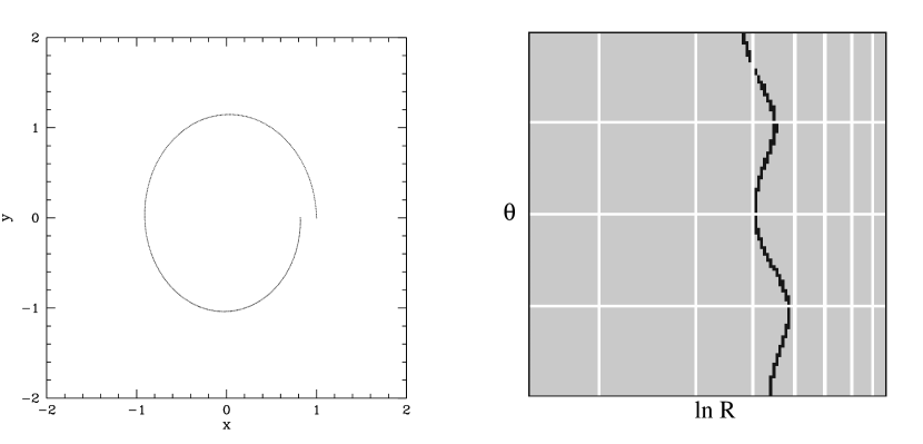
Figure 14: Left: Orbit in cartesian coordinates (arbitrary units). Right: The same orbit in the $\theta$ vs. $\ln R$ plane. Vertical lines represent circles every $\sim 0.3$ arbitray units ($R=\sqrt{x^{2}+y^{2}}$). Horizontal lines are distributed every $90\arcdeg$.

Finally, if molecular clouds suffer the effects of the spiral shock, drift velocities will be smaller and stars will take longer to migrate away from the arms, as shown in Fig. 5 of Wielen (1979); there, lines of equal stellar age are closer together than in his Fig. 4, where clouds and young stars keep their pre-shock velocities.

Qualitatively, these phenomena are akin to the variable stellar velocities and densities considered in § 5.1, and whose impact on the derived density wave parameters is minimal, as briefly discussed in § 5.4. Numerical simulations beyond the scope of this paper would be required to assess their repercussions in a quantitative way.

5.3 The role of metallicity.

The chemical composition of spiral disks has been studied by several authors, mainly through spectroscopic studies of HII regions (Vila-Costas & Edmunds, 1992; Zaritsky, Kennicutt & Huchra, 1994; van Zee et al., 1998; Garnett, 2002). Zaritsky, Kennicutt & Huchra (1994) measured the oxygen abundance, using a photoionization model for calibration, in 39 disk galaxies at the characteristic radius $r=0.4\rho_{0}$, where $\rho_{0}$ is the $B$ = 25 mag arsec^-2 isophotal radius. Their main result for various Hubble types is shown in Fig. 15.

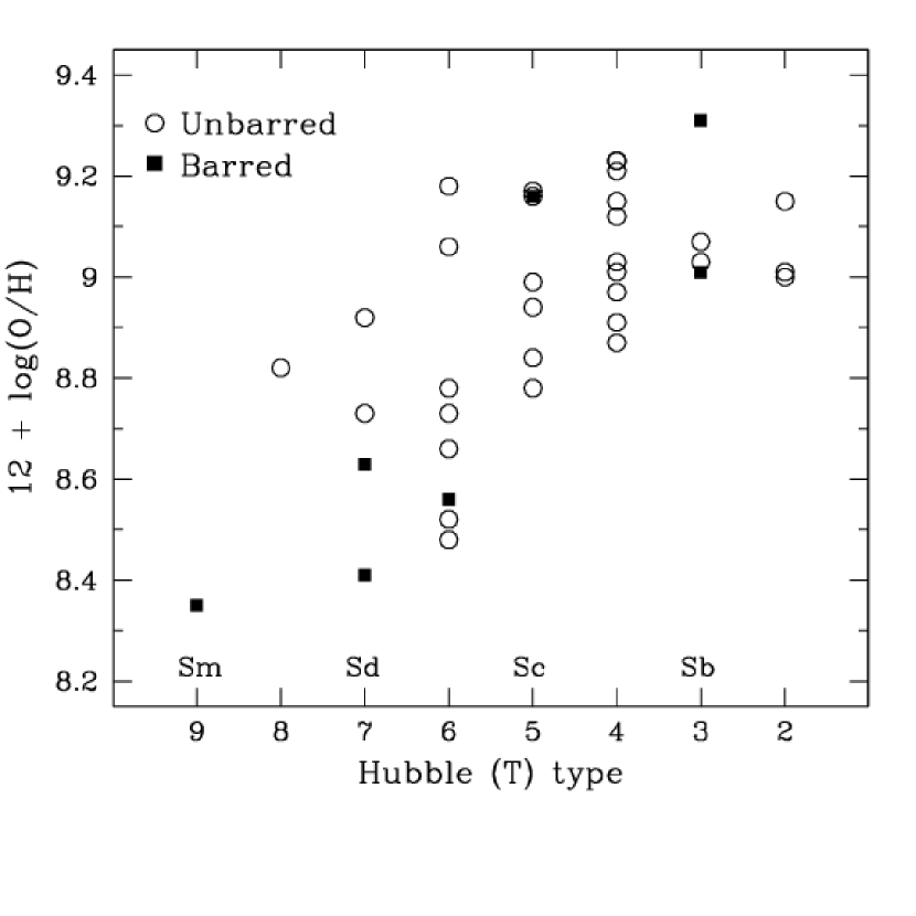
Figure 15: Characteristic abundance vs. Hubble type (T-type as defined by RC2) from Zaritsky, Kennicutt & Huchra (1994). Smaller T-types correspond to earlier type galaxies.

Adopting the usual normalization $X$ + $Y$ + $Z$ = 1, where $X$, $Y$, and $Z$ are, respectively, the abundances per unit mass of hydrogen, helium, and the remaining elements, we have:

$$\frac{Z(O)}{X}=16(O/H),$$ (10)

where $Z(O)/Z$ is the fraction of $Z$ due to oxygen. This fraction varies with metallicity between 41% and 53% in the Local Group of galaxies (Peimbert, 2003). Taking the values $X$ = 0.75 and $Z(O)/Z$ = 0.45, the expression for $Z$ in terms of the oxygen abundance is:

$$\log(Z)\simeq 1.43+\log(O/H).$$ (11)

Assuming that young stars have metallicity values around the ones inferred from abundance ratios, we obtain that $Z$ is in the range $[0.006,0.05]$ for the disk stars in the Zaritsky et al. (1994) sample. In Fig. 16 we show the behavior of the $Q$ index for various combinations of metallicities for the young and old stars, using the CB07 models. In these models the adopted solar metallicity is $Z_{\sun}=0.02$. The duration of the burst is $2\times 10^{7}$ years, both young and old stars have a Salpeter IMF with $M_{lower}=0.1M_{\sun}$ and $M_{upper}=100M_{\sun}$. The fraction of young stars is 2% by mass, and the old stellar background population is $5\times 10^{9}$ years old.

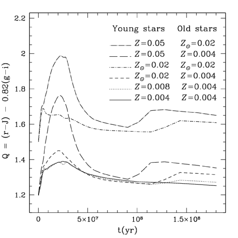
Figure 16: $Q$ index behavior with different combinations of metallicities for the young and old stars. Solid line: $Z_{\rm young}=0.004$, $Z_{\rm old}=0.004$; dotted line: $Z_{\rm young}=0.008$, $Z_{\rm old}=0.004$; dashed line: $Z_{\rm young}=0.02$, $Z_{\rm old}=0.004$; dashed-dotted line: $Z_{\rm young}=0.02$, $Z_{\rm old}=0.02$; long-dashed line: $Z_{\rm young}=0.05$, $Z_{\rm old}=0.004$; long-dashed-dotted line: $Z_{\rm young}=0.05$, $Z_{\rm old}=0.02$.

When young stars have $Z>Z_{\sun}$, $Q$ reaches much higher values than in models where young stars have subsolar metallicities. Models that differ in the metallicities of the young population show different $Q$ values mainly between 1$\times 10^{7}$ and 3$\times 10^{7}$ yr, when the young stars are most prominent; if, on the other hand, the young stars have the same $Z$ but the old populations do not, the models run basically parallel, with a roughly constant offset in the $Q$ values at all ages.

5.4 Simple vs. complex models.

Through the comparison between examples of the more complex models presented and our data, we estimate that ignoring the deformations produced by variable densities, variable velocities, and different metallicities (see § 5.1, § 5.2 and § 5.3) would translate into a maximum error of approximately $\pm$1 km s^-1 kpc^-1 in $\Omega_{p}$ (see also the Appendix). This quantity is well within the random errors computed for $\Omega_{p}$ shown in Table 4.

The small size of this error might signal a sort of selection bias: if non-linear effects were very important, it would be unlikely to find a gradient. On the other hand, remarkably, we have been able to detect gradients in an unprecedented 10 out of 13 galaxies. Not only have we quadrupled the historic number of detections, but we have found gradients in more than 75% of the subsample analyzed in this paper, that does not even comprise (with the exception of M 99) the “$Q$ effect” galaxies, i.e., the objects with the strongest features. This means that non-linear effects that would deform all gradients beyond recognition might not be too significant in galaxies with spiral density waves. When GG96 found the gradient in M 99, an obvious question that arose was whether NGC 4254 was an exception or if an adequate technique to search for the gradients had been finally devised. The present work answers that question unambiguously.

Furthermore, the comparison of the gradients with the simplest of models yields orbital resonance positions that match the observed spiral endpoints. These results agree with the predictions of density wave theory, and establish a strong link between disk dynamics and large scale star formation, as we argue below.

6 Discussion and conclusions.

If star formation is related to disk dynamics then, according to theory, the $R_{res}/R_{end}$ ratio must be close to one, for either the 4:1 resonance, the corotation radius, or the OLR. Contopoulos & Grosbøl (1986), based on orbital calculations, determined that the spiral pattern of strong spirals must extend to the 4:1 resonance. Patsis, Contopoulos & Grosbøl (1991) defined strong spirals as those with large pitch angles (i.e., Sb and Sc galaxies, that are not tightly wound); their theory is considered “non linear”. Conversely, the “linear” theory of spiral density waves concerns itself with tightly wound spirals and has concluded that the arms of some normal (nonbarred) spirals reach corotation (Lin, 1970) and are stationary, while those of others grow to the OLR (Mark, 1976; Lin & Lau, 1979; Toomre, 1981). In the Contopoulos & Grosbøl (1986) treatment, the “linear” theory is recovered when spiral arms are not strong (as in Sa galaxies).

In Fig. 4, we can see that most spirals in our sample extend to the OLR and one of them (NGC 578) reaches corotation. The mean of the ratio $R_{OLR}/R_{end}$, for all 13 points, is 0.95$\pm$0.03. The reduced $\chi^{2}/n$ of this result is 7.12; the probability of this result being due to chance for 13 degrees of freedom is less than 1 out of 10,000. If we remove the points corresponding to NGC 3938, NGC 7126, NGC 6951, and NGC 578, $R_{OLR}/R_{end}=0.98\pm 0.04$, with a reduced $\chi^{2}/n$ = 0.48, for $n=9$. This last result may indicate that some of our errors are overestimated. It is interesting to note that none of our objects is an Sa (weak spiral) galaxy. From this we may conclude that the “linear” result for the extent of spiral patterns applies to strong spirals too!

On the other hand, for most objects the spiral begins at the location of the ILR, as expected. For the analysis presented here, though, the location of this resonance should be taken with care, since we are employing flat rotation curves, even at small radii. When using real rotation curves, the positions of the ILRs for our sample may vary. The possibility also exists that there is no ILR in some objects.

In some regions, the downstream values of the $Q$ index are lower than the models. This is the case for NGC 4939 A, NGC 3162 B, NGC 1421 A, NGC 1421 C, NGC 7125 A, NGC 7125 C, NGC 578 A, and NGC 578 B. For the present analysis we have assumed that every star-forming region maintains its previous circular motion after the spiral shock. As already stated, in real galaxies the situation is different: variations in the velocity vector are present due to the shock itself and the resulting loss of angular momentum (Yuan & Grosbøl, 1981; Fernández et al., 2008). This effect could explain the “downstream fall” of the gradients. Metallicity is another factor that can play a significant part: a lower metallicity of the older stars may produce a steep drop of the gradients (see § 5.3).

We have shown that azimuthal color gradients are common in spiral arms of disk galaxies. Even inverse color gradients have been found in the arms of NGC 1421, NGC 4939, and NGC 7125. The observed picture is, of course, not as clean as originally envisioned, for several reasons. Dust and HII regions may mask the gradients (GG96); indeed, all the detected gradients have been satisfactorily fitted with models where $M_{upper}$ = 10 $M_{\odot}$. Other star formation mechanisms, like self-propagating star formation, may take place simultaneously with density wave triggering in spiral arms and disks in general. Likewise, there may be substructure formation, as a result of non-linear and chaotic effects associated to the wave phenomenon itself (Chakrabarti et al., 2003; Dobbs & Bonnell, 2006; Kim & Ostriker, 2006; Shetty & Ostriker, 2006). In the future, three aspects can be improved when carrying out this type of study. (1) A better determination of the inclination angle of the galaxy, and of the rotation curve at different radii; this will reduce the uncertainty in $\Omega_{p}$. (2) The inclusion in the models of the variable density distributions of young and old stars, as well as of the stellar velocity changes near the spiral shocks. This will account for non-circular motions near the spiral shocks and for the higher order terms in equation 2. Numerical simulations or semi-analytical treatments may be needed, particularly for the young stars; also, the contribution of red supergiants to the observed $K$-band surface brightness should be considered when modeling the distribution of old stars. (3) Spectroscopic studies could be very helpful as diagnostics of the population properties, particularly of the metallicity along the gradients.

According to the dynamic parameters derived from our analysis, spiral arms mostly extend to the OLR and sometimes to the corotation radius. Ten of thirteen objects (77%) support this conclusion. Similar results have been obtained by other authors as well (e.g., Elmegreen et al., 1992; Zhang & Buta, 2007). In view of the consistency between the pattern speeds and resonance positions determined from the azimuthal stellar gradients, and the predictions of density wave theory, we conclude that disk dynamics do play an important role in large scale star formation in some spiral galaxies.

Appendix A Pattern speed and corotation radius error calculation.

In principle, the three contributors to the random error in the pattern speed, $\sigma_{\Omega_{p}}$ (km s^-1 kpc^-1), are the uncertainties in: the inclination angle, $\sigma_{\alpha}$; the rotation velocity, $\sigma_{v_{max}}$; and the distance to the galaxy, $\sigma_{D}$.

In order to compute $\sigma_{\Omega_{p}}$ from equation 6, and hence the uncertainty in the resonance positions, we replace $R_{mean}$, $v_{rot}$, and $d$ with their corresponding expressions in terms of independent variables. We obtain:

$$\Omega_{p}=\frac{k_{1}v_{max}}{rD(\sin\alpha)}-\frac{k_{2}}{t}\cos^{-1}\left(\frac{\frac{x_{1}x_{2}}{\cos^{2}\alpha}+y_{1}y_{2}}{r^{2}}\right),$$ (A1)

$$r=\frac{\sqrt{\frac{x^{2}_{1}}{\cos^{2}\alpha}+y_{1}^{2}}+\sqrt{\frac{x^{2}_{2}}{\cos^{2}\alpha}+y_{2}^{2}}}{2},$$ (A2)

where constant $k_{1}=\frac{648000}{p_{s}\pi}$ (pixels), $p_{s}$ is the adopted plate scale in arsec pixel^-1, constant $k_{2}=9.766\times 10^{8}$ (yr km s^-1 kpc^-1), $r$ is the mean deprojected radius of the region in pixels; $v_{max}$ is the maximum rotation velocity in km s^-1; $(x_{1},y_{1})$ and $(x_{2},y_{2})$ are the cartesian coordinates (in pixels) of the extremes of the curved line segment corresponding to the studied region in the non-deprojected image (the origin is located at the center of the object and the galaxy major axis runs along the y coordinate); $D$ is the distance to the object in kpc; $\alpha$ is the inclination angle used to deproject the image; and $t$ is the stellar model age in years.

The corotation radius, $R_{\rm CR}$ (kpc), is:

$$R_{\rm CR}=\frac{v_{max}}{(\sin\alpha)\Omega_{p}}.$$ (A3)

The expressions for each contributor to the error calculation are:

$$\Delta\Omega_{p}[\alpha]=\Omega_{p}(\alpha+\sigma_{\alpha},v_{max},D,t)-\Omega_{p}(\alpha,v_{max},D,t)$$ (A4)

$$\Delta\Omega_{p}[v_{max}]=\Omega_{p}(\alpha,v_{max}+\sigma_{v_{max}},D,t)-\Omega_{p}(\alpha,v_{max},D,t)$$ (A5)

$$\Delta\Omega_{p}[D]=\Omega_{p}(\alpha,v_{max},D+\sigma_{D},t)-\Omega_{p}(\alpha,v_{max},D,t)$$ (A6)

$$\sigma_{\Omega_{p}}=\sqrt{(\Delta\Omega_{p}[\alpha])^{2}+(\Delta\Omega_{p}[v_{max}])^{2}+(\Delta\Omega_{p}[D])^{2}}.$$ (A7)

Values for $\pm\sigma$ were calculated, and the absolute $\Delta\Omega_{p}$ values were averaged. Similar expressions hold for $\sigma_{R_{\rm CR}}$. Figure 17 shows the $\Delta\Omega_{p}$ and $\Delta R_{\rm CR}$ absolute average values for each region listed in Table 4. The systematic error due to the choice of stellar population model was estimated by comparing the $\Omega_{p}$ values derived with the simple models of § 3, on the one hand, with examples of the more complex models discussed in § 5.4, on the other.

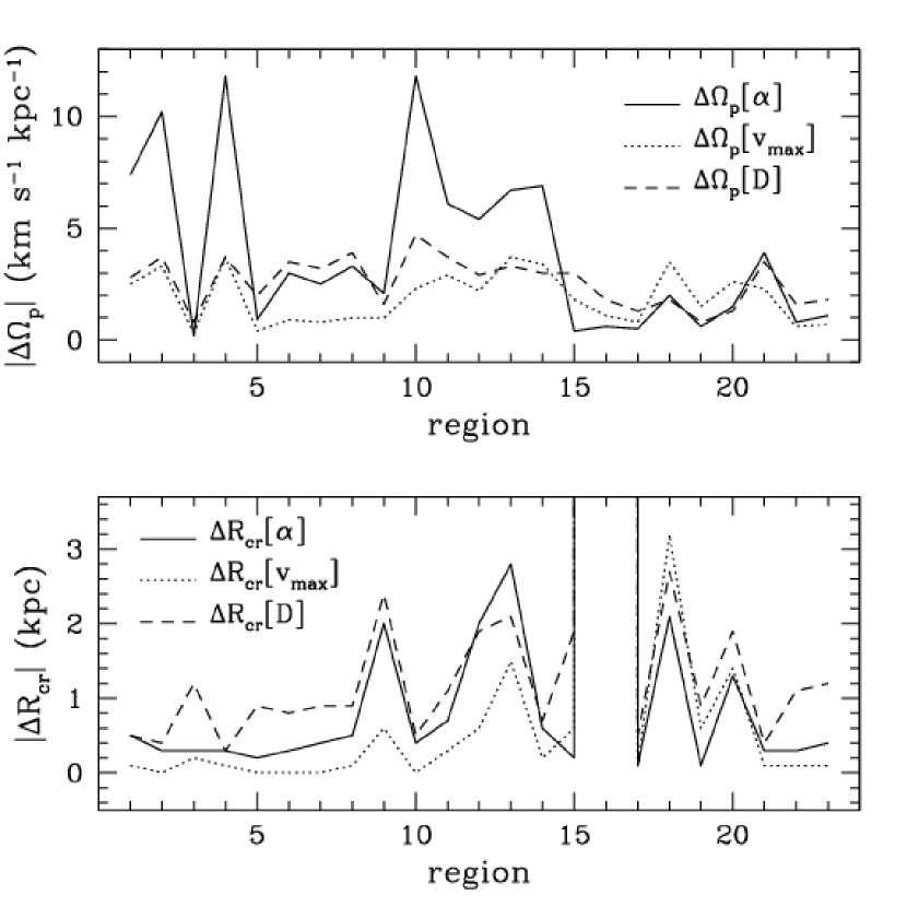
Figure 17: Absolute $\Delta\Omega_{p}$ and $\Delta R_{\rm CR}$ average values for galaxy regions. Regions are identified by their numbers in Table 4. Solid line: contribution from inclination angle, $\alpha$; dotted line: contribution from rotation velocity, $v_{max}$; dashed line: contribution from distance to the galaxy, $D$. The measurements are shown as continuous lines for easiness of reading; in reality, they are discrete points.

Figure 20: Region NGC 4939 A. In order to fit the model to the data we assume the gradient is inverse, occurring beyond corotation. This can also be seen from the fact that time evolution (top axis in panel $c$) and rotation have opposite directions.

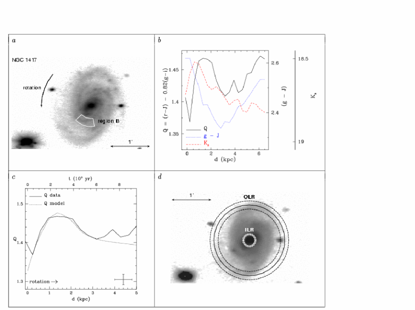
Figure 25: Region NGC 1417 B. Panel $d$: $J$-band deprojected mosaic of spiral galaxy NGC 1417.

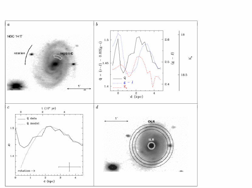
Figure 26: Region NGC 1417 C. Panel $d$: $J$-band deprojected mosaic of spiral galaxy NGC 1417.

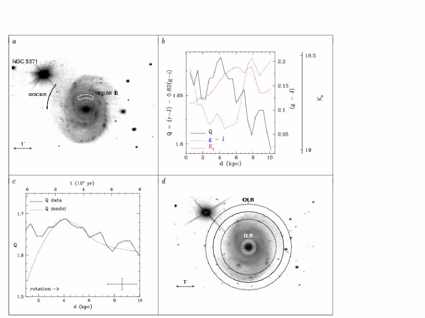
Figure 30: Region NGC 5371 B.

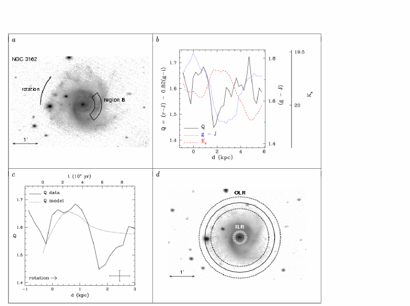
Figure 32: Region NGC 3162 B. Panel $d$: $J$-band deprojected mosaic of spiral galaxy NGC 3162.

Figure 33: Region NGC 1421 A.

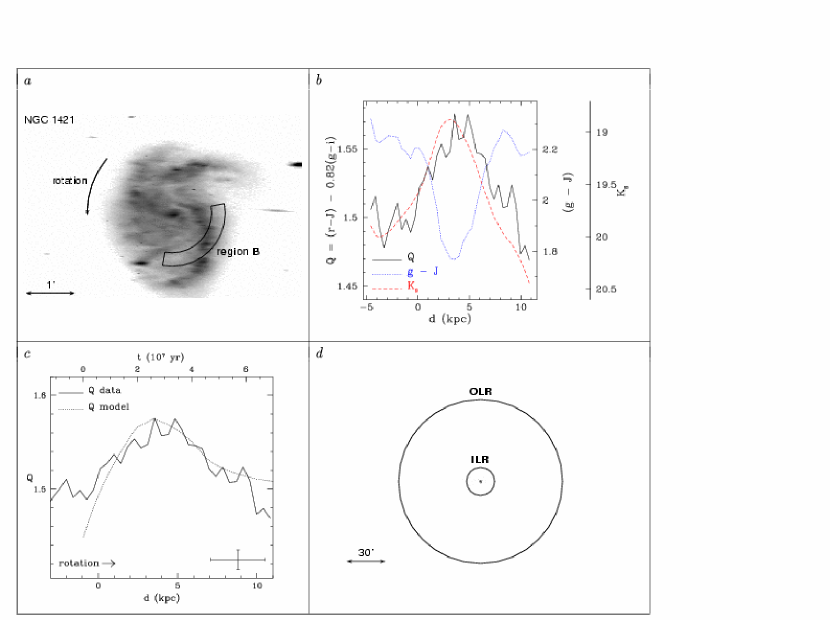
Figure 34: Region NGC 1421 B. Panel $d$, solid line circle: location of the ILR and the OLR, as obtained from the comparison between data and SPS model shown in panel $c$. The errors for the resonance positions are much greater than the computed resonance radii themselves (see Fig. 17). This is due to the fact that region B lies right on the corotation position obtained from regions A & C.

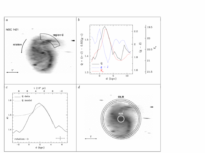
Figure 35: Region NGC 1421 C.

Figure 37: Region NGC 7125 B. Panel $d$: $J$-band deprojected mosaic of spiral galaxy NGC 7125.

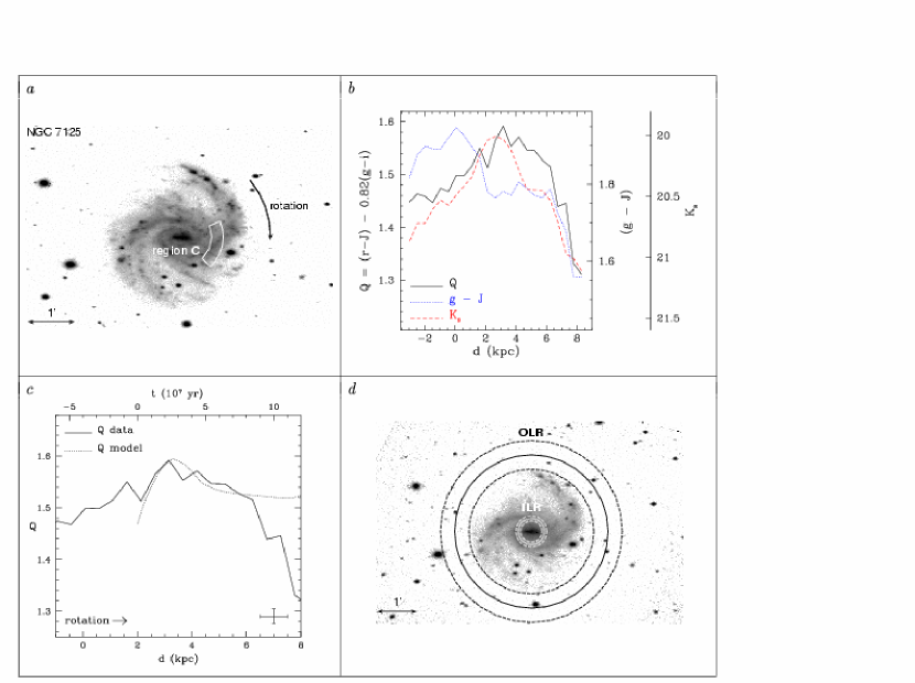
Figure 38: Region NGC 7125 C. Panel $d$: $J$-band deprojected mosaic of spiral galaxy NGC 7125.

Figure 41: Region NGC 578 B. Panel $d$, $K_{s}$-band deprojected mosaic of spiral galaxy NGC 578. solid line circles: location of the ILR and corotation radius, as obtained from the comparison between data and SPS model shown in panel $c$.

References

- Allen (1996) Allen, R. J. 1996, New Extragalactic Perspectives in the New South Africa, 209, 50
- Ballesteros-Paredes & Hartmann (2007) Ballesteros-Paredes, J., Hartmann, L. 2007, Rev. Mexicana Astron. Astrofis., 43, 123
- Ballesteros-Paredes, Hartmann & Vázquez-Semadeni (1999) Ballesteros-Paredes, J., Hartmann, L., Vázquez-Semadeni, E. 1999, ApJ, 527, 285
- Bertin et al. (1989a) Bertin, G., Lin, C. C., Lowe, S. A., Thurstans, R. P. 1989a, ApJ, 338, 78
- Bertin et al. (1989b) Bertin, G., Lin, C. C., Lowe, S. A., Thurstans, R. P. 1989b, ApJ, 338, 104
- Binney & Merrifield (1998) Binney, J., & Merrifield, M. 1998, Galactic Astronomy (Princeton: Princeton Univ. Press)
- Block & Wainscoat (1991) Block, D. L., & Wainscoat, R. J. 1991, Nature, 353, 48
- Bruzual & Charlot (1993) Bruzual, A. G., Charlot, S. 1993, ApJ, 405, 538
- Bruzual & Charlot (2003) Bruzual, G., Charlot, S. 2003, MNRAS, 344, 1000
- Bruzual, Magris & Calvet (1988) Bruzual, A. G., Magris, G., Calvet, N. 1988, ApJ, 333, 673
- Burningham et al. (2005) Burningham, B., Naylor, T., Littlefair, S. P., Jeffries, R. D. 2005 ,MNRAS, 363, 1389
- Carigi & Peimbert (2008) Carigi, L., & Peimbert, M. 2008, Rev. Mexicana Astron. Astrofis., 44, 341
- Cepa & Beckman (1990) Cepa, J., Beckman, J. E. 1990, ApJ, 349, 497
- Chakrabarti et al. (2003) Chakrabarti, S., Laughlin, G., Shu , F. H. 2003, ApJ, 596, 220
- Charlot & Fall (2000) Charlot, S., & Fall, S. M. 2000, ApJ, 539, 718
- Contopoulos & Grosbøl (1986) Contopoulos, G., & Grosbøl, P. 1986, A&A, 155, 11
- del Río & Cepa (1998) del Río, M. S., & Cepa, J. 1998, A&A, 340, 1
- de Vaucouleurs (1959) de Vaucouleurs, G. 1959, Handb. Phys., 53, 275
- de Vaucouleurs et al. (1976) de Vaucouleurs, G., de Vaucouleurs, A., & Corwin, H. G. 1976, Second reference catalogue of bright galaxies, Austin: University of Texas Press
- de Vaucouleurs et al. (1991) de Vaucouleurs, G., de Vaucouleurs, A., Corwin, H. G., Jr., Buta, R. J., Paturel, G., & Fouque, P. 1991, Volume 1-3, XII, 2069 pp. 7 figs.. Springer-Verlag Berlin Heidelberg New York (RC3)
- Dobbs & Bonnell (2006) Dobbs, C. L., Bonnell, I. A. 2006, MNRAS, 367, 873
- Doom et al. (1985) Doom, C., de Greve, J. P., de Loore, C. 1985, ApJ, 290, 185
- Donner & Thomasson (1994) Donner, K. J., & Thomasson, M. 1994, A&A, 290, 785
- Efremov (1985) Efremov, Y. N. 1985, Soviet Astron. Lett., 11, 69
- Elmegreen & Elmegreen (1983a) Elmegreen, B. G., & Elmegreen, D. M. 1983a, MNRAS, 203, 31
- Elmegreen & Elmegreen (1983b) Elmegreen, B. G., & Elmegreen, D. M. 1983b, ApJ, 267, 31
- Elmegreen & Elmegreen (1986) Elmegreen, B. G., & Elmegreen, D. M. 1986, ApJ, 311, 554
- Elmegreen et al. (1992) Elmegreen, B. G., Elmegreen, D. M., Montenegro, L. 1992, ApJS, 79, 37
- Elmegreen & Lada (1977) Elmegreen, B. G., Lada, C. J. 1977, ApJ, 214, 725
- Eminian et al. (2008) Eminian, C., Kauffmann, G., Charlot, S., Wild, V., Bruzual, G., Rettura, A., & Loveday, J. 2008, MNRAS, 384, 930
- Fernández et al. (2008) Fernández, D., Figueras, F., Torra, J. 2008, A&A, 480, 735
- Garnett (2002) Garnett, D. R. 2002, ApJ, 581, 1019
- Gittins & Clarke (2004) Gittins, D. M., Clarke, C. J. 2004, MNRAS, 349, 909
- González & Graham (1996) González, R. A., & Graham, J. R. 1996, ApJ, 460, 651 (GG96)
- Hawarden et al. (2001) Hawarden, T. G., Leggett, S. K., Letawsky, M. B., Ballantyne, D. R., Casali, M. M. 2001, MNRAS, 325, 563
- Hayes (1970) Hayes, D. S. 1970, ApJ, 159, 165
- Hamuy et al. (1994) Hamuy, M., Suntzeff, N. B., Heathcote, S. R., Walker, A. R., Gigoux, P., Phillips, M. M. 1994 PASP, 106, 566
- Hamuy et al. (1992) Hamuy, M., Walker, A. R., Suntzeff, N. B., Gigoux, P., Heathcote, S. R., Phillips, M. M. 1992, PASP, 104, 533
- Hodge et al. (1990) Hodge, P.,Jaderlund, E., & Meakes, M. 1990, PASP, 102, 1263
- Indebetouw et al. (2008) Indebetouw, R., et al. 2008, AJ, 136, 1442
- Iye et al. (1982) Iye, M., Okamura, S., Hamabe, M., & Watanabe, M. 1982, ApJ, 256, 103
- Kim & Ostriker (2006) Kim, W.-T., Ostriker, E. C. 2006, ApJ, 646, 213
- Kuchinski et al. (1998) Kuchinski, L. E., Terndrup, D. M., Gordon, K. D., Witt, A. N. 1998, AJ, 115, 1438
- Lauberts (1982) Lauberts, A. 1982, Garching: European Southern Observatory (ESO).
- Lin (1970) Lin, C. C. 1970, in IAU Symp. 38, The Spiral Structure of Our Galaxy, ed. W. Becker & G. I. Contopoulos (Dordrecht: Reidel), 377
- Lin & Lau (1979) Lin, C. C., & Lau, Y. Y. 1979, Stud. Appl. Math., 60, 97
- Lin & Shu (1964) Lin, C. C., & Shu, F. H. 1964, ApJ, 140, 646
- Lindblad (1963) Lindblad, B. 1963, Stockholms Obs. Ann., 22, 5
- Marigo & Girardi (2007) Marigo, P., & Girardi, L. 2007, A&A, 469, 239
- Martos et al. (2004) Martos, M., Hernandez, X., Yáñez, M., Moreno, E., Pichardo, B. 2004, MNRAS, 350, 47
- Mark (1976) Mark, J. W. K. 1976, ApJ, 205, 363
- Massey & Gronwall (1990) Massey, P., Gronwall, C. 1990, ApJ, 358, 344
- Massey et al. (1989) Massey, P., Silkey, M., Garmany, C. D., Degioia-Eastwood, K. 1989, AJ, 97, 107
- Massey et al. (1988) Massey, P., Strobel, K,, Barnes, J. V., Anderson, E. 1988, ApJ, 328, 315
- Mathewson et al. (1972) Mathewson, D. S., Van Der Kruit, P. C., & Brouw, W. N. 1972, A&A, 17, 468
- Mei et al. (2007) Mei, S., Blakeslee, J. P., Côté, P., Tonry, J. L., West, M. J., Ferrarese, L., Jordán, A., Peng, E. W., Anthony, A., Merritt, D. 2007, ApJ, 655, 144
- Morgan et al. (1952) Morgan, W. W., Sharpless, S., & Osterbrock, D. 1952, AJ, 57, 3
- Mould et al. (2000) Mould, J. R. et al. 2000, ApJ, 529, 786
- Mouschovias et al. (2006) Mouschovias, T. Ch., Tassis, K., Kunz, M. W. 2006 ApJ, 646, 1043
- Nilson (1973) Nilson, P. 1973, Uppsala General Catalogue of Galaxies, Acta Universitatis Upsalienis, Nova Regiae Societatis Upsaliensis.
- Oke & Gunn (1983) Oke, J. B., Gunn, J. E. 1983, ApJ, 266, 713O
- Patsis, Contopoulos & Grosbøl (1991) Patsis, P. A., Contopoulos, G., Grosbøl, P. 1991 A&A, 243, 373
- Paturel et al. (2000) Paturel, G., Fang, Y., Petit, C., Garnier, R., Rousseau, J. 2000 , A&AS, 146, 19
- Paturel et al. (2003) Paturel, G., Theureau, G., Bottinelli, L., Gouguenheim, L., Coudreau-Durand, N., Hallet, N., Petit, C. 2003, A&A, 412, 57
- Peimbert (2003) Peimbert, A. 2003, ApJ, 584, 735
- Peletier et al. (1995) Peletier, R. F., Valentijn, E. A., Moorwood, A. F. M., Freudling, W., Knapen, J. H., Beckman, J. E. 1995, A&A, 300, L1
- Persson et al. (1998) Persson, S. E., Murphy, D. C., Krzeminski, W., Roth, M., & Rieke, M. J. 1998, AJ, 116, 2475
- Phookun et al. (1993) Phookun, B., Vogel, S. N., & Mundy, L. G. 1993, ApJ, 418, 113
- Puerari & Dottori (1997) Puerari, I., & Dottori, H. 1997, ApJ, 476, L73
- Rieke & Lebofsky (1985) Rieke, G. H., Lebofsky, M. J. 1985, ApJ, 288, 618
- Rix & Rieke (1993) Rix, H.W., & Rieke, M. J. 1993, ApJ, 418, 123
- Roberts (1969) Roberts, W. W. 1969, ApJ, 158, 123
- Ryder & Dopita (1994) Ryder, S. D., & Dopita, M. A. 1994, ApJ, 430, 142
- Schinnerer et al. (2004) Schinnerer, E., Weiss, A., Scoville, N. Z., & Aalto, S. 2004, BAAS, 36, 812
- Schneider et al. (1983) Schneider, D. P., Gunn, J. E., & Hoessel, J. G. 1983, ApJ, 264, 337
- Seigar & James (2002) Seigar, M. S., & James, P. A. 2002, MNRAS, 337, 1113
- Shetty & Ostriker (2006) Shetty, R., Ostriker, E. C. 2006, ApJ, 647, 997
- Shu (1997) Shu, F. H. 1997, Proceedings of the 21st Century Chinese Astronomy Conference, 21
- Shu, Adams & Lizano (1987) Shu, F. H., Adams, F. C., Lizano, S, 1987, ARA&A, 25, 23
- Shu et al. (1972) Shu, F. H., Milione, V., Gebel, W., Yuan, C., Goldsmith, D. W., & Roberts, W. W. 1972, 173, 557
- Schweizer (1976) Schweizer, F. 1976, ApJS, 31, 313
- Sitnik (1989) Sitnik, T. G. 1989, Soviet Astron. Lett., 15, 388
- Skrutskie et al. (1997) Skrutskie, M. F. et al. 1997, ASSL Vol. 210: The Impact of Large Scale Near–IR Sky Surveys, 25
- Skrutskie et al. (2006) Skrutskie, M. F. et al. 2006, AJ, 131, 1163
- Slyz et al. (2003) Slyz, A. D., Kranz, T., Rix, H.-W. 2003, MNRAS, 346, 1162
- Stone (1977) Stone, R.P.S. 1977, ApJ, 218, 767
- Talbot et al. (1979) Talbot, R. J. Jr., Jensen, E. B., & Dufour, R. J. 1979, ApJ, 229, 91
- Thomasson et al. (1990) Thomasson, M., Elmegreen, B. G., Donner, K. J., & Sundelius, B. 1990, ApJ, 356, L9
- Thuan & Gunn (1976) Thuan, T. X., Gunn, J. E. 1976, PASP, 88, 543
- Tody (1986) Tody, D. 1986, “The IRAF Data Reduction and Analysis System” in Proc. SPIE Instrumentation in Astronomy VI, ed. D.L. Crawford, 627, 733
- Tody (1993) Tody, D. 1993, “IRAF in the Nineties” in Astronomical Data Analysis Software and Systems II, A.S.P. Conference Ser., Vol 52, eds. R.J. Hanisch, R.J.V. Brissenden, & J. Barnes, 173.
- Toomre (1977) Toomre, A. 1977, ARA&A, 15, 437
- Toomre (1981) Toomre, A. 1981, In: The structure and evolution of normal galaxies, Proceedings of the Advanced Study Institute, (Cambridge: Cambridge Univ. Press), 111
- van Zee et al. (1998) van Zee, L., Salzer, J. J., Haynes, M. P., O’Donoghue, A. A., & Balonek, T. J. 1998, AJ, 116, 2805
- Vila-Costas & Edmunds (1992) Vila-Costas, M. B., & Edmunds, M. G. 1992, MNRAS, 259, 121
- Visser (1980) Visser, H. C. D. 1980, A&A, 88, 159
- Vogel (1988) Vogel, S. N., Kulkarni, S. R., Scoville, N. Z. 1988, Nature, 334, 402
- Wade et al. (1979) Wade, R. A., Hoessel, J. G., Elias, J. H., Huchra, J. P. 1979, PASP, 91, 35
- Wainscoat & Cowie (1992) Wainscoat, R. J., & Cowie, L. L. 1992, AJ, 103, 332
- Wielen (1973) Wielen, R. 1973, A&A, 25, 285
- Wielen (1978) Wielen, R. 1978, Structure and Properties of Nearby Galaxies, 77, 93
- Wielen (1979) Wielen, R. 1979, The Large-Scale Characteristics of the Galaxy, 84, 133
- Witt et al. (1992) Witt, A. N., Thronson, H. A., Jr., Capuano, J. M., Jr. 1992, ApJ, 393, 611
- Xilouris et al. (1999) Xilouris, E. M., Byun, Y. I., Kylafis, N. D., Paleologou, E. V., Papamastorakis, J. 1999, A&A, 344, 868
- Yáñez et al. (2008) Yáñez, M. A., Norman, M. L., Martos, M. A., Hayes, J. C. 2008, ApJ, 672, 207
- Yuan (1969) Yuan, C. 1969, ApJ, 158, 889
- Yuan & Grosbøl (1981) Yuan, C., Grosbøl, P. 1981, ApJ, 243, 432
- Zaritsky, Kennicutt & Huchra (1994) Zaritsky, D., Kennicutt, R. C. Jr., Huchra, J. P. 1994, ApJ, 420, 87
- Zhang (1998) Zhang, X. 1998, ApJ, 499, 93
- Zhang & Buta (2007) Zhang, X., & Buta, R. J. 2007, AJ, 133, 2584
- Zwicky (1955) Zwicky, F. 1955, PASP, 67, 232