Two Loop $\boldsymbol{R}$-Symmetry Breaking

Abstract:

We analyze two loop quantum corrections for pseudomoduli in O’Raifeartaigh like models. We argue that $R$-symmetry can be spontaneously broken at two loop in non supersymmetric vacua. We provide a basic example with this property. We discuss on phenomenological applications.

1 Introduction

In the last years a lot of effort has been devoted to the study of supersymmetry breaking in metastable vacua. The starting point has been to understand [1] that metastable and dynamical supersymmetry breaking is a generic phenomenon in $\mathcal{N}=1$ gauge theories [1, 2, 3]. Subsequently these classes of models have been studied in phenomenological settings, where they have been considered as hidden sectors in gauge mediation scenarios [4, 5].

In this framework $R$-symmetry breaking ([6]-[8]) plays an important role. In this note we propose a mechanism for spontaneous $R$-symmetry breaking in supersymmetry breaking vacua through two loop effects.

In the next section we review some aspects about $R$-symmetry breaking in model building. In section 2 we survey a class of models and the corresponding two loop effective potential. In section 3 we present the basic model of metastable supersymmetry breaking with two loop $R$-symmetry breaking. In section 4 we conclude and comment. In the Appendix A we give the details of the two loop computation and in the Appendix B we embed our model in a quiver gauge theory.

1.1 $R$-symmetry breaking

Soft supersymmetry breaking [9] in the MSSM is induced by a mediation mechanism. This is necessary since the supertrace theorem [10]

$$\text{STr}\mathcal{M}^{2}=\sum_{J}(-1)^{2J}(2J+1)M_{J}^{2}$$ (1)

constraints at tree level some masses of the superpartners to be lower than the masses of the ordinary particles.

In the case of gauge mediation, supersymmetry is broken in a secluded sector, and then transmitted to the visible sector (the MSSM). The breaking in the hidden sector can be spontaneous or dynamical, even in metastable vacua. There is a messenger sector coupled with the secluded sector and charged under the MSSM gauge symmetries. Loops of gauge fields and messengers transmit the supersymmetry breaking to the MSSM. In this way the gauginos and the scalar superpartners of the ordinary fermions get soft masses. However, gaugino mass arises from loop with the messengers only if $R$-symmetry is broken. This is true if gauginos have Majorana mass. If gauginos have Dirac mass, it could be generated also in an $R$-symmetry preserving model [11]. We focus here on models with gaugino Majorana mass.

The candidate model for the hidden sector should break both supersymmetry and $R$-symmetry. This is not easy because of a result of [12]. Models with explicit $R$-symmetry breaking and supersymmetry breaking has been studied in [3, 5, 13]. On the other hand, the possibility of spontaneous $R$-symmetry breaking is quite natural. A relevant issue here is the fate of the Goldstone boson of the $R$-breaking. To evade astrophysical constraints, this $R$-axion has to be massive, see [14]. The axion can get mass by an explicit breaking of $R$-symmetry, in a sector that does not couple at tree level with the supersymmetry breaking sector. This can be realized through higher dimensional operators (suppressed by $1/M_{p}$) or by the cancellation of the cosmological constant from supergravity.

Spontaneous $R$-symmetry breaking at tree level or at quantum level has been studied in O’Raifeartaigh models. In [6] it was shown that $R$-symmetry can be broken at one loop if some of the fields of the model have charge different from $0$ and $2$. In [7] a similar result was derived for tree level spontaneous $R$-symmetry breaking. In a recent paper [15] two loop corrections were shown to destabilize an $R$-charged field at the origin of the pseudomoduli space. Then the addition of a small tree level effect stabilize this field in the large vev region, breaking $R$-symmetry.

Here we look for models with spontaneous $R$-symmetry breaking at two loop. This breaking occurs when an $R$-charged field gets a vev only from the two loop effective potential. We show that different couplings in the superpotential lead to different signs for the two loop mass. The strategy is to combine these contributions to give non zero vev to the $R$-charged field.

2 One loop flat directions

In this section we present the class of models we consider through the paper. They are theories of pure chiral fields with canonical Kahler potential and with a renormalizable superpotential. We study two loop corrections in models with spontaneous breaking of supersymmetry. The most natural way consists in coupling an O’Raifeartaigh sector to another bunch of fields through trilinear couplings. This implies that the one loop corrections lift the potential for the O’Raifeartaigh field but do not lift pseudomoduli space of the other sector. The superpotentials we consider are

$$W=h\left(-\frac{f}{2}X+X\phi_{1}^{2}+\mu\phi_{1}\phi_{2}+\phi_{I}\rho\xi_{J}+Z\xi_{4}^{2}+\mu\xi_{4}\xi_{5}\right)$$ (2)

where $I=1,2$ and $J=4,5$.

The supersymmetry breaking vacuum is at the origin of the moduli space. The fields $\phi_{2}$ and $\xi_{4}$ and $\xi_{5}$ have positive squared mass $h^{2}\mu^{2}$. The field $\phi_{1}$ splits its mass in $h^{2}\mu^{2}\pm h^{2}f$, for its real and imaginary component. The other fields are pseudomoduli. The pseudomodulus $X$ is stabilized at one loop at the origin. The pseudomodulus $\rho$ is also stabilized at one loop at the origin, when $I=1$, i.e. when it is directly coupled in the trilinear term with the field $\phi_{1}$ which has a mass splitting. For the case with $I=2$ we add a mass term for the field $\rho$, to avoid tachyons

$$\Delta W_{I=2}=m\rho^{2}$$ (3)

with $m\ll\mu$.

The pseudomodulus $Z$ is not lifted at one loop and a two loop analysis is required. In the Appendix A we give the details of the calculation. We summarize in Table 1 the results for the two loop mass of the field $Z$, at order $o(m)$ for the cases $I=2$.

I	J	$m_{Z}^{2}$
1	4	$h^{6}\mu^{2}(\log{4}-1-\frac{\pi^{2}}{6})$	$<0$
1	5	$h^{6}\mu^{2}(\log{4}-1)$	$>0$
2	4	$h^{6}\mu^{2}(\log{2}-1+\frac{\pi^{2}}{12})$	$>0$
2	5	$h^{6}\mu^{2}(\log{2}-1)$	$<0$

Table 1: Two loop squared mass for $Z$.

The model $(I,J)=(1,4)$ gives the same result than [16]. In fact it is the same model of pure chiral fields. Then, the explicit calculation shows that the model with $(I,J)=(2,5)$ has a runaway behaviour, while the two loop potential for the $Z$ field in the models $(I,J)=(1,5)$ and $(I,J)=(2,4)$ has a stable minimum at the origin and the potential increases in the large field region.

The model $(I,J)=(1,4)$ has the bad behaviour discussed in the surveying of [17]. Methods of [17] can be generalized for the other three models as well. For the case with $I=4$ the beta function of the mass term $\mu\phi_{1}\phi_{2}$ has to be taken into account. Moreover, in the cases with $J=5$, the field $\xi_{5}$ does not decouple at large $Z$, and the term $\phi_{I}\rho\xi_{J}$ affects the effective potential for long RG time (i.e. large $Z$). In all the cases this analysis gives the same qualitative behaviour than our explicit computation.

One can also notice that under the exchange $\xi_{4}\leftrightarrow\xi_{5}$ the quadratic mass for the $Z$ field changes sign. This change corresponds to an opposite $R$-symmetry charge for the field $Z$. Connecting the behaviour of the two loop potential for $Z$ with its $R$-charge is an interesting question that we leave for future investigation.

Breaking $R$-symmetry at two loop

In Table 1 we observe that masses of different signs are related to different trilinear couplings between the $\phi_{i}$ and the $\xi_{i}$ sector. Combining these contributions we can generate a two loop potential for the field $Z$ which stabilizes it, but not at the origin. In the following we study a model with several trilinear couplings. The field $Z$ acquires a non trivial vev $\langle Z\rangle\neq 0$ in the true quantum minimum at two loop. The model has a tree level $R$-symmetry, and the field $Z$ has a non trivial $R$-charge, then the $R$-symmetry is spontaneously broken by the two loop corrections.

3 The basic example

In this section we present the model that breaks supersymmetry and perturbatively $R$-symmetry at two loop. The superpotential is

$$W=-h\frac{f}{2}X+hX\phi_{1}^{2}+h\mu\phi_{1}\phi_{2}+h\alpha\phi_{1}\phi_{7}\phi_{6}+h\beta\phi_{1}\phi_{8}\phi_{5}+h\gamma\phi_{2}\phi_{7}\phi_{5}+h\ Z\phi_{4}^{2}+h\mu\phi_{4}\phi_{5}+h\mu\phi_{6}^{2}$$ (4)

where $h$ is a marginal coupling, and $\alpha$, $\beta$ and $\gamma$ are numerical constants. All the couplings can be made real with a phase shift of the fields.

We give in Table 2 the $R$ charges and the $Z_{2}$ discrete symmetries.

	$X$	$\phi_{1}$	$\phi_{2}$	$\phi_{4}$	$\phi_{5}$	$\phi_{6}$	$\phi_{7}$	$\phi_{8}$	Z
$U(1)_{R}$	2	0	2	3	-1	1	1	3	-4
$Z_{2}$	0	$\pi$	$\pi$	0	0	0	$\pi$	$\pi$	0
$Z_{2}$	0	$\pi$	$\pi$	$\pi$	$\pi$	$\pi$	0	0	0
$Z_{2}$	0	0	0	$\pi$	$\pi$	$\pi$	$\pi$	$\pi$	0

Table 2: $U(1)_{R}$ and $Z_{2}$ charges of the fields.

These global symmetries and renormalizability constraints the theory to the form (4), except for three terms $Z\phi_{8}^{2}$, $\mu\phi_{7}^{2}$, $X\phi_{5}\phi_{6}$. In the limit $f\to 0$ the theory admits a $U(1)$ global symmetry which forbids the terms $Z\phi_{8}^{2}$, $\mu\phi_{7}^{2}$. The term $X\phi_{5}\phi_{6}$ has to be tuned to zero. It cannot be forbidden even introducing global symmetries involving the couplings, to be thought as spurion fields. A possible solution to this tuning is discussed in the conclusion.

There is a supersymmetry breaking vacuum at the origin of the moduli space. Around this vacuum the fields $\phi_{2}$, $\phi_{4}$, $\phi_{5}$ and $\phi_{6}$ have positive squared mass $h^{2}\mu^{2}$. The field $\phi_{1}$ splits its mass in $h^{2}\mu^{2}\pm h^{2}f$, which are both positive for $y=|f/\mu^{2}|<1$. The other fields are pseudomoduli, and their squared mass spectrum has to be analyzed by looking at the loop expansion of the scalar potential.

3.1 One loop corrections

The one loop corrections lift the $X$ and $\phi_{8}$ directions and set $\langle X\rangle=0$ and $\langle\phi_{8}\rangle=0$, with positive squared masses

$$m_{X}^{2}=\frac{16h^{4}}{f}\left(-2\mu^{2}f-8\mu^{2}f\log[h\mu]-(\mu^{2}-f)^{2}\log[h^{2}(\mu^{2}-f)]+(\mu^{2}+f)^{2}\log[h^{2}(\mu^{2}+f)]\right)$$

$$m_{\phi_{8}}^{2}=\frac{|\beta|^{2}}{4}m_{X}^{2}$$ (5)

The fields $\phi_{7}$ is also stabilized at the origin but this direction can develop a runaway behaviour to be analyzed. First note that this pseudomoduli space is stable for

$$|\langle\phi_{7}\rangle|<\frac{\mu}{\gamma}\sqrt{\frac{1-y}{y}}$$ (6)

Figure 1 then shows for which values of the ratio $\alpha/\gamma$ the one loop mass of $\phi_{7}$ is positive, after fixing $f/\mu^{2}=0.5$ (all the other choices with $y<1$ are possible). We choose the ratio $\alpha/\gamma$ to stabilize the field $\phi_{7}$ at the origin.

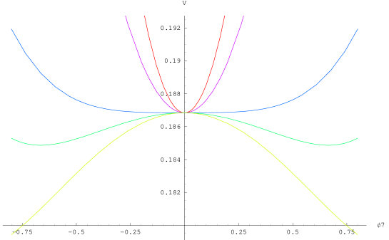
Figure 1: Scalar potential for $\phi_{7}$ at the origin. The ratio $\alpha/\gamma$ is respectively $2$, $1$, $0.9$, $0.8$ and $0.7$ from the red to the yellow curve.

For $\phi_{7}$ larger than (6) the theory has a runaway behaviour, parametrized by $\phi_{7}\rightarrow\infty$,

$$\phi_{1}\sim\sqrt{\frac{f}{2}}\ \ \ \ \ \phi_{2}\sim\sqrt{\frac{f}{2}}\frac{\alpha^{2}}{2\gamma\mu^{2}}\phi_{7}^{2}\ \ \ \ \ \phi_{4}\sim 0\ \ \ \ \ \phi_{5}\sim\sqrt{\frac{f}{2}}\frac{\mu}{\gamma}\frac{1}{\phi_{7}}\ \ \ \ \ \phi_{6}\sim\sqrt{\frac{f}{2}}\frac{\alpha}{2\mu}\phi_{7}$$

$$\phi_{8}\sim\frac{\alpha^{2}}{2\beta\mu^{2}}\phi_{7}^{3}\ \ \ \ \ X\sim\frac{\alpha^{2}}{2\gamma\mu}\phi_{7}^{2}\ \ \ \ \ Z\sim\sqrt{\frac{f}{2}}\frac{\mu^{2}}{\gamma}\frac{1}{\phi_{4}\phi_{7}}$$ (7)

3.2 Two loop corrections

The potential for the field $Z$ is not lifted at one loop, and a two loop analysis is necessary. Considering $Z$ as a background field, the masses of $\phi_{4}$ and $\phi_{5}$ mix. We diagonalize the fermionic mass matrix for these two fields. The rotation is

$$\phi_{4}=-s\theta\rho_{4}+c\theta\rho_{5}$$

$$\phi_{5}=~{}~{}c\theta\rho_{4}+s\theta\rho_{5}$$ (8)

where

$$s\theta^{2}=\frac{h^{2}\mu^{2}-\lambda^{2}_{-}}{\lambda^{2}_{+}-\lambda^{2}_{-}}$$ (9)

and

$$\lambda^{2}_{\mp}=\frac{h^{2}}{2}\left(Z^{2}+2\mu^{2}\mp Z\sqrt{Z^{2}+4\mu^{2}}\right)$$ (10)

The contributions to the two loop effective potential for $Z$ are computed with the same strategy of [16], which is reviewed in Appendix A. The three contributions are given in Figure 4 and are called $V_{SS}$, $V_{SSS}$ and $V_{FFS}$. We found

$$V_{SS} = h^{2}\beta^{2}c\theta^{2}\left(f_{SS}(h^{2}(\mu^{2}-f),\lambda^{2}_{-})+f_{SS}(h^{2}(\mu^{2}+f),\lambda^{2}_{-})-2f_{SS}(h^{2}\mu^{2},\lambda^{2}_{-})\right)$$

$$+\left(c\theta^{2},\lambda_{-}\leftrightarrow s\theta^{2},\lambda_{+}\right)$$

$$V_{SSS} = h^{4}\mu^{2}(s\theta^{2}\beta^{2}+c\theta^{2}\gamma^{2})(f_{SSS}(0,h^{2}(\mu^{2}-f),\lambda^{2}_{-})+f_{SSS}(0,h^{2}(\mu^{2}+f),\lambda^{2}_{-})$$

$$-2f_{FSS}(0,h^{2}\mu^{2},\lambda^{2}_{-}))+\left(s\theta^{2},c\theta^{2},\lambda_{-}\leftrightarrow c\theta^{2},s\theta^{2},\lambda_{+}\right)$$

$$V_{FFS} = h^{2}(\beta^{2}c\theta^{2})(f_{FSS}(0,\lambda^{2}_{-},h^{2}(\mu^{2}-f))+f_{FSS}(0,\lambda^{2}_{-},h^{2}(\mu^{2}+f))$$ (11)

$$-2f_{FSS}(0,\lambda^{2}_{-},h^{2}\mu^{2}))+\left(c\theta^{2},\lambda_{-}\leftrightarrow s\theta^{2},\lambda_{+}\right)$$

Expanding the two loop effective potential for small $Z$, the mass term at the origin is

$$m_{Z}^{2}=h^{6}\mu^{2}(\beta^{2}f(\tau^{2})-\gamma^{2}g(\tau^{2}))$$ (12)

where

$$\tau^{2} =f/\mu^{2}$$ (13)

$$f(x) =-2-\frac{(1-x)^{2}}{x}\log(1-x)+\frac{(1+x)^{2}}{x}\log(1+x)$$

$$g(x) =2+\frac{(1-x)}{x}\log(1-x)-\frac{(1+x)}{x}\log(1+x)$$ (14)

and the functions $f(x)$ and $g(x)$ are positive for $x<1$. There is a regime of the parameters for which this mass term is negative. This happens in the region where

$$\frac{\beta}{\gamma}<\sqrt{\frac{g(\tau^{2})}{f(\tau^{2})}}$$

as in Figure 2. In such a regime of the parameter we look for a minimum of the two loop scalar potential. We indeed observe in Figure 3, by plotting the scalar potential, that there is a choice of the ratio $\beta/\gamma$ where the scalar potential has a minimum at $\langle Z\rangle\neq 0$.

Figure 2: Function $\sqrt{\frac{g(\tau^{2})}{f(\tau^{2})}}$. The region of interest is the one below the curve.

We can then conclude that the model (4) spontaneously breaks $R$-symmetry at two loop in a non supersymmetric (metastable) vacuum. All the tree level flat directions of the scalar potential are lifted by quantum effects. The vacuum is metastable because the field $\phi_{7}$, which acquires positive squared mass around the origin through one loop corrections, develops a runaway in the large vev region. The effective potential for $\phi_{7}$ has to be analyzed to estimate the lifetime of the vacuum.

4 Conclusions

In this note we found a supersymmetry breaking model in which $R$-symmetry is spontaneously broken at two loop in the scalar potential. It is a model of pure chiral fields without any gauge symmetry. There is a tuning in the superpotential, since we did not consider all the terms invariant under the global symmetries of the theory. Adding the allowed term should spoil some of the infrared properties, i.e. supersymmetry breaking.

The tuning problem can be solved by embedding the superpotential in a quiver gauge theory, see Appendix B. In this case the pure chiral fields model has to be considered as the effective theory around the non supersymmetric vacuum found at tree level in the gauge theory, as in [1]. This embedding might also stabilize the runaway behavior in the large field region, where strong dynamics effects of the gauge groups add non perturbative terms to the superpotential.

Moreover, this two loop analysis can be applied to many models with metastable vacua. In most of them an approximate $R$-symmetry exists at such vacua. Two loop effects can offer a solution for this problem. Indeed, as in the model we studied, we can couple the theory to an $R$-charged pseudomodulus that receives two loop corrections from the supersymmetry breaking sector. This field can acquire a quantum scalar potential that breaks spontaneously $R$-symmetry.

Another possibility is to build a model with a “tension” between the one loop and the two loop contributions for some pseudomoduli. This competition could shift the minimum from the origin, breaking $R$-symmetry. In [16] the one and two loop corrections in the ISS model with a mass hierarchy among the fundamental fields have been studied. However in that case one can check that the quantum corrections lead to a runaway, without any local minimum, and then restore supersymmetry. It would be interesting to find models where the combination of one loop and two loop quantum corrections lead to metastable vacua.

Figure 3: Scalar potential for $Z$, plotted for different values of the ratio $\beta/\gamma$, respectively $0.7$, $0.65$, $0.6$ and $0.55$, from left to right. The ration $f/\mu^{2}$ has been chosen to be $0.5$

Appendix A Two loop effective potential

The calculation of the two loop effective potential for a pseudomodulus is involved, since a lot of graphs can contribute. Here we used the trick of [16], which makes the calculation simpler. One has to switch off the supersymmetry breaking scale, $f$, and compute the supersymmetric masses for all the fields. The pseudomoduli are massless also in this supersymmetric version of the model, but in this case they cannot be lifted by quantum corrections. The two loop potential for these fields can be calculated by subtracting the supersymmetric part to the non supersymmetric one. In formulas, calling $V^{(2)}(Z)$ the two loop potential, it is given by

$$V^{(2)}(Z)=V_{nonSUSY}^{(2)}(Z)-V_{SUSY}^{(2)}(Z)$$ (15)

This formula means that the effective potential for $Z$ is due to the diagrams that depends both on the fields whose masses split in the non supersymmetric case (to respect to the supersymmetric one) and on the fields whose masses depend on Z.

There are only few diagrams of this form and they are computed using the formulas of [18, 19].

Figure 4: Relevant Feynman graphs to the two loop potential

In this paper, the model (4) gives rise to three different diagrams, $V_{SS}$, $V_{SSS}$ and $V_{FFS}$, and they are given in Figure 4.

A.1 Details on the calculation

Here we explain the details on the computation of the mass for the pseudomodulus $Z$ around the origin. The potential is made of three different pieces

$$V^{(2)}(Z)=V_{SS}+V_{SSS}+V_{FFS}$$ (16)

They come from three different Feynman graphs, and they have been explicitly derived in [18, 19]. They are

$$V_{SS}(x,y)=J(x)J(y)$$

$$V_{SSS}(x,y,x)=-I(x,y,z)$$

$$V_{FFS}(x,y,z)=J(x)J(y)-J(x)J(z)-J(y)J(z)+(x+y-z)I(x,y,z)$$ (17)

where

$$J(x)=x\left(\log\frac{x}{Q^{2}}-1\right)$$ (18)

In our calculation one argument of the function $I(x,y,z)$ is always zero. We give the expression for this simplified case

$$I(0,x,y)= (x-y)\left(\text{Li}_{2}(y/x)-\log(x/y)\log\frac{x-y}{Q^{2}}+\frac{1}{2}\log^{2}\frac{x}{Q^{2}}-\frac{\pi^{2}}{6}\right)$$

$$- \frac{5}{2}(x+y)+2x\log\frac{x}{Q^{2}}+2y\log\frac{y}{Q^{2}}-x\log\frac{x}{Q^{2}}\log\frac{y}{Q^{2}}$$ (19)

Using these formulas we found in (12) that the mass term for $Z$ is $m_{Z}^{2}=m_{Z_{\beta}}^{2}+m_{Z_{\gamma}}^{2}$, with $\tau^{2}=\frac{f}{\mu^{2}}$,

$$m_{Z_{\beta}}^{2} =\frac{h^{6}\beta^{2}\mu^{2}}{\tau^{2}}\left(\phantom{\frac{\frac{a}{b}}{\frac{c}{c}}}\!\!\!\!\!\!-2\tau^{2}-(1-\tau^{2})^{2}\log(1-\tau^{2})+(1+\tau^{2})^{2}\log(1+\tau^{2})\right.$$

$$+ \left.\frac{1}{2}\log^{2}{(1+\tau^{2})}+Li_{2}(-\tau^{2})+Li_{2}\left(\frac{\tau^{2}}{1+\tau^{2}}\right)\right)$$ (20)

and

$$m_{Z_{\gamma}}^{2}=-\frac{h^{6}\gamma^{2}\mu^{2}}{\tau^{2}}(2\tau^{2}+(1-\tau^{2})\log(1-\tau^{2})-(1+\tau^{2})\log(1+\tau^{2})))$$ (21)

The last line in (A.1) vanishes for $\tau^{2}<1$ because of an identity of dilogarithms.

Appendix B Embedding in quiver gauge theories

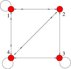
Figure 5: Quiver for the superpotential (B.1).

A possible embedding in quiver gauge theory is a four $U(1)$ nodes theory (note that also non-abelian groups are admitted) with superpotential

$$W =q_{12}^{(1)}q_{21}^{(1)}X_{11}-fX_{11}+\mu\left(q_{12}^{(1)}q_{21}^{(2)}+q_{12}^{(2)}q_{21}^{(1)}\right)+q_{21}^{(1)}q_{14}^{(7)}q_{42}^{(6)}$$

$$+ q_{12}^{(1)}q_{24}^{(6)}q_{41}^{(7)}+q_{21}^{(2)}q_{14}^{(7)}q_{42}^{(5)}+q_{12}^{(2)}q_{24}^{(5)}q_{41}^{(7)}+q_{21}^{(1)}q_{14}^{(8)}q_{42}^{(5)}$$

$$+ q_{12}^{(1)}q_{24}^{(5)}q_{41}^{(8)}+q_{23}^{(4)}Z_{33}q_{32}^{(4)}+q_{43}q_{32}^{(4)}q_{24}^{(5)}+q_{42}^{(5)}q_{23}^{(4)}q_{34}+q_{34}Y_{44}q_{43}-\mu^{2}Y_{44}$$ (22)

The quiver is shown in Figure 5. The upper scripts map the fields in (22) with the corresponding fields in (4). The fields $q_{34}$ and $q_{43}$ get a vev $\mu$ from the equation of motion of the field $Y_{44}$. This gives a mass term for the fields $q_{32}^{(4)}q_{24}^{(5)}$ and $q_{42}^{(5)}q_{23}^{(4)}$, as in (4).

In this model the requirement of gauge invariance forbids the dangerous term $X\phi_{5}\phi_{6}$ that we discussed in section 3.

References

- [1] K. A. Intriligator, N. Seiberg and D. Shih, JHEP 0604 (2006) 021 [arXiv:hep-th/0602239].
- [2] S. Franco and A. M. Uranga, JHEP 0606 (2006) 031 [arXiv:hep-th/0604136]. H. Ooguri and Y. Ookouchi, Nucl. Phys. B 755 (2006) 239 [arXiv:hep-th/0606061]. S. Forste, Phys. Lett. B 642 (2006) 142 [arXiv:hep-th/0608036]. M. Dine, J. L. Feng and E. Silverstein, Phys. Rev. D 74 (2006) 095012 [arXiv:hep-th/0608159]. R. Argurio, M. Bertolini, S. Franco and S. Kachru, JHEP 0701 (2007) 083 [arXiv:hep-th/0610212]. and JHEP 0706 (2007) 017 [arXiv:hep-th/0703236]. I. Garcia-Etxebarria, F. Saad and A. M. Uranga, JHEP 0705 (2007) 047 [arXiv:0704.0166 [hep-th]]. S. Hirano, JHEP 0705 (2007) 064 [arXiv:hep-th/0703272]. R. Essig, K. Sinha and G. Torroba, JHEP 0709 (2007) 032 [arXiv:0707.0007 [hep-th]]. A. Giveon and D. Kutasov, Nucl. Phys. B 796 (2008) 25 [arXiv:0710.0894 [hep-th]]. M. Buican, D. Malyshev and H. Verlinde, JHEP 0806 (2008) 108 [arXiv:0710.5519 [hep-th]]. A. Amariti, D. Forcella, L. Girardello and A. Mariotti, arXiv:0803.0514 [hep-th].
- [3] A. Amariti, L. Girardello and A. Mariotti, JHEP 0612 (2006) 058 [arXiv:hep-th/0608063]
- [4] M. Dine and J. Mason, Phys. Rev. D 77, 016005 (2008) [arXiv:hep-ph/0611312]. C. Csaki, Y. Shirman and J. Terning, JHEP 0705, 099 (2007) [arXiv:hep-ph/0612241]. H. Murayama and Y. Nomura, Phys. Rev. Lett. 98 (2007) 151803 [arXiv:hep-ph/0612186]. O. Aharony and N. Seiberg, JHEP 0702 (2007) 054 [arXiv:hep-ph/0612308]. A. Amariti, L. Girardello and A. Mariotti, Fortsch. Phys. 55, 627 (2007) [arXiv:hep-th/0701121]. T. Kawano, H. Ooguri and Y. Ookouchi, Phys. Lett. B 652 (2007) 40 [arXiv:0704.1085 [hep-th]]. J. E. Kim, Phys. Lett. B 651 (2007) 407 [arXiv:0706.0293 [hep-ph]]. A. Amariti, L. Girardello and A. Mariotti, JHEP 0710 (2007) 017 [arXiv:0706.3151 [hep-th]]. J. E. Kim, Phys. Lett. B 651 (2007) 407 [arXiv:0706.0293 [hep-ph]]. N. Haba and N. Maru, Phys. Rev. D 76 (2007) 115019 [arXiv:0709.2945 [hep-ph]]. M. Dine and J. D. Mason, arXiv:0712.1355 [hep-ph]. S. A. Abel, C. Durnford, J. Jaeckel and V. V. Khoze, JHEP 0802 (2008) 074 [arXiv:0712.1812 [hep-ph]]. R. Kitano and Y. Ookouchi, arXiv:0812.0543 [hep-ph]. S. Abel, J. Jaeckel, V. V. Khoze and L. Matos, arXiv:0812.3119 [hep-ph]. R. Essig, J. F. Fortin, K. Sinha, G. Torroba and M. J. Strassler, arXiv:0812.3213 [hep-th].
- [5] R. Kitano, H. Ooguri and Y. Ookouchi, Phys. Rev. D 75 (2007) 045022 [arXiv:hep-ph/0612139].
- [6] D. Shih, JHEP 0802 (2008) 091 [arXiv:hep-th/0703196].
- [7] Z. Sun, arXiv:0810.0477 [hep-th].
- [8] K. A. Intriligator, N. Seiberg and D. Shih, JHEP 0707 (2007) 017 [arXiv:hep-th/0703281]. L. Ferretti, JHEP 0712 (2007) 064 [arXiv:0705.1959 [hep-th]]. H. Y. Cho and J. C. Park, JHEP 0709 (2007) 122 [arXiv:0707.0716 [hep-ph]]. S. Abel, C. Durnford, J. Jaeckel and V. V. Khoze, Phys. Lett. B 661 (2008) 201 [arXiv:0707.2958 [hep-ph]]. H. Abe, T. Kobayashi and Y. Omura, JHEP 0711 (2007) 044 [arXiv:0708.3148 [hep-th]]. L. G. Aldrovandi and D. Marques, JHEP 0805 (2008) 022 [arXiv:0803.4163 [hep-th]]. K. R. Dienes and B. Thomas, arXiv:0806.3364 [hep-th].
- [9] L. Girardello and M. T. Grisaru, Nucl. Phys. B 194 (1982) 65.
- [10] S. Ferrara, L. Girardello and F. Palumbo, Phys. Rev. D 20 (1979) 403.
- [11] S. D. L. Amigo, A. E. Blechman, P. J. Fox and E. Poppitz, arXiv:0809.1112 [hep-ph].
- [12] A. E. Nelson and N. Seiberg, Nucl. Phys. B 416, 46 (1994) [arXiv:hep-ph/9309299].
- [13] D. Marques and F. A. Schaposnik, JHEP 0811 (2008) 077 [arXiv:0809.4618 [hep-th]].
- [14] J. Bagger, E. Poppitz and L. Randall, Nucl. Phys. B 426, 3 (1994) [arXiv:hep-ph/9405345].
- [15] A. Giveon, A. Katz, Z. Komargodski and D. Shih, JHEP 0810 (2008) 092 [arXiv:0808.2901 [hep-th]].
- [16] A. Giveon, A. Katz and Z. Komargodski, JHEP 0806 (2008) 003 [arXiv:0804.1805 [hep-th]].
- [17] K. Intriligator, D. Shih and M. Sudano, arXiv:0809.3981 [hep-th].
- [18] C. Ford, I. Jack and D. R. T. Jones, Nucl. Phys. B 387 (1992) 373 [Erratum-ibid. B 504 (1997) 551] [arXiv:hep-ph/0111190].
- [19] S. P. Martin, Phys. Rev. D 65 (2002) 116003 [arXiv:hep-ph/0111209].