A randomized polynomial-time algorithm
for the Spanning Hypertree Problem on 3-uniform hypergraphs

Abstract

Consider the problem of determining whether there exists a spanning hypertree in a given $k$-uniform hypergraph. This problem is trivially in $\mathsf{P}$ for $k=2$, and is $\mathsf{NP}$-complete for $k\geq 4$, whereas for $k=3$, there exists a polynomial-time algorithm based on Lovász’ theory of polymatroid matching.

Here we give a completely different, randomized polynomial-time algorithm in the case $k=3$. The main ingredients are a Pfaffian formula by Vaintrob and one of the authors (G.M.) for a polynomial that enumerates spanning hypertrees with some signs, and a lemma on the number of roots of polynomials over a finite field.

I Introduction

A (finite) hypergraph $G=(V,E)$ consists of a finite set $V$ (the vertex set) and a set $E$ of subsets of $V$ (the hyperedges), each of cardinality at least 2. We also write $V(G)=V$ and $E(G)=E$. When all the hyperedges have the same cardinality $k$, we say that the hypergraph is $k$-uniform. In the case $k=2$ we are dealing with ordinary (simple) graphs. We say that $H\subseteq G$ is a sub-hypergraph if $V(H)\subseteq V(G)$ and $E(H)\subseteq E(G)$; a sub-hypergraph is spanning if $V(H)=V(G)$. A hypergraph $H$ is a hypertree if it is connected and there are no cyclic sequences of vertices and hyperedges

$$v_{1},A_{1},v_{2},A_{2},\cdots,v_{\ell},A_{\ell},v_{\ell+1}\quad(v_{\ell+1}=v_{1})$$

such that $\ell\geq 2$, $v_{i}\neq v_{i+1}$ and $v_{i},v_{i+1}\in A_{i}$. An example of a 3-uniform hypergraph, together with a spanning sub-hypergraph that is a hypertree, is shown in Figure 1.

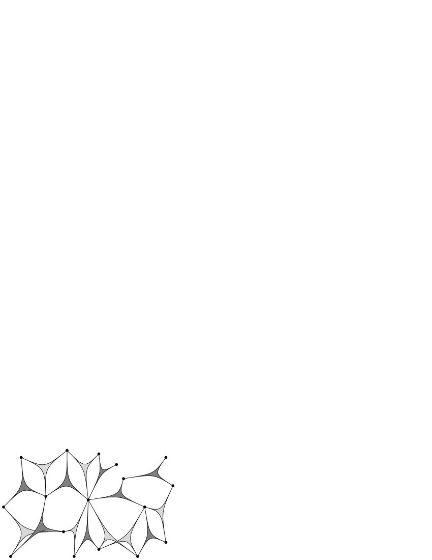
Figure 1: A 3-uniform hypergraph $G$, and a spanning hypertree $T\subset G$, whose edges are in darker gray.

We will deal here with issues in Computational Complexity Theory GJ . An introduction to the subject which includes the class $\mathsf{RP}$ of probabilistic polynomial-time problems, pertinent to this paper, can be found in Chapters 2–4 of Talbot and Welsh talbotwelsh .

In this paper we are concerned with the following decision problem:

$k$-Uniform Spanning Hypertree ($k$-SHT):

Given a $k$-uniform hypergraph $G=(V,E)$, determine whether there exists a spanning hypertree.

Of course, every connected graph contains a spanning tree, so $k$-SHT is trivially in $\mathsf{P}$ for $k=2$ (it suffices to check whether $G$ is connected). On the other hand, for $k\geq 3$ it is not true that every connected $k$-uniform hypergraph contains a spanning hypertree, and the decision problem is highly nontrivial.

Our main result here is to provide an $\mathsf{RP}$ algorithm for the $k$-Uniform Spanning Hypertree problem when $k=3$. After a first version of this paper was completed, we have learnt from Andras Sebö that there is actually a polynomial-time algorithm for this problem, coming as a specialization of Lovász’ algorithm for matching on linear 2-polymatroids Lov1 ; Lov2 . However, Lovász’ techniques are completely different from ours, and we believe that our more algebraic approach is of independent interest. We remark that for $k\geq 4$ the spanning hypertree problem is $\mathsf{NP}$-complete by a result of C. Thomassen which appears in (af, , Theorem 4). (We thank Marc Noy for bringing this argument to our attention.) Moreover, the same argument shows that the corresponding counting problem is $\sharp$$\mathsf{P}$-complete already for $k\geq 3$. We will briefly review Thomassen’s argument at the end of this introduction.

Organization of the paper. The bulk of this paper has two parts. In the first part, we discuss the main ingredient of our $\mathsf{RP}$ algorithm, namely the Pfaffian-Tree Theorem of masvain2 which expresses a signed version of the multivariate spanning-tree generating function of a $3$-uniform hypergraph as a Pfaffian. Then in the second part, we describe our algorithm, first intuitively, and then more formally, and sketch the analysis of time- and space-complexity. This part is fairly standard in complexity theory, but we hope that the partly expository presentation of the various concepts involved will be useful for the interdisciplinary audience (such as ourselves) we have in mind. Finally, we end the paper with some speculations and directions for further research suggested by our work.

To conclude this introduction, here is, then, Thomassen’s argument showing that k-SHT is $\mathsf{NP}$-complete for $k\geq 4$.

We recall that an exact cover in a hypergraph $G=(V,E)$ is a subset $E^{\prime}\subseteq E$ of the hyperedges such that every vertex of $G$ belongs to exactly one hyperedge in $E^{\prime}$. (In the special case where $G$ is an ordinary graph, an exact cover is nothing but a perfect matching.) Now consider the following decision problem:

Exact cover by $k$-sets (X$k$C):

Given a $k$-uniform hypergraph $G=(V,E)$, determine whether there exists an exact cover.

X3C is known to be $\mathsf{NP}$-complete, and is classified as problem [​[SP2]​] in Garey and Johnson GJ . (It is $\mathsf{NP}$-complete even when restricted to 3-partite hypergraphs, in this case being called 3-Dimensional Matching (3DM, [​[SP1]​]).) Implicitly, analogous statements hold as well for any $k\geq 3$. Conversely, X2C is polynomial, by matching techniques, even in its optimization variant, e.g. by Gallai-Edmonds algorithm (see LovPlu ). On the other hand, the corresponding counting problem (equivalently: counting perfect matchings on arbitrary graphs), is known to be $\sharp$$\mathsf{P}$-complete (Valiant V ).

Now, given an arbitrary $k$-uniform hypergraph $G$, Thomassen constructs a $(k+1)$-uniform hypergraph $G^{\prime}$ as follows: add an extra vertex $\star$, and let

$$E(G^{\prime})=\{e\cup\{\star\}\,|\,e\in E(G)\}\,.$$

The key observation is that spanning hypertrees of $G^{\prime}$ correspond bijectively to exact covers of $G$ (with the obvious bijection, namely deleting $\star$ from each hyperedge). Thus, any algorithm for $(k+1)$-SHT provides an algorithm for X$k$C. In other words, X$k$C is reducible to $(k+1)$-SHT.

From what we said above about X$k$C, it follows that $k$-SHT is $\mathsf{NP}$-complete for $k\geq 4$, and counting spanning hypertrees in a 3-uniform hypergraph is $\sharp$$\mathsf{P}$-complete, as asserted.

II A Pfaffian formula

Let $G=(V,E)$ be a finite hypergraph on $N$ vertices. The multivariate generating function for spanning hypertrees on $G$ is

$$Z_{G}(\vec{w})=\sum_{T\in\mathcal{T}(G)}\prod_{A\in E(T)}w_{A}\,,$$ (1)

where $\mathcal{T}(G)$ is the set of spanning hypertrees of $G$, and the $w_{A}$ are commuting indeterminates, one for each hyperedge $A\in E(G)$.

Assume that $G$ is $k$-uniform. If $G$ has a spanning hypertree, then necessarily

$$N=(k-1)n+1\leavevmode\nobreak\ ,$$ (2)

where $n$ is the number of hyperedges in each spanning hypertree. Therefore we will assume (2) from now on.

It will be convenient to consider $G$ as a sub-hypergraph of $\mathcal{K}(N,k)$, the complete $k$-uniform hypergraph on $N$ vertices, which has an hyperedge for all unordered $k$-uples $A=\{i_{1},\ldots,i_{k}\}\subseteq[N]:=\{1,2,\ldots,N\}$. We denote $Z_{\mathcal{K}(N,k)}(\vec{w})$ by $Z_{n,k}(\vec{w})$, and $\mathcal{T}(\mathcal{K}(N,k))$ by $\mathcal{T}_{n,k}$. Note that the degree of $Z_{n,k}(\vec{w})$ is $n$, as given in (2). The spanning hypertree generating function $Z_{G}(\vec{w})$ of an arbitrary $k$-uniform hypergraph $G$ can be obtained from $Z_{n,k}(\vec{w})$ by setting the weights $w_{A}$ to zero for hyperedges $A$ not in $G$.

A classical result by Kirchhoff is that, for $k=2$, the expression $Z_{n,2}(\vec{w})$ (and therefore $Z_{G}(\vec{w})$ for any graph $G$) is given by a determinant. Defining the $N\times N$ Laplacian matrix $L$ as

$$L_{ij}=\left\{\begin{array}[]{ll}-w_{ij}&i\neq j\\ \sum_{k\neq i}w_{ik}&i=j\end{array}\right.$$ (3)

and taking a whatever $(N-1)$-dimensional principal minor $L(i_{0})$ (i.e. with row and column $i_{0}$ removed – and remark that $N-1=n$ if $k=2$), one has

Theorem 1 (Matrix-Tree)

$$Z_{n,2}(\vec{w})=\det L(i_{0})\,.$$ (4)

As is well-known, Kirchhoff’s formula allows one to count spanning trees on a graph $G$: putting $w_{A}=1$ if $A\in E(G)$ and $w_{A}=0$ otherwise, the determinant (4) gives the cardinality of the set $\mathcal{T}(G)$ of spanning trees on $G$. For later use, we remark that this formula also shows that counting spanning trees on graphs is in $\mathsf{P}$, as determinants can be evaluated in polynomial time.

For general $k$-uniform hypergraphs, no such formula is known if $k\geq 3$. Moreover, a determinantal expression for $Z_{n,k}(\vec{w})$ is unlikely to exist, since counting spanning hypertrees is $\sharp$$\mathsf{P}$-complete if $k\geq 3$, as discussed in the introduction.

We remark in passing that, nevertheless, the number of spanning hypertrees on the complete hypergraph $\mathcal{K}(N,k)$ is known: generalizing the classical result by Cayley for $k=2$, one has that

$$|\mathcal{T}_{n,k}|=\frac{\big{(}(k-1)n\big{)}!}{\big{(}(k-1)n+1\big{)}\,n!}\left(\frac{(k-1)n+1}{(k-1)!}\right)^{n}\,,$$ (5)

as can be found in noibedini (see also references therein).

From now on, we will consider the case $k=3$. Our starting point is a recent result, due to A. Vaintrob and one of the authors (G.M.) masvain2 , which states that an alternating sign version of the spanning hypertree generating function $Z_{n,3}(\vec{w})$ is given by a Pfaffian.

We will denote this modified polynomial by $Z^{\star}_{n,3}(\vec{w})$. For a given ordering of the vertices of the hypergraph (or, equivalently, a labeling of the vertices with integers from $1$ to $N$), a sign function $\epsilon(T)$ for hypertrees $T$ is defined (more details are given later); then

$$Z^{*}_{n,3}(\vec{w})=\sum_{T\in\mathcal{T}_{n,3}}\epsilon(T)\prod_{A\in E(T)}w_{A}\,.$$ (6)

To state the result, let $\epsilon_{ijk}$ be the totally antisymmetric tensor (i.e. $\epsilon_{ijk}=0$ if two or more indices are equal, $\epsilon_{ijk}=1$ if $i<j<k$ or any other cyclic permutation, and $\epsilon_{ijk}=-1$ if $i<k<j$ or any other cyclic permutation) and define a $N$-dimensional antisymmetric matrix $\Lambda$, with off-diagonal elements

$$\Lambda_{ij}=\sum_{k\neq i,j}\epsilon_{ijk}w_{\{i,j,k\}}\leavevmode\nobreak\ .$$ (7)

Then one has, for any principal minor $\Lambda(i_{0})$:

Theorem 2 (Pfaffian-Hypertree masvain2 )

$$Z^{*}_{n,3}(\vec{w})=(-1)^{i_{0}-1}\,\mathrm{Pf}\,\Lambda(i_{0})\,.$$ (8)

(The original formulation in masvain2 uses indeterminates $y_{ijk}$ which are antisymmetric in their indices. The correspondence with our notation here is simply that $y_{ijk}=\epsilon_{ijk}w_{\{i,j,k\}}$.)

In order to give meaning to equations (6) and (8), we must define the sign function $\epsilon(T):\mathcal{T}_{n,3}\to\{\pm 1\}$. Several equivalent definitions exist, and all of them require making some arbitrary choices; the proof that the resulting sign is actually independent of these choices (developed to full extent in masvain2 ) can be performed inductively in tree size, studying the invariances in the elementary step of adding a ‘leaf’ edge to a tree.

It is worth stressing, however, that the precise determination of this sign function is not actually used in our algorithm (and not even in our proofs of complexity bounds).

The first definition of $\epsilon(T)$ given in masvain2 is as follows. For $S\subseteq[N]$, call $\tau_{S}$ the permutation which rotates cyclically the elements of $S$ (in their natural order), and keeps fixed the others. Then, for a given ordered $n$-uple of hyperedges $(A_{1},\ldots,A_{n})$ forming a tree $T$, define the permutation $\hat{\tau}=\tau_{A_{1}}\cdots\tau_{A_{n}}$. This permutation is composed of a single cycle of length $N$. It is thus conjugated to the “canonical” $N$-cycle $\tau_{[N]}$, i.e. there exists $\sigma$ such that

$$\hat{\tau}=\sigma\,\tau_{[N]}\,\sigma^{-1}\,.$$ (9)

Then actually the signature $\epsilon(\sigma)$ does not depend on the ordering of the hyperedges, but only on $T$, and taking $\epsilon(T):=\epsilon(\sigma)$ is a valid definition, and the appropriate one for (8) to hold.

An equivalent definition is as follows. Consider a planar embedding of the tree, in such a way that for each hyperedge $A_{\alpha}$, if $(i_{\alpha},j_{\alpha},k_{\alpha})$ denote its three vertices cyclically ordered in the clockwise order given by the embedding, one has $\epsilon_{ijk}=1$. (Such an embedding always exists.) Then construct the string $\hat{\rho}$ of $3n$ symbols in $[N]$ (recall that $n$ is the number of hyperedges) corresponding to the sequence of vertices visited by a clockwise path surrounding the tree, starting from an arbitrary vertex. Each of the $N$ vertices occurs in this string, but some vertices appear more than once. Now remove entries from this string until each of the $N$ vertices appears exactly once, thus getting a string $\rho$ of $N$ distinct elements of $[N]$. If we interpret this string as a permutation, then $\epsilon(T)=\epsilon(\rho)$, despite of the arbitrariness of the choices for the planar embedding, the starting point and the extra entries we choose to remove. An example is given in (masvain2, , Figure 3.1).

Instead of using a planar embedding, one can also describe this procedure by choosing a given vertex as root (say, $i_{0}$), and orienting the edges accordingly (so that each edge has a “tip” and two “tail” vertices, and all edges are oriented towards the root). Now the vertices inside any hyperedge $A_{\alpha}$ can be uniquely ordered $(i_{\alpha},j_{\alpha},k_{\alpha})$ such that $i_{\alpha}$ is the tip and $\epsilon_{i_{\alpha}j_{\alpha}k_{\alpha}}=1$. With this notation, the sign $\epsilon(T)$ coincides with the sign of a certain monomial in the $N$-dimensional exterior algebra (or real Grassmann Algebra):

$$e(i_{0})\wedge\Big{(}\bigwedge_{\alpha}e(j_{\alpha})\wedge e(k_{\alpha})\Big{)}=\epsilon(T)\;e(1)\wedge\cdots\wedge e(N)\,.$$ (10)

In order to see the equivalence with the previous definition of $\epsilon(T)$, it suffices to take an appropriate planar embedding of $T$ and to observe that we can perform the removal of extra entries in such a way that in the final string $\rho$, the two tails of each hyperedge always come consecutively. The ordering of the hyperedges in the product on the L.H.S. of (10) is irrelevant at sight, as an hyperedge with odd size has an even number of tails, which thus are commuting expressions in exterior algebra. Nonetheless the true invariance is stronger, as it concerns also the choice of the root vertex, and much more, as implied by the preceeding paragraphs. The expression (10) above is an efficient way of computing $\epsilon(T)$ for a given tree $T$.

This last definition for $\epsilon(T)$ has also the advantage of driving us easily towards a proof using Grassmann variables of formula (8). In fact, for both equations (4) and (8), say with $i_{0}=1$, we can recognize the expressions for Gaussian integrals of Grassmann variables, “complex” and “real” in the two cases respectively

$$Z_{n,2}(\vec{w}) =\int\mathcal{D}(\psi,{\bar{\psi}})\;{\bar{\psi}}_{1}\psi_{1}\,e^{\sum w_{ij}({\bar{\psi}}_{i}-{\bar{\psi}}_{j})(\psi_{i}-\psi_{j})}\,;$$ (11)

$$Z^{*}_{n,3}(\vec{w}) =\int\mathcal{D}(\theta)\;\theta_{1}\,e^{\sum w_{ijk}(\theta_{i}\theta_{j}+\theta_{j}\theta_{k}+\theta_{k}\theta_{i})}\,.$$ (12)

It is combinatorially clear that such an integral will generate an expansion in terms of spanning subgraphs, with one component being a rooted tree and all the others being unicyclic. Then one realizes that, because of the anticommutation of the variables, unicyclics get contributions with opposite signs, which ultimately cancel out. However this mechanism occurs in slightly different ways in the two cases (cfr. usPRL and abdes respectively for more details).

Remark. The original proof of the Pfaffian-hypertree theorem in masvain2 was by induction on the number of hyperedges using a contraction-deletion formula. Another proof was given in masvain which exploits the knot-theoretical context which originally lead to the discovery of the formula. The proof using Grassmann variables alluded to above is due to Abdesselam abdes . Finally, yet another proof was given by Hirschman and Reiner HR using the concept of a sign-reversing involution.

III Towards a Randomized Polynomial-time algorithm

Equation (6) provides us with a multivariate alternating-sign generating function, which is a polynomial, and identically vanishing if and only if our hypergraph $G$ has no spanning hypertrees. Can we use this to decide efficiently whether $G$ has a spanning hypertree?

Recall that in the classical Matrix-Tree theorem for ordinary graphs there are no signs, and upon putting edge weights equal to $1$ for edges in the graph, and equal to zero otherwise, we get the number of spanning trees on our graph. Moreover, calculating numerically the determinant of a matrix can be performed by Gaussian elimination in polynomial time.

Let us apply the same idea to the Pfaffian-Hypertree formula (8). Since $\det\Lambda(i_{0})=(\mathrm{Pf}\,\Lambda(i_{0}))^{2}$, we can again evaluate $Z^{*}_{n,3}(\vec{w})$ in polynomial time, if, as before, we set the hyperedge weights equal to $1$ for hyperedges in a $3$-uniform hypergraph $G$, and equal to zero otherwise. But because of the signs in $Z^{*}_{n,3}$, this is not the number of spanning hypertrees in $G$!

One way out is to evaluate $\det\Lambda(i_{0})$ at some random set of numerical weights (but keeping weights equal to zero for hyperedges not in the hypergraph). If one gets a non-zero result, this would certainly prove that the multivariate generating function is non-zero, and hence provide a certificate of the fact that a spanning hypertree exists. Conversely, if many evaluations at random independent points are zero, one starts believing that the graph has no hypertrees at all. This naïve idea can be formalized within the framework of the $\mathsf{RP}$ complexity class.

In complexity theory, the class of Randomized Polynomial-time problems ($\mathsf{RP}$) contains problems for which, given any instance, a polynomial-time probabilistic algorithm can be called an arbitrary number of times in such a way that:

• If the correct answer is ‘False’, it always returns ‘False’;

• If the correct answer is ‘True’, then it returns ‘False’ for the $t$-th query with a probability at most $1/2$, regardless of the previous query results.

We now discuss in more detail how to construct an $\mathsf{RP}$-algorithm from the Pfaffian-Hypertree formula (8). Note that, of course, one has $\mathsf{P}$ $\subseteq$ $\mathsf{RP}$ $\subseteq$ $\mathsf{NP}$.

IV Gaussian algorithm over finite fields

Calculating numerically the determinant of a matrix using Gauss elimination is commonly thought to be of polynomial time complexity (at most cubic). If this is certainly true for “float” numbers (but suffers from numerical approximations), some remark is in order for “exact” calculations. Indeed, in this case we have to choose a field, such as $\mathbb{Q}$, which is suitable for exact numerical computation through a sequence of sums, products and inverses, which, in the complexity estimate above, have been considered an “unity of complexity” (a variant is possible, in which one works in the ring $\mathbb{Z}$ and recursively factors out a number of g.c.d.’s). This is however not an innocent assumption. For example, if one works with rational numbers with both numerators and denominators having a bounded number of digits $d$, in general, during the Gauss procedure, one may suffer from an exponential growth of this number (as the l.c.m. of two $d$-digit integers may well have $2d$ digits).

An improved choice, and which makes the analysis simpler, is to consider finite fields $\mathrm{GF}_{q}$, for which the complexity of operations is uniformly bounded. A primer in finite fields can be found, for example, in the textbook bookGF . The field $\mathrm{GF}_{q}$ exists for $q$ a power of a prime, $p^{h}$, as a quotient of a set of polynomials with coefficients in $\mathbb{Z}_{p}$ by a polynomial of degree $h$, irreducible in $\mathbb{Z}_{p}$. Also for finite fields, polynomials of degree $n$ have at most $n$ distinct roots. Recall that $a^{2}=0$ iff $a=0$ in any field, so that also in $\mathrm{GF}_{q}$ one has $\det\Lambda=0$ only if $\mathrm{Pf}\,\Lambda=0$.

Two specially used cases are $q$ prime, in which $\mathrm{GF}_{q}$ just coincides with $\mathbb{Z}_{q}$, equipped with the product modulo $q$, and $q$ a power of 2, which is mostly used in Coding Theory. In both cases, the arithmetic operations $+(\cdot,\cdot)$, $\times(\cdot,\cdot)$ and $1/(\cdot)$ are performed in a very efficient way, if a ‘Space’ requirement of order $q$ is allowed for storing a table of discrete logarithms (this will turn out to be subleading for our problem). As a result, if a given value for $q$ is chosen, calculating the determinant of a $N$-dimensional matrix in $\mathrm{GF}(q)$ takes a time of order $N^{3}(\log q)^{2}$ (improved to $N^{3}\log q$ if a fast preprocessing, concerning the table of logarithms, is performed bookGF ; bookShoup ). Remark that for us it is important to control the dependence not just on $N$ but also on $q$, because in our context $q$ will depend on $N$.

V Roots of polynomials over a finite field

The analysis of the previous sections naturally induces us to study the roots of polynomials over Galois fields $\mathrm{GF}_{q}$. In particular we need an upper bound as follows:

Lemma 1

Let $f(x_{1},\ldots,x_{n})$ be a non-zero polynomial in $n$ variables of total degree $d$ with coefficients in the finite field $\mathrm{GF}_{q}$. Then $f$ has at most $dq^{n-1}$ roots. In other words, the probability that a randomly chosen $(a_{1},\ldots,a_{n})\in\mathrm{GF}_{q}^{n}$ is a root of $f$ is $\leq d/q$.

For the convenience of the reader, we include a proof of this lemma. An essentially equivalent proof formulated in the language of probability theory is given in (talbotwelsh, , Thm. 4.2).

Recall that the field $\mathrm{GF}_{q}$ has $q$ elements. We say that $(a_{1},\ldots,a_{n})\in\mathrm{GF}_{q}^{n}$ is a non-root of $f$ if $f(a_{1},\ldots,a_{n})\neq 0$. We must show that $f$ has at least $(q-d)q^{n-1}$ non-roots.

The proof is by induction on $n$, the number of variables. For $n=1$, a non-zero one-variable polynomial of degree $d$ has at most $d$ roots. Now assume $n\geq 2$. Write

$$f(x_{1},\ldots,x_{n})=\sum_{i=0}^{m}x_{1}^{i}\,g_{i}(x_{2},\ldots,x_{n})\,\leavevmode\nobreak\ ,$$

where $g_{m}\neq 0$ and $m\leq d$. Observe that $g_{m}$ has degree at most $d-m$. By the induction hypothesis applied to $g_{m}$, we know that $g_{m}$ has at most $(d-m)q^{n-2}$ roots, and therefore we can find at least $(q-d+m)q^{n-2}$ non-roots of $g_{m}$. For every $(a_{2},\ldots,a_{n})$ which is a non-root of $g_{m}$, consider

$$f(x_{1},a_{2},\ldots,a_{n})\,.$$

This is a non-trivial polynomial in $x_{1}$ of degree exactly $m$, therefore it has at most $m$ roots and at least $q-m$ non-roots. Thus we have found at least $(q-d+m)q^{n-2}(q-m)$ non-roots of $f$ (namely $(q-d+m)q^{n-2}$ possibilities for $(a_{2},\ldots,a_{n})$ times $q-m$ possibilities for $a_{1}$.) It is easy to check that $(q-d+m)q^{n-2}(q-m)\geq(q-d)q^{n-1}$. This completes the proof. $\square$

VI The algorithm

The lemma 1 stated above implies that, for any $3$-uniform hypergraph $G$ with $2n+1$ vertices, if one evaluates $(Z_{n,3}^{*})^{2}$ at some values $\{w_{A}\}_{A\in E(G)}$ random uniformly sampled from $\mathrm{GF}_{q}$ (and, of course, $w_{A}=0$ if $A\not\in E(G)$), one gets always zero if $G$ has no spanning hypertrees, and obtains zero although $G$ has some spanning hypertrees, with probability at most $n/q$. If $q\geq 2n$, we are within the framework of the $\mathsf{RP}$ complexity class.

So our algorithm is just as follows. Given $G$, choose a root vertex and an ordering (once and for ever), and build the corresponding matrix $\Lambda$ of indeterminates as in (7) (as a matrix of lists of edge-labels, with signs). Build the table of $\mathrm{GF}_{q}$–logarithms for an appropriate value of $q$. Then, for a given fault tolerance $\varepsilon=2^{-k}$, repeat $k$ times the following probabilistic algorithm:

• extract the values $w_{A}$ independently identically distributed in $\mathrm{GF}_{q}$;

• evaluate $\Lambda$ in numerical form for these values;

• evaluate the determinant numerically by Gauss elimination (in $\mathrm{GF}_{q}$);

• if the result is non-zero, return “there are trees”, and break the cycle.

Then, if the cycle terminates without breaking, return “there are no trees with probability $1-2^{-k}$ ”.

If we consider a generic value of $q>n$, when the cycle terminates without breaking we know that there are no trees with probability at least $1-(n/q)^{k}$. For a given value of $\varepsilon$, we thus get an upper bound on the time complexity (up to a multiplicative constant)

$$n^{3}\log q\,\left\lceil\frac{-\log\varepsilon}{\log q-\log n}\right\rceil\,.$$

If both $n,\varepsilon^{-1}\to\infty$, optimization in $q$ suggests to take $q\sim n/\varepsilon$ and perform a single query, (instead of taking $q=2n$ and performing $\mathcal{O}(-\log\varepsilon)$ queries). This saves an extra factor $\min(\log n,-\log\varepsilon)$, and gives a complexity of order $n^{3}\max(\log n,-\log\varepsilon)$.

VII Perspectives

Given the datum of a $3$-uniform hypergraph $G=(V,E)$, a positive integer $s$, and a set of integer-valued edge costs $\{c_{A}\}$, consider the cost function for spanning hypertrees $\mathcal{H}(T)=\sum_{A\in E(T)}c_{A}$. Then, one has the decision problem of determining if $G$ has any spanning hypertree $T$ with $\mathcal{H}(T)\leq s$. This problem is essentially equivalent to the corresponding optimization problem, of finding the spanning hypertree of minimum cost, and has a complexity at least as large as the one of $3$-SHT. At the time of this writing, we don’t know whether Lovász’ polymatroid matching techniques can answer this problem, which is not addressed in Lov1 ; Lov2 . Be that as it may, it would also be interesting to understand if an $\mathsf{RP}$ algorithm exists for this problem, through an extension of the technique described in the present paper.

Another issue worth investigating may be how to use the exact expression for the sign $\epsilon(T)$ and maximize the fraction of terms getting the same sign in (6), in order to use the Pfaffian-Hypertree formula in all of its strength. This may lead to a notion of Pfaffian orientation for 3-uniform hypergraphs, analogous to the notion of Pfaffian orientation (or Kasteleyn orientation) for graphs RST . Indeed, our story is somewhat parallel to the story for perfect matchings (and also Lovász algorithm is a generalization of the Edmonds-Gallai algorithm for matchings on graphs). In particular, if we construct a $3$-uniform hypergraph $G^{\prime}$ from a graph $G$ using the procedure described in the introduction, the Pfaffian-Hypertree formula (8) for $G^{\prime}$ becomes the well-known alternating sign multivariate generating function for perfect matchings of $G$ given by a Pfaffian. Now in the graph case, there is the notion of Kasteleyn orientation which serves to get rid of the signs in the Pfaffian and allows therefore to count perfect matchings in this way. A Kasteleyn orientation exists for planar graphs, but not in general. Is there an interesting class of “Pfaffian orientable” $3$-uniform hypergraphs for which the Pfaffian-Hypertree formula can be used to count spanning hypertrees exactly?

VIII Acknowledgements

We thank D.B. Wilson and M. Queyranne for useful discussions, and M. Noy and A. Sebö for valuable correspondence. We also wish to thank the Isaac Newton Institute for Mathematical Sciences, University of Cambridge, for generous support during the programme on Combinatorics and Statistical Mechanics (January–June 2008), where part of this work was carried out.

References

- (1) A. Abdesselam, Grassmann–Berezin calculus and theorems of the matrix-tree type, Adv. Appl. Math. 33, 51–70 (2004), math.CO/0306396
- (2) L.D. Andersen and H. Fleischner, The NP-completeness of finding -trails in Eulerian graphs and of finding spanning trees in hypergraphs, Discr. Appl. Math. 59, 203–214 (1995).
- (3) A. Bedini, S. Caracciolo, A. Sportiello, Hyperforests on the Complete Hypergraph by Grassmann Integral Representation, J. Phys. A: Math. Theor. 41 205003 (2008), 0802.1506v1
- (4) S. Caracciolo, J.L. Jacobsen, H. Saleur, A.D. Sokal, A. Sportiello, Fermionic field theory for trees and forests, Phys. Rev. Lett. 93, 080601 (2004), cond-mat/0403271
- (5) M. R. Garey, D. S. Johnson, Computers and Intractability. A Guide to the Theory of NP-Completeness. Freeman, San Francisco, CA (1979)
- (6) S. Hirschman, V. Reiner, Note on the Pfaffian matrix-tree theorem, Graphs Combin. 20, 59–63 (2004).
- (7) R. Lidl, H. Niederreiter, Introduction to Finite Fields and Their Applications, Cambridge Univ. Press, 1994.
- (8) L. Lovász, The matroid matching problem, Algebraic methods in graph theory, Vol. II (Szeged, 1978), Colloq. Math. Soc. Jánosz Bolyai, 25, 495-517.
- (9) L. Lovász, Matroid matching and some applications, J. Combin. Theory Ser. B, 28, 208-236.
- (10) L. Lovász, M.D. Plummer, Matching Theory, Annals of Discr. Math. 29, North-Holland, 1986.
- (11) G. Masbaum and A. Vaintrob, A New Matrix-Tree Theorem, Int. Math. Res. Notices 27, 1397–1426 (2002).
- (12) G. Masbaum and A. Vaintrob, Milnor numbers, spanning trees, and the Alexander-Conway polynomial, Adv. Math. 180, 765–797 (2003), math.GT/0111102
- (13) N. Robertson, P.D. Seymour, R. Thomas, Permanents, Pfaffian Orientations, and Even Directed Circuits, Ann. of Math. 150, 929–975 (1999),
- (14) V. Shoup, A computational Introduction to Number Theory and Algebra, Cambridge Univ. Press, 2006.
- (15) J. Talbot and D. Welsh, Complexity and Cryptography, Cambridge Univ. Press, 2006.
- (16) L.G. Valiant, The complexity of enumeration and reliability problems, SIAM J. Comput. 8(3), 410–421 (1979).