A recursive approach for the finite element computation of waveguides

Abstract

The finite element computation of structures such as waveguides can lead to heavy computations when the length of the structure is large compared to the wavelength. Such waveguides can in fact be seen as one-dimensional periodic structures. In this paper a simple recursive method is presented to compute the global dynamic stiffness matrix of finite periodic structures. This allows to get frequency response functions with a small amount of computations. Examples are presented to show that the computing time is of order $\log_{2}N$ where $N$ is the number of periods of the waveguide.

Number of pages : 23

Number of figures : 11

Number of tables : 1

1 Introduction

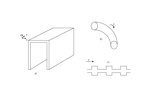
Figure 1: Examples of waveguide structures.

We study here the computation of structures considered as waveguides, as shown in figure 1, with symmetries which can be a translation (a), a rotation (b) or a periodicity (c). Thus these waveguides can be uniform or periodic. The vibration of such waveguides has been the topic of much research. One can find analytical or finite element models of waveguides and people are generally interested by the computation of wave propagations and dispersion curves or by the determination of the frequency response functions. A first approach considers structures with constant cross sections as the cases a) and b) of figure 1. For example, [1] and [2] used a wave approach to study the vibrations of structural networks composed of simple uniform beams, and solved for the dynamics of individual elements and of the junctions between elements by analytical methods. The efficiency is greatly improved compared to FE methods as a beam can be modelled using only a single element.

The first numerical approaches were proposed by [3, 4] to approximate the cross-sectional deformations by finite elements. The authors of [5, 6] applied similar ideas to the calculation of wave propagations in rails using a finite element model of the cross-section of a rail. They then calculated dispersion relations and accelerances. Dispersion relations for elastic waves in helical waveguides were also considered by [7]. For general waveguides with a complex cross-section, the displacements in the cross-section can be described by the finite element method while the variation along the axis of symmetry is expressed as a wave function. Following these ideas, [8, 9, 10, 11, 12, 13] developed the spectral finite element approach. This leads to efficient computations of dispersion relations and transfer functions but special elements need to be developed for each element type. This makes the connection with the standard use of the finite element method difficult and does not allow the benefits of powerful existing finite element software to be exploited. Similar techniques were also developed by [14, 15] for the computation of dispersion relations in damped waveguides.

More general waveguides can be studied by considering periodic structures. Numerous works provided interesting theoretical insights in the behaviour of these structures, see for instance the work of [16] and the review paper by [17]. Mead also presented a general theory for wave propagation in periodic systems in [18, 19, 20]. He showed that the solution can be decomposed into an equal number of positive and negative-going waves. The approach is mainly based on Floquet’s principle or the transfer matrix and the objective it to compute propagation constants relating the forces and displacements on the two sides of a cell (a single period) and the waves associated to these constants. For complex structures FE models are used for the computation of the propagation constants and waves. The final objective is to compute dispersion relations to use them in energetic methods, see [21, 22, 23, 24, 25]. In [26] the general dynamic stiffness matrix for a periodic structure was found from the propagation constants and waves. It leads to a matrix linking the extreme sides of the structure and allows to compute transfer functions in the structure.

The last approach is purely computational and uses rotational and cyclic symmetries to solve the problem by a decomposition of the displacements in cosine and sine functions. It is thus possible to find the transfer functions or modal shapes for periodic structures. A review of the current practises can be found in [27]. These methods allow computing the frequency response functions in a number of operations proportional to the number of cells in the structure. This paper develops this last approach and presents a recursive method to calculate the forced response of structures such as those illustrated in figure 1. A section of the waveguide is modelled using conventional FE methods, using a commercial FE package. The resulting mass, stiffness and damping matrices are then post-processed to give the dynamic stiffness matrix of the cell. Then a recursive method is applied to compute the global dynamic stiffness matrix of the whole waveguide and finally the transfer functions in the structure.

This paper presents a different approach from the previously published paper [26]. Both papers aim at computing the global dynamic stiffness matrix of a N cells structure. But in [26] waves in a period were computed and from these waves the dynamic stiffness matrix of a complete structure was obtained with a computational cost independent of the number of periods in the structure. However the computation of the waves can be time consuming when the number of dofs in a section is large because this needs the computation of eigenvalues of non symmetric matrices. On the contrary, in the present approach no wave needs to be computed and the global dynamic stiffness matrix is obtained by products and inverses of matrices with the same dimensions as the dynamic stiffness matrix of a cell. Then, the frequency response functions can be obtained easily without the computation of any wave.

The paper is divided into two parts. In the first part the recursive method for the finite element analysis of periodic structures is presented. In the second part two examples consisting in a beam and a plate are described before the conclusion.

2 Finite element analysis of periodic structures

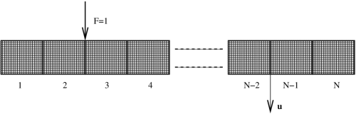
Figure 2: Periodic structure made of N cells with an excitation by a force $\mathbf{F}$.

Consider a periodic structure, as shown in figure 2, which is made of a large number $N$ of cells. We are interested by the computation of the frequency response function for a point force excitation $F=1$ somewhere in the structure and a response $u$ at another point. We propose here an efficient method to compute this function by using a recursive approach to get the dynamic stiffness matrix of different sets of cells.

2.1 Behaviour of a cell

Consider first the case of only one cell. The discrete dynamic equation of a cell obtained from a FE model at a frequency $\omega$ and for the time dependence $e^{-i\omega t}$ is given by:

$$(\mathbf{K}-i\omega\mathbf{C}-\omega^{2}\mathbf{M})\mathbf{q}=\mathbf{f}$$ (1)

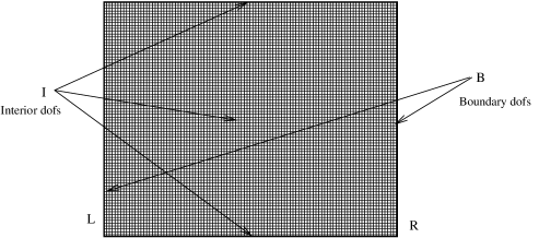
Figure 3: Interior and boundary dofs for a single cell.

where $\mathbf{K}$, $\mathbf{M}$ and $\mathbf{C}$ are the stiffness, mass and damping matrices, respectively, $\mathbf{f}$ is the loading vector and $\mathbf{q}$ the vector of the degrees of freedom (dofs). A viscous damping is considered here but the same results could be obtained with other damping models. Introducing the dynamic stiffness matrix $\widetilde{\mathbf{D}}=\mathbf{K}-i\omega\mathbf{C}-\omega^{2}\mathbf{M}$, decomposing the dofs into boundary $(B)$ and interior $(I)$ dofs as shown in figure 3, and assuming that there are no external forces on the interior nodes, result in the following equation:

$$\left[\begin{array}[]{cc}\widetilde{\mathbf{D}}_{BB}&\widetilde{\mathbf{D}}_{BI}\\ \widetilde{\mathbf{D}}_{IB}&\widetilde{\mathbf{D}}_{II}\end{array}\right]\left[\begin{array}[]{c}\mathbf{q}_{B}\\ \mathbf{q}_{I}\end{array}\right]=\left[\begin{array}[]{c}\mathbf{f}_{B}\\ \mathbf{0}\end{array}\right]$$ (2)

The interior dofs can be eliminated using the second row of equation (2), which results in

$$\mathbf{q}_{I}=-\widetilde{\mathbf{D}}_{II}^{-1}\widetilde{\mathbf{D}}_{IB}\mathbf{q}_{B}$$ (3)

The first row of equation (2) becomes

$$\mathbf{f}_{B}=\left(\widetilde{\mathbf{D}}_{BB}-\widetilde{\mathbf{D}}_{BI}\widetilde{\mathbf{D}}_{II}^{-1}\widetilde{\mathbf{D}}_{IB}\right)\mathbf{q}_{B}$$ (4)

It should be noted that only boundary dofs are considered in the following. The cell is assumed to be meshed with an equal number of nodes on their opposite sides. The boundary dofs for one cell are decomposed into left $(L)$ and right $(R)$ dofs as shown in figure 3. Thus, equation (4) is rewritten as

$$\left[\begin{array}[]{c}\mathbf{f}_{L}\\ \mathbf{f}_{R}\end{array}\right]=\left[\begin{array}[]{cc}\mathbf{D}_{LL}^{(1)}&\mathbf{D}_{LR}^{(1)}\\ \mathbf{D}_{RL}^{(1)}&\mathbf{D}_{RR}^{(1)}\\ \end{array}\right]\left[\begin{array}[]{c}\mathbf{q}_{L}\\ \mathbf{q}_{R}\end{array}\right]=\mathbf{D}^{(1)}\left[\begin{array}[]{c}\mathbf{q}_{L}\\ \mathbf{q}_{R}\end{array}\right]$$ (5)

where $\mathbf{D}^{(1)}$ is the dynamic stiffness matrix of a single cell. This matrix is symmetric if the matrices $\mathbf{K}$, $\mathbf{M}$ and $\mathbf{C}$ in relation (1) are symmetric.

2.2 Computation of reduced dynamic stiffness matrices

Consider a structure made of two cells with the respective dynamic stiffness matrices denoted by $\mathbf{A}$ and $\mathbf{B}$ as in figure 4. We propose to remove the internal degrees of freedom at the boundary between the two cells to compute the dynamic stiffness matrix, denoted $\mathbf{D}^{(2)}$, relating the degrees of freedom (dofs) in the first section of $A$ and the last section of $B$. The dynamic stiffness matrix of the substructure with two cells is computed by

$$\left[\begin{array}[]{c}\mathbf{f}_{1}\\ \mathbf{f}_{2}\\ \mathbf{f}_{3}\end{array}\right]=\left[\begin{array}[]{ccc}\mathbf{A}_{LL}&\mathbf{A}_{LR}&0\\ \mathbf{A}_{RL}&\mathbf{A}_{RR}+\mathbf{B}_{LL}&\mathbf{B}_{LR}\\ 0&\mathbf{B}_{RL}&\mathbf{B}_{RR}\\ \end{array}\right]\left[\begin{array}[]{c}\mathbf{q}_{1}\\ \mathbf{q}_{2}\\ \mathbf{q}_{3}\end{array}\right]$$ (6)

As there is no load on the interior section, one gets $\mathbf{f}_{2}=0$ and

$$\mathbf{q}_{2}=-\left(\mathbf{A}_{RR}+\mathbf{B}_{LL}\right)^{-1}\left(\mathbf{A}_{RL}\mathbf{q}_{1}+\mathbf{B}_{LR}\mathbf{q}_{3}\right)$$ (7)

The global dynamic stiffness matrix of the two cells structure is thus

$$\left[\begin{array}[]{c}\mathbf{f}_{1}\\ \mathbf{f}_{3}\end{array}\right] = \left[\begin{array}[]{cc}\mathbf{A}_{LL}-\mathbf{A}_{LR}\left(\mathbf{A}_{RR}+\mathbf{B}_{LL}\right)^{-1}\mathbf{A}_{RL}&-\mathbf{A}_{LR}\left(\mathbf{A}_{RR}+\mathbf{B}_{LL}\right)^{-1}\mathbf{B}_{LR}\\ -\mathbf{B}_{RL}\left(\mathbf{A}_{RR}+\mathbf{B}_{LL}\right)^{-1}\mathbf{A}_{RL}&\mathbf{B}_{RR}-\mathbf{B}_{RL}\left(\mathbf{A}_{RR}+\mathbf{B}_{LL}\right)^{-1}\mathbf{B}_{LR}\\ \end{array}\right]\left[\begin{array}[]{c}\mathbf{q}_{1}\\ \mathbf{q}_{3}\end{array}\right]$$ (14)

$$= \left[\begin{array}[]{ccc}\mathbf{D}_{LL}^{(2)}&\mathbf{D}_{LR}^{(2)}\\ \mathbf{D}_{RL}^{(2)}&\mathbf{D}_{RR}^{(2)}\end{array}\right]\left[\begin{array}[]{c}\mathbf{q}_{1}\\ \mathbf{q}_{3}\end{array}\right]$$ (19)

$$= \mathbf{D}^{(2)}\left[\begin{array}[]{c}\mathbf{q}_{1}\\ \mathbf{q}_{3}\end{array}\right]$$ (22)

This defines the matrix $\mathbf{D}^{(2)}$ which relates the forces and displacements dofs at the extreme sections of the two-cells structure. It can be easily checked that if the matrices $\mathbf{A}$ and $\mathbf{B}$ are symmetric, the resulting matrix $\mathbf{D}^{(2)}$ of relation (22) is also symmetric. The operation of removing the interior dofs is now denoted by $\left\{.,.\right\}$ such that we can write

$$\mathbf{D}^{(2)}=\left\{\mathbf{A},\mathbf{B}\right\}$$ (23)

2.3 Case of general structures

Consider now a structure without internal load and made of $2^{n}$ cells. We propose to recursively remove the internal degrees of freedom between adjacent cells to compute the dynamic stiffness matrix, denoted $\mathbf{D}^{(2^{n})}$, relating the degrees of freedom in sections $1$ and $2^{n}$. Consider firstly a structure with two identical cells. From the precedent analysis, one sees that its dynamic stiffness matrix is given by $\mathbf{D}^{(2)}=\left\{\mathbf{D}^{(1)},\mathbf{D}^{(1)}\right\}$. Repeating the process (see an illustration in figure 5), one gets the dynamic stiffness matrix of the structure with $2^{n}$ cells in $n$ steps by the recursive relation

$$\mathbf{D}^{(2^{n})}=\left\{\mathbf{D}^{(2^{n-1})},\mathbf{D}^{(2^{n-1})}\right\}$$ (24)

This matrix is such that

$$\left[\begin{array}[]{c}\mathbf{f}_{1}\\ \mathbf{f}_{2^{n}}\end{array}\right]=\left[\begin{array}[]{ccc}\mathbf{D}_{LL}^{(2^{n})}&\mathbf{D}_{LR}^{(2^{n})}\\ \mathbf{D}_{RL}^{(2^{n})}&\mathbf{D}_{RR}^{(2^{n})}\end{array}\right]\left[\begin{array}[]{c}\mathbf{q}_{1}\\ \mathbf{q}_{2^{n}}\end{array}\right]=\mathbf{D}^{(2^{n})}\left[\begin{array}[]{c}\mathbf{q}_{1}\\ \mathbf{q}_{2^{n}}\end{array}\right]$$ (25)

In cases where the structure is not composed of a number of cells which equals a power of two, one can modify the previous procedure using the binary representation of the total number of cells N. Consider the example where $N=11=1011_{b}$ in binary representation. One calculates first the dynamic stiffness matrix for a structure with 8 cells, then this structure is assembled with a structure made of 2 cells which has been computed during the computation of the 8 cells structure. Finally the resulting matrix is assembled with a one cell matrix. The approach can be resumed by

$$\mathbf{D}^{(11)}=\left\{\left\{\mathbf{D}^{(8)},\mathbf{D}^{(2)}\right\},\mathbf{D}^{(1)}\right\}$$ (26)

in which the matrices $\mathbf{D}^{(2^{n})}$ are computed by the method presented before. The elimination of the interior degrees of freedom gives the matrix linking the forces and displacements degrees of freedom in sections $1$ and $N$. One can notice that the final matrix is computed with a number of operations of order $\log_{2}N$, thus saving a huge number of computations when we compare to a standard approach in which all the matrices of the cells are assembled into a global matrix.

Using this method it is easy to compute the matrices for the parts of the structure respectively on the left and on the right of the force. Assembling these two matrices, applying the appropriate boundary conditions on the first and last sections, one gets the final linear system. This system has a number of dofs which equals approximately three times the number of dofs in a section.

3 Examples

3.1 Beam structure

In the first example, we consider the beam shown in figure 6 which is made of elements with four dofs. The stiffness and mass matrices of an element of length $l$ are given by

$$\mathbf{K}_{e}=\frac{EI}{l^{3}}\left[\begin{array}[]{cccc}12&6l&-12&6l\\ 6l&4l^{2}&-6l&2l^{2}\\ -12&-6l&12&-6l\\ 6l&2l^{2}&-6l&4l^{2}\end{array}\right]$$ (27)

$$\mathbf{M}_{e}=\frac{\rho Sl}{420}\left[\begin{array}[]{cccc}156&22l&54&-13l\\ 22l&4l^{2}&13l&-3l^{2}\\ 54&13l&156&-22l\\ -13l&-3l^{2}&-22l&4l^{2}\end{array}\right]$$

Here, $E$ is the Young’s modulus, $I$ the second moment of area, $\rho$ the density of the material and $S$ the cross-sectional area of the beam. Using the previous approach, one can compute the dynamic stiffness matrices for the sections on the left and on the right of the force. The damping matrix is obtained by using a complex Young modulus such that $E=E_{0}(1+i\eta)$ with $\eta=0.01$ leading to a hysteretic damping instead of the viscous one such that $\tilde{\mathbf{D}}=(1+i\eta)\mathbf{K}-\omega^{2}\mathbf{M}$. The beam is made of steal such that $E_{0}=2\times 10^{11}\mathrm{Pa}$, $\rho=7800\mathrm{kg/m^{3}}$, the length of the beam $L=1\mathrm{m}$, $I=8.33\times 10^{-14}\mathrm{m}^{4}$ and $S=10^{-6}\mathrm{m}^{2}$. The matrix for the whole beam is obtained by assembling the matrices of the left and right parts of the beam on each sides of the force. Taking into account the fixed displacement boundary conditions by removing the corresponding degrees of freedom in the global matrix results in the final system. Figure 7 presents the frequency response functions for structures with respectively 8 and 1024 elements in each part of the beam. It can be seen that 8 elements are not sufficient to compute accurately the solution while 1024 elements lead to a very good result.

In figure 8, the cpu time of the computation is plotted versus the global number of elements in the beam. The computation of 10000 points in frequency is made for each mesh of the beam and the largest mesh has $2\times 4196$ elements for the complete beam. A linear behavior of the cpu time versus the logarithm of the number of elements can be seen as expected.

3.2 Plate

Consider now the plate shown in figure 9. The mesh of a cell is obtained by Abaqus and consists in 50 elements of size $Ly/50\times Lx/2^{n}$ where $n$ is the number of cells along the direction $x$. The mass and stiffness matrices are produced by Abaqus then there are loaded in Matlab and the precedent procedure allows computing the displacement for a load at the centre of the plate. Information on the size are given in figure 9 and the plate is still made of steal. The boundary conditions are simply supported on all sides. Figure 10 presents the frequency response functions for structures with globally 32 and 512 cells. It can be seen, as for the beam, that 32 cells are not sufficient to compute accurately the solution while 512 cells lead to much better results. For high frequencies a discrepancy with the analytical solution can still be seen. It has been checked that the result can be considerably improved by taking 100 elements instead of 50 along the direction $y$. The figures also present the results from the standard finite element approach obtained by assembling the elementary matrices for each period and solving the global linear system. It can be seen that both finite elements computations yield identical results.

In figure 11, the cpu time of the computation is plotted versus the global number of cells in the plate. The computation of 100 points in frequency is made for each mesh of the plate and the largest mesh has 2048 cells along $x$ for the complete plate. Once again a linear behavior of the cpu time versus the logarithm of the number of cells can be observed. The computing times for the recursive and standard finite element methods are compared in table 1. It can be seen that the recursive method is a little slower than the standard method for a number of periods lower than 16. For a larger number of periods the recursive method tends to be more and more efficient as the number of periods increases.

4 Conclusion

A method has been described to compute frequency response functions for waveguide structures with periodic or homogeneous sections. The proposed method allows computing the solution in a time proportional to the logarithm of the numbers of cells in the structure. This simple recursive method can be applied for any type of one-dimensional periodic waveguides. It could be used in the future for the computation of complex structures such as tyres.

Figure 4: Structure with two cells and three sections.

Figure 5: Structure at each step.

Figure 6: Beam structure (a) and beam element (b).

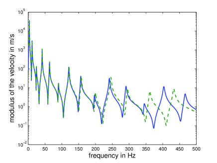
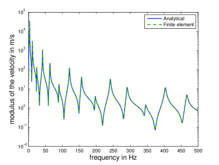
Figure 7: Frequency response functions for a beam with $2\times 8$ elements (upper graph) and $2\times 1024$ elements (lower graph): analytical solution, $---$ finite element solution. The position of the excitation point is shown in figure 6 and the response is computed at the same point.

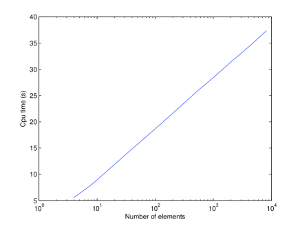
Figure 8: Computing time versus the number of cells in the beam.

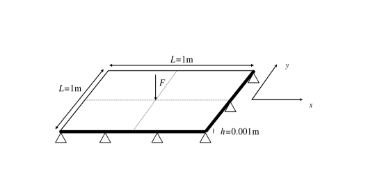
Figure 9: Plate example.

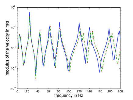
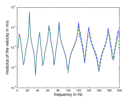
Figure 10: Frequency response functions for a plate with $2\times 16$ cells (upper graph) and $2\times 256$ cells (lower graph): analytical solution, $---$ recursive finite element solution and $.\ .$ standard finite element solution. The excitation is located at the center of the plate as shown in figure 9 and the response is computed at the same point.

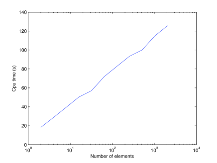
Figure 11: Computing time versus the number of cells in the plate.

Table 1: Computing times for recursive and standard FEM methods.

number of periods	recursive method (s)	classical fem (s)
2	18.3	14.4
4	28.8	20.1
8	39.5	33.7
16	50.3	69.2
32	57.0	164.3
64	71.8	435.0
128	82.7	1295.0
256	93.4	4093.1
512	100.0	13901.4
1024	114.8	49271.1
2048	125.6	184397.3

References

- [1] H. von Flotow, Disturbance propagation in structural networks, Journal of Sound and Vibration 106 (1986) 433-450.
- [2] L. S. Beale and M. L. Accorsi, Power flow in two- and three-dimensional frame structures, Journal of Sound and Vibration 185 (1995) 685-702.
- [3] S.B. Dong and R.B. Nelson, On natural vibrations and waves in laminated orthotropic plates, Journal of Applied Mechanics 39 (3) (1972) 739-745.
- [4] B. Aalami, Waves in prismatic guides of arbitrary cross section, Journal of Applied Mechanics 40 (1973) 1067-1072.
- [5] L. Gavric, Computation of propagating waves in free rail using a finite element technique, Journal of Sound and Vibration 185 (3) (1995) 531-543.
- [6] L. Gry, Dynamic modelling of railway track based on wave propagation, Journal of Sound and Vibration 195 (1996) 477-505.
- [7] F. Treyssède, Elastic waves in helical waveguides. Wave Motion 45 (4) (2008) 457-470.
- [8] S. Finnveden, Finite element techniques for the evaluation of energy flow parameters, Proc. Novem, Lyon (keynote paper), (2000).
- [9] S. Finnveden, Evaluation of modal density and group velocity by a finite element method, Journal of Sound and Vibration 273 (2004) 51-75.
- [10] C. M. Nilsson, Waveguide finite elements for thin-walled structures, Licentiate thesis, KTH, Stockholm, 2002.
- [11] F. Birgersson, S. Finnveden and C.M. Nilsson, A spectral super element for modelling of plate vibration. Part 1: general theory, Journal of Sound and Vibration 287 (2005) 297-314.
- [12] F. Birgersson and S. Finnveden, A spectral super element for modelling of plate vibration. Part 2: turbulence excitation, Journal of Sound and Vibration 287 (2005) 315-328.
- [13] S. Finnveden and M. Fraggstedt, Waveguide finite elements for curved structures, Journal of Sound and Vibration 312 (2008) 644-671.
- [14] I. Bartoli, A. Marzani, F. Lanza di Scalea and E. Viola, Modeling wave propagation in damped waveguides of arbitrary cross-section. Journal of Sound and Vibration 295 (3-5) (2006) 685-707.
- [15] A. Marzani, E. Viola, I. Bartoli, F. Lanza di Scalea and P. Rizzo, A semi-analytical finite element formulation for modeling stress wave propagation in axisymmetric damped waveguides. Journal of Sound and Vibration 318 (2008) 488-505.
- [16] L. Brillouin, Wave propagation in periodic structures. New York: Dover, 1953.
- [17] D. J. Mead, Wave propagation in continuous periodic structures: research contributions from Southampton, 1964-1995, Journal of Sound and Vibration 190 (1996) 495-524.
- [18] D. J. Mead, A general theory of harmonic wave propagation in linear periodic systems with multiple coupling, Journal of Sound and Vibration 27 (1973) 235-260.
- [19] D. J. Mead, Wave propagation and natural modes in periodic systems: I. Mono-coupled systems, Journal of Sound and Vibration 40 (1975) 1-18.
- [20] D. J. Mead, Wave propagation and natural modes in periodic systems: II. Multi-coupled systems, with and without damping, Journal of Sound and Vibration 40 (1975) 19-39.
- [21] L. Houillon, M.N. Ichchouh and L. Jezequel, Wave motion in thin-walled structures, Journal of Sound and Vibration 281 (2005) 483-507.
- [22] B. R. Mace, D. Duhamel, M. J. Brennan and L. Hinke, Wavenumber Prediction Using Finite Element Analysis. 11th International Congress on Sound and Vibration, St. Petersburg (2004).
- [23] B. R. Mace, D. Duhamel, M. J. Brennan and L. Hinke, Finite element prediction of wave motion in structural waveguides, Journal of the Acoustical Society of America 117 (2005) 2835-2843.
- [24] J.M. Mencik and M.N. Ichchou, Multi-mode propagation and diffusion in structures through finite elements, European Journal of Mechanics A/Solids 24 (2005) 877-898.
- [25] J.M. Mencik and M.N. Ichchou, Wave finite elements in guided elastodynamics with internal fluid, International Journal of Solids and Structures 44 (2007) 2148-2167.
- [26] D. Duhamel, B.R. Mace and M.J. Brennan, Finite element analysis of the vibrations of waveguides and periodic structures, Journal of Sound and Vibration 294 (2006) 205-220.
- [27] D. Wang, C. Zhou and J. Rong, Free and forced vibration of repetitive structures, International Journal of Solids and Structures 40 (2003) 5477-5494.