Interplay of anisotropy and frustration: triple transitions in a triangular-lattice antiferromagnet

Abstract

The classical Heisenberg antiferromagnet on a triangular lattice with the single-ion anisotropy of the easy-axis type is studied theoretically. The phase diagram in an external magnetic field is constructed from the mean-field analysis. Three successive Berezinskii-Kosterlitz-Thouless transitions are found by Monte Carlo simulations in zero field. Two upper transitions are related to the breaking of the discrete $\mathbb{Z}_{6}$-symmetry, while the lowest transition is associated with a quasi-long-range ordering of transverse components. The intermediate collinear phase between the first and second transition is the critical phase predicted by J. V. José et al. [Phys. Rev. B 16, 1217 (1977)].

I Introduction

Frustrated magnetic systems have been a stimulating research topic over several decades. Their diverse properties, highly degenerate ground states, non-collinear ordering, novel phase transitions,Diep2005 offer a playground to investigate fundamental physical questions going far beyond magnetism itself. One of the specific subjects in this field is the interplay of geometrical frustration and magnetic anisotropies. The prominent example is provided by the rare-earth pyrochlore materials with Ising-type magnetic moments. Contrary to naive expectations, these magnetic systems remain non-frustrated for an antiferromagnetic nearest-neighbor coupling, but develop highly frustrated spin-ice states for the case of a ferromagnetic exchange between spins.Harris97 ; Moessner98 ; Ramirez99

In the present work we investigate the nearest-neighbor Heisenberg antiferromagnet on a triangular lattice with the single-ion anisotropy of the easy-axis type:

$${\cal H}=J\sum_{\langle ij\rangle}{\bf S}_{i}\cdot{\bf S}_{j}-D\sum_{i}(S^{z}_{i})^{2}$$ (1)

Such a Hamiltonian is believed to describe quasi two-dimensional (2D) magnetic materials ${\rm VCl_{2}}$ (Ref. Kadowaki87, ) and ${\rm LiCrO_{2}}$ (Ref. Kadowaki95, ). A similar model with the $XXZ$ anisotropy has been previously studied by a number of authors.Miyashita85 ; Sheng92 ; Stephan00 In real magnetic materials with $S>\frac{1}{2}$ the single-ion anisotropy being the first-order relativistic effect is usually more significant than the anisotropic exchange, which is generally of the second-order in the spin-orbital coupling. Yosida96 Besides, as we shall see later, the two types of anisotropy lead to different sequences of finite-temperature phase transitions.

Ordered states of the anisotropic triangular antiferromagnet (1) are characterized by a nonzero static magnetization:

$$\langle{\bf S}_{i}\rangle={\bf l}_{1}\cos({\bf Q}\cdot{\bf r}_{i})+{\bf l}_{2}\sin({\bf Q}\cdot{\bf r}_{i})+{\bf m}\ .$$ (2)

with the ordering wave vector ${\bf Q}=(4\pi/3,0)$. At zero temperature the Heisenberg triangular-lattice antiferromagnet orders in a three-sublattice $120^{\circ}$ spin structure. Such a noncollinear magnetic ordering is described by a pair of orthogonal antiferromagnetic vectors: ${\bf l}_{1}\perp{\bf l}_{2}$, $|{\bf l}_{1}|=|{\bf l}_{2}|$, and ${\bf m}\equiv 0$. In accordance with the Mermin-Wagner theorem there is no symmetry breaking transition at any finite temperature. Still a weak topological transition related to proliferation of $\mathbb{Z}_{2}$-vortices may occur for this model at $T/J\sim 0.3$.Kawamura84 ; Wintel94 ; Southern95 ; Caffarel01 ; Kawamura07 For the easy-plane anisotropy, $D<0$ in Eq. (1), the spin plane of the ordered $120^{\circ}$ structure is fixed to the $x$–$y$ plane. In this case two finite temperature transitions take place: the Ising-type transition related to the chiral symmetry breaking and the Berezinskii-Kosterlitz-Thouless (BKT) transition associated with the vortex-antivortex unbinding.Capriotti98

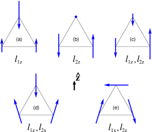
Figure 1: (Color online) Possible three-sublattice planar configurations of the easy-axis triangular antiferromagnet. The direction of the easy-axis is shown by ${\bf\hat{z}}$. The nonzero components of the order parameter (2) are indicated for each configuration.

The easy-axis anisotropy, $D>0$, orients the spin plane perpendicular to the $x$–$y$ crystallographic plane and simultaneously distorts the spin structure. Finding directions and magnitudes of ${\bf l}_{1}$ and ${\bf l}_{2}$ becomes a nontrivial problem in this case. Possible spin structures corresponding to the ordering wave vector ${\bf Q}$ are presented in Fig. 1. They have been obtained by a symmetry analysis and are confirmed by the mean-field calculations described in the next section. Some of these states, Figs. 1(a), (c), and (d), have a finite uniform magnetization $\bf m$ along $\hat{\bf z}$, which is, however, a secondary order parameter and not indicated for that reason in the Figure.

In order to elucidate symmetries of different phases, we note that a simple translation $\hat{T}_{\bf a}$ (${\bf r}_{i}\rightarrow{\bf r}_{i}+{\bf a}$) transforms the antiferromagnetic order parameter according to

$$\hat{T}_{\bf a}\bigl{[}({\bf l}_{1}+i{\bf l}_{2})\bigr{]}=({\bf l}_{1}+i{\bf l}_{2})\;e^{-i{\bf Q}\cdot{\bf a}}\ ,$$ (3)

where the phase factor can take only three different values: ${\bf Q}\cdot{\bf a}=0,\pm 2\pi/3$. Hence, besides the group $S_{1}$ of continuous rotations about the $\hat{\bf z}$-axis the magnetic structure has an inherent discrete symmetry $\mathbb{Z}_{3}$. Such an additional symmetry corresponds to permutations of three sublattices. In zero magnetic field the time-reversal symmetry implies invariance with respect to ${\bf l}_{i}\rightarrow-{\bf l}_{i}$, which enlarges $\mathbb{Z}_{3}$ to $\mathbb{Z}_{6}$. The total symmetry group is, therefore,

$$G=S_{1}\otimes\mathbb{Z}_{6}\ ,$$ (4)

see also a similar discussion in Ref. Sheng92, . The collinear phases shown in Figs. 1(a)-(c) preserve the axial symmetry $S_{1}$ but break in different ways the discrete symmetry group $\mathbb{Z}_{6}$. In terms of the order parameter angle $\varphi$ defined by

$$l_{1z}=l\cos\varphi\ ,\qquad l_{2z}=l\sin\varphi\ ,$$ (5)

the state in Fig. 1(a) corresponds to commensurate values $\varphi=2k\pi/6$ with an integer $k$, whereas the configuration in Fig. 1(b) has $\varphi=(2k+1)\pi/6$. The third type of a collinear state is described by an arbitrary angle $\varphi$ and is shown schematically in Fig. 1(c). In such a state the phase $\varphi$ remains unlocked and the sine and cosine harmonic (5) coexist with an arbitrary ratio.

For large enough values of $D/J>d_{c}=1.5$ the magnetic anisotropy induces a highly degenerate collinear Ising state at zero temperature. Quantum fluctuations can lead, then, to interesting zero- and finite-temperature phases.Damle07 ; Sen09 Here, we investigate an antiferromagnet with a moderate-strength anisotropy $0<D/J<d_{c}$, which is frequently found among experimental systems, and consider the finite-temperature properties of the model (1). For simplicity, we neglect quantum effects and study the classical spin model.

Layered easy-axis triangular antiferromagnets with a significant interplane coupling exhibit two second-order transitions with an intermediate collinear $l_{1}$-phase shown in Fig. 1(a).Plumer88 In contrast, we show in the present work that a purely 2D system (1) shows three consecutive BKT-type transitions. In the first part, Sec. II, we investigate the mean-field phase diagram of the model (1) at zero and at finite magnetic fields. The mean-field behavior is expected to be realized in layered triangular antiferromagnets with weak interplane coupling. The Monte Carlo (MC) simulations and the analysis of the zero-field behavior of the model (1) are presented in the second part of our study, Sec. III.

II Mean-field theory

Let us begin with the mean-field analysis of possible finite-temperature phases of the model (1). Specifically, we use the real-space approach,Bak80 ; Suzuki83 ; Cepas04 ; Enjalran04 generalizing the previously established technique to systems with the single-ion anisotropy. The two standard steps of the mean-field approximation include (i) decoupling the spin-spin interaction according to

$${\bf S}_{i}\cdot{\bf S}_{j}\approx{\bf S}_{i}\cdot\langle{\bf S}_{j}\rangle+\langle{\bf S}_{i}\rangle\cdot{\bf S}_{j}-\langle{\bf S}_{i}\rangle\cdot\langle{\bf S}_{j}\rangle\ ,$$ (6)

with $\langle{\bf S}_{i}\rangle$ being the thermal average of an $i^{\rm th}$ magnetic moment and (ii) rewriting ${\cal H}$ as a sum of single-site Hamiltonians

$${\cal H}_{\rm MF} = \sum_{i}\big{[}-D(S^{z}_{i})^{2}-{\bf h}_{i}\cdot{\bf S}_{i}\big{]}-J\sum_{\langle ij\rangle}\langle{\bf S}_{i}\rangle\cdot\langle{\bf S}_{j}\rangle$$ (7)

$${\rm with}\ \ \ {\bf h}_{i}={\bf H}-J\sum_{\rm n.n.}\,\langle{\bf S}_{j}\rangle\ ,$$

where we have also added a Zeeman magnetic field to Eq. (1). Due to the presence of the single-ion term in ${\cal H}_{\rm MF}$, the local magnetization $\langle{\bf S}_{i}\rangle$ has to be decomposed into components, which are transverse and parallel to the anisotropy axis:

$$\langle{\bf S}_{i}\rangle=\langle S^{z}_{i}\rangle\,{\bf{\hat{z}}}+\langle S^{\perp}_{i}\rangle\,\frac{[{\bf h}_{i}-h_{i}^{z}{\bf{\hat{z}}}]}{h_{i}^{\perp}}\ .$$ (8)

Performing integration with respect to $x=S^{z}_{i}=\cos\theta_{i}$ in the expression for the partition function we obtain the following mean-field equations for static magnetic moments:

$$\langle S_{i}^{\perp}\rangle = \frac{1}{2Z_{i}}\int_{-1}^{1}\mathrm{d}x\,\sqrt{1-x^{2}}\,e^{Dx^{2}/T}\,e^{h_{i}^{z}x/T}I_{1}(y_{i})\ ,$$

$$\langle S_{i}^{z}\rangle = \frac{1}{2Z_{i}}\int_{-1}^{1}\mathrm{d}x\,x\,e^{Dx^{2}/T}\,e^{h_{i}^{z}x/T}\;I_{0}(y_{i})\ ,$$ (9)

$$Z_{i} = \frac{1}{2}\int_{-1}^{1}\mathrm{d}x\;e^{Dx^{2}/T}\>e^{h_{i}^{z}x/T}I_{0}(y_{i})\ ,$$

where $y_{i}=h_{i}^{\perp}\sqrt{1-x^{2}}/T$ and $I_{n}(z)$ is the modified Bessel function of the $n$-th order:

$$I_{n}(z)=\frac{1}{\pi}\int_{0}^{\pi}\mathrm{d}\alpha\,e^{z\cos\alpha}\,\cos^{n}\!\alpha\ .$$

The system of integral equations (9) together with the self-consistency condition given by Eq. (7) is solved iteratively on finite lattices of $N=L\times L$ spins, with periodic boundary conditions. Once convergence is achieved, various physical quantities are calculated including the free-energy

$${\cal F}_{\rm MF}=-J\sum_{\langle ij\rangle}\langle{\bf S}_{i}\rangle\cdot\langle{\bf S}_{j}\rangle-T\sum_{i}\ln Z_{i}\ ,$$ (10)

the internal energy $E_{\rm MF}=\langle{\cal H}_{\rm MF}\rangle$, and the antiferromagnetic order parameters. By explicit calculations for clusters with $3\leq L\leq 12$ at all temperatures and weak magnetic fields we have verified stability of the three-sublattice structure with ${\bf Q}=(4\pi/3,0)$. After that a more detailed investigation of the $H$–$T$ phase diagram has been performed with the three-sublattice ansatz. Precise location of phase boundaries in Fig. 2 has been determined from temperature and field scans for the antiferromagnetic order parameters indicated in Fig. 1 as well as for the uniform magnetization. The behavior of the specific heat has been also used to independently verify these results.

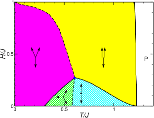
Figure 2: (Color online) The low-field part of the mean-field phase diagram with ${\bf H}\parallel\hat{\bf z}$ for a representative value $D/J=1$. Spin configurations for each phase are schematically indicated by arrows as in Fig. 1. Solid and dashed lines correspond to first- and second-order transitions, respectively.

At the upper transition $T_{c1}\simeq 1.2J$ in zero magnetic field only $z$-components of magnetic moments become ordered. In accordance with the $\mathbb{Z}_{6}$ symmetry selection between various collinear structures is determined by the following invariant in the Landau free-energy:

$$A_{6}\bigl{[}(l_{1}^{z}+il_{2}^{z})^{6}+\textrm{c.\,c.}\bigr{]}\ .$$ (11)

For negative $A_{6}<0$ the pure $l_{1}$-state, Fig. 1(a), is energetically favored, while $A_{6}>0$ corresponds to the $l_{2}$-state, Fig. 1(b). We have verified the positive sign of $A_{6}$ in our case by a direct analytical expansion of Eqs. (9). Our numerical results also confirm that the $l_{2}$-state is stable below $T_{c1}$. Such a partially ordered phase has a vanishing moment on one of the antiferromagnetic sublattices. A similar phase has been discussed in relation to the intriguing phase diagram of ${\rm Gd_{2}Ti_{2}O_{7}}$.Stewart04 Here, we provide an example, where a partially ordered phase is realized at the mean-field level in a simple spin model.

The second transition at $T_{c2}\simeq 0.6J$ is related to the breaking of the rotational symmetry about $\hat{\bf z}$-axis. Below $T_{c2}$ the third previously disordered magnetic sublattice becomes ordered with moments oriented within the $x$–$y$ plane. Simultaneously, moments of the other two sublattices start deviating from $\hat{\bf z}$-axis leading to a distorted triangular structure shown in Fig. 1(e). This distorted spin structure is characterized by ${\bf l}_{2}\parallel\hat{\bf z}$ and ${\bf l}_{1}\perp{\bf l}_{2}$. When temperature is further decreased the coefficient $A_{6}$ in the effective anisotropy term changes sign at $T_{c3}\simeq 0.3$ and one finds a first-order transition into another distorted triangular structure shown in Fig. 1(d) with ${\bf l}_{1}\parallel\hat{\bf z}$.

Note, that the related model with the exchange anisotropy Miyashita85 ; Sheng92 has $A_{6}=0$ in the mean-field approximation, which leads to an additional continuous degeneracy. As a result, only two finite-temperature transitions are found in this case: from the paramagnetic state to a degenerate collinear configuration shown in Fig. 1(c) and then to a degenerate distorted $120^{\circ}$ configuration.Miyashita85 ; Stephan00 Sheng and Henley Sheng92 have discussed how different types of fluctuations, thermal, quantum, or random dilution, can induce a finite $A_{6}$. For the model with the single-ion anisotropy one finds a different interesting possibility: the sign of the anisotropic term changes upon lowering temperature.

The two phases in Figs. 1(a) and (d) have a nonvanishing total magnetization $m^{z}$. The coupling between ferro- and antiferromagnetic components is determined by the term

$$m^{z}(l_{1}^{z}+il_{2}^{z})^{3}+\textrm{c.\,c.}\ ,$$ (12)

which is invariant under $\mathbb{Z}_{3}$ transformations (3). In zero magnetic field this yields $m^{z}\sim(T_{c}-T)^{3/2}$ for states with ${\bf l}_{1}\parallel\hat{\bf z}$. In contrast, states in Fig. 1(b) and 1(e) with ${\bf l}_{2}\parallel\hat{\bf z}$ have vanishing $m^{z}$. This difference is important to understand the finite-field behavior, see Fig. 2. Magnetic field applied parallel to the $\hat{{\bf z}}$-axis favors spin structures with a finite magnetization and stabilizes states with $l_{1}^{z}\neq 0$, which is why the two intermediate low-field phases are no longer pure $l_{2}^{z}$ states. This feature is emphasized by hatches in Fig. 2. The collinear-noncollinear transitions are of the second order, whereas all other transition lines are of the first order. In the case of the transition from the paramagnetic state in external magnetic field the first-order nature of the transition follows from the presence of the cubic invariant (12), while in other cases the above conclusion is a consequence of the group-subgroup relation. The transition lines intersect at a multicritical point $(T^{*},H^{*})=(0.6J,0.25J)$.

The mean-field phases and the structure of the phase diagram at fields larger than $H^{*}$ are similar to the Heisenberg triangular antiferromagnet Kawamura85 so we do not go into further details. We have also checked other moderate values of $D/J<1.5$ and found precisely the same structure of stable phases with triple transitions in zero magnetic field. As we shall see in the next section, the true thermodynamic phases determined by Monte Carlo simulations of the model (1) differ from the mean-field solutions, which is often the case in 2D. Still, the mean-field picture is expected to be qualitatively correct for 3D layered triangular antiferromagnets. By including a ferro- or antiferromagnetic interlayer coupling $J^{\prime}$ in the mean-field equations (7) and (9) we have verified that the predicted sequence of finite-temperature transitions remains valid up to $|J^{\prime}/J|\sim 0.6$. For larger values of $|J^{\prime}/J|$ we find a double transition with an intermediate $l_{1}$ collinear phase similar to the previously studied case of very strong $J^{\prime}$.Plumer88

III Monte Carlo simulation

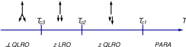
Figure 3: Schematic zero-field phase diagram of the two-dimensional triangular antiferromagnet with easy-axis single-ion anisotropy. The arrow labeling of phases is the same as in Fig. 1.

In uniaxial magnetic systems, transverse and longitudinal spin components order at different temperatures as they belong to different irreducible representations. For the triangular antiferromagnet with the easy-axis anisotropy, the highest transition should be related to the sole breaking of $\mathbb{Z}_{6}$ symmetry. Such a discrete symmetry breaking may lead to a phase with a true long-range ordering at low temperatures even in 2D. The case of a 2D system with the general $\mathbb{Z}_{p}$ symmetry has been considered in the seminal work of José and co-workers.JKKN77 The precise nature and sequence of finite-temperature transitions depend on the number $p$ of “clock states.” José et al. have predicted two BKT-type transitions for $p=6$. A massive phase with a true long-range order appears below the lower transition at $T_{c2}$, while at intermediate temperatures $T_{c2}<T<T_{c1}$ a gapless phase with an algebraic quasi long-range order is realized. In our case the massive phase is represented by one of the states in Figs. 1(a) and (b), while the gapless phase correspond to a state in Fig. 1(c) with a power law decay of spin-spin correlations:

$$\langle S_{i}^{z}S_{j}^{z}\rangle\sim\frac{\cos({\bf Q}\cdot{\bf r}_{ij})}{r_{ij}^{\eta}}\ .$$ (13)

The critical exponent $\eta$ continuously varies from $\eta_{1}=1/4$ at $T=T_{c1}$ to $\eta_{2}=1/9$ at $T=T_{c2}$. The subsequent BKT transition related to the appearance of quasi-long-range order in the transverse components is expected to occur at an independent transition temperature $T_{c3}<T_{c1}$. The expected sequence of finite-temperature phases is schematically shown in Fig. 3 with three BKT-type transitions. A similar suggestion was made before for the triangular antiferromagnet with the exchange anisotropy, Sheng92 though no supporting numerical results were presented.

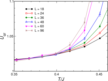
Figure 4: (Color online) Temperature dependence of the Binder cumulant for the antiferromagnetic order parameter $m_{\bf Q}^{z}$ for different cluster sizes.

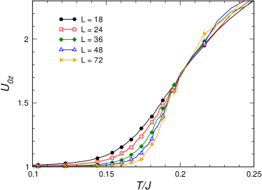
Figure 5: (Color online) Temperature dependence of the Binder cumulant for the uniform magnetization $m_{z}$ for different cluster sizes.

To verify the outlined scenario in our case we have performed Monte Carlo simulations of the model (1) in zero magnetic field for the same value of the anisotropy parameter $D/J=1$ as in Sec. II. Rhombic lattice clusters with periodic boundary conditions and with $N=L^{2}$ sites, $L=18-96$, have been studied using the standard Metropolis algorithm. Restricted motion of spins was implemented at low temperatures to keep the acceptance rate around $50\%$. In order to improve further the performance of the MC algorithm, we have added a few microcanonical over-relaxation steps.Creutz87 ; Kanki05 For models without the single-ion term an over-relaxation move consists in a random rotation of a given spin about the local magnetic field. Such a step would not conserve the single-ion energy in (1). We choose, therefore, to reflect a spin with respect to the plane ${\bf n}$–${\bf h}$, where ${\bf n}$ is the anisotropy axis and ${\bf h}$ is the local field. In total $2\cdot 10^{6}$ hybrid MC steps were used at each temperature and results were further averaged over 20 different cooling runs, which both reduces measurement noise and provides an unbiased estimate of the statistical errors.

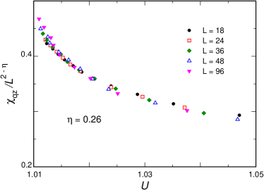
Figure 6: (Color online) Scaling plot for the normalized susceptibility versus the Binder cumulant in the vicinity of the upper transition $T_{c1}$. The indicated value of the exponent $\eta$ is used to achieve the best collapse of data from different clusters.

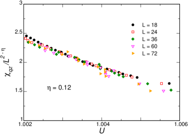
Figure 7: (Color online) Scaling plot for the normalized susceptibility versus the Binder cumulant in the vicinity of the second transition $T_{c2}$. The indicated value of the exponent $\eta$ is used to achieve the best collapse of data from different clusters.

The standard technique to locate a BKT transition is to measure the spin stiffness, Ohta79 ; Teitel83 ; Weber88 ; Chaikin00 which jumps from zero to the universal value $\rho_{s}=2T_{\rm BKT}/\pi$. However, in the case of an underlying discrete symmetry definition of $\rho_{s}$ becomes problematic. Therefore, we initially focus on the behavior of the Binder cumulant $U_{A}=\langle A^{4}\rangle/\langle A^{2}\rangle^{2}$, where $A$ is the appropriate order parameter given by Eq. (14) below. When correlations of the considered order parameter are critical the value of the Binder cumulant becomes size-independent. As a result, the curves $U_{L}(T)$ measured for different cluster sizes $L$ cross at the same point for a second-order transition, whereas for a BKT transition they merge once the correlation length is infinite. Loison99

At every temperature we have separately measured even powers of different components of the order parameter

$$(m_{{\bf q}}^{\alpha})^{2}=\frac{1}{N^{2}}\sum_{i,j}\langle S_{i}^{\alpha}S_{j}^{\alpha}\rangle\,e^{i{\bf q}({\bf r}_{i}-{\bf r}_{j})}$$ (14)

for $\alpha=z$ and $x,y$ and for ${\bf q}={\bf Q},0$. Numerical results for $z$-components are presented in Figs. 4 and 5, which allow to locate approximately $T_{c1}/J\sim 0.4$ and $T_{c2}/J\sim 0.2$. For the second transition we use for illustration the uniform magnetization $m^{z}$ instead of $m_{\bf Q}^{z}$. Nonzero values of $m^{z}$ unambiguously establish $l_{1}$-state in Fig. 1(a) as the low-temperature state with the broken $\mathbb{Z}_{6}$ symmetry. In addition, this choice yields less noisy results. Still, statistical errors are significant and the precise location of the transition point is difficult with this method.

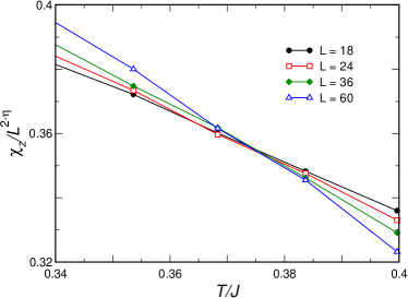
Figure 8: (Color online) Temperature dependence of the normalized susceptibility with $\eta=1/4$ for different cluster sizes in the vicinity of the upper transition. The common crossing point yields $T_{c1}/J\approx 0.377$.

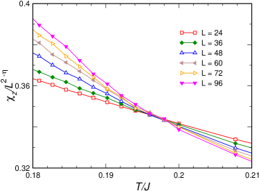
Figure 9: (Color online) Temperature dependence of the normalized susceptibility with $\eta=1/9$ for different cluster sizes in the vicinity of the lower transition. The common crossing point yields $T_{c2}/J\approx 0.198$.

The renormalization group prediction JKKN77 for the exponent $\eta$ in the vicinity of the two transitions can be, however, tested without precise knowledge of the corresponding $T_{c}$. Loison99 In the critical regime the general scaling law Barber83 reads as

$$U_{L}(T)=f(L/\xi)\quad\mathrm{and}\quad\chi=L^{2-\eta}g(L/\xi)\ ,$$ (15)

where $\chi=L^{2}m^{2}_{{\bf q}\alpha}/T$ is the generalized susceptibility, and $\xi$ is the correlation length. Hence, the plot of $\chi/L^{2-\eta}$ against $U_{L}$ for the correct value of $\eta$ should exhibit a collapse of numerical data for different cluster sizes onto a single curve. Figures 6 and 7 show the best fits around $T_{c1}$ and $T_{c2}$ respectively, which yield $\eta_{1}=0.26\pm 0.01$ and $\eta_{2}=0.12\pm 0.01$. The obtained values are in a very good agreement with the prediction $\eta_{1}=1/4$ and $\eta_{2}=1/9$. JKKN77

Once the value of the critical exponent $\eta$ is precisely established, one can use it to accurately estimate the transition temperature from the finite-size scaling of susceptibility (15). Cuccoli95 ; Wysin05 The curves $\chi/L^{2-\eta}$ for different cluster sizes shown in Figs. 8 and 9 exhibit very tight crossing points giving us the following estimates for the transition temperatures: $T_{c1}/J=0.377\pm 0.001$ and $T_{c2}/J=0.198\pm 0.001$.

The third BKT transition, which corresponds to a quasi-long-range ordering of transverse components, occurs at $T_{c3}<T_{c2}$. To precisely locate $T_{c3}$ we measure the spin stiffness. The spin stiffness $\rho_{s}$ is defined as a general elasticity coefficient in response to a weak nonuniform twist of spins $\delta\phi^{\alpha}({\bf r})$ performed about a certain direction $\alpha$ in spin space. Generally, the spin stiffness is a fourth-rank tensor with the first pair of indexes running over the spin components and the second pair spanning over the gradient components in real space. In our case it is sufficient to consider only twists about the $\hat{\bf z}$-axis in the spin space, while all directions in the lattice plane are equivalent due to the six-fold rotational symmetry. This leaves us a single parameter:

$$\delta F=\frac{\rho_{s}}{2}\int\mathrm{d}^{2}r\bigl{[}\nabla\phi^{z}({\bf r})\bigr{]}^{2}\ .$$ (16)

Choosing a twist with a uniform gradient along an arbitrary direction $\hat{\bf e}$ in the lattice plane, one obtains in spherical coordinates

$${\bf S}_{i}\cdot{\bf S}_{j} = \cos\theta_{i}\cos\theta_{j}+\sin\theta_{i}\sin\theta_{j}\cos({\tilde{\varphi}_{i}}-{\tilde{\varphi}_{j}})$$ (17)

$${\rm with}\ \ \ {\tilde{\varphi}_{i}}=\varphi_{i}+\delta\phi\,{\bf{\hat{e}}}\cdot{\bf r}_{i}\ .$$

Calculating the change of the free-energy up to the second order in a small $\delta\phi$ and normalizing result per unit area one obtains Ohta79 ; Teitel83 ; Weber88

$$\rho_{s} = -\frac{J}{N\sqrt{3}}\,\sum_{\langle i,j\rangle}\,\langle(S_{i}^{x}S_{j}^{x}+S_{i}^{y}S_{j}^{y})\rangle$$

$$\mbox{}+\frac{2J^{2}}{NT\sqrt{3}}\Bigl{\langle}\Bigl{\{}\sum_{\langle i,j\rangle}(S_{i}^{x}S_{j}^{y}\!-\!S_{i}^{y}S_{j}^{x})[\hat{\bf e}\cdot({\bf r}_{i}-{\bf r}_{j})]\Bigr{\}}^{2}\Bigr{\rangle}\ .$$

The first term in the above equation has been averaged over $\hat{\bf e}=\hat{\bf x}$ and $\hat{\bf y}$ directions. Numerical results from our MC simulations are presented in Fig. 10. We determine crossing points of $\rho^{L}_{s}(T)$ with the straight line $\rho_{s}=2T/\pi$ for each cluster size $L$ and extrapolate them to $L\rightarrow\infty$ according to $T_{\rm cross}(L)=T_{c3}+a/L$. This yields the BKT transition at $T_{c3}/J=0.168\pm 0.001$ as illustrated in the inset of Fig. 10. We have also determined the critical exponent $\eta_{3}=0.28\pm 0.03$, which coincides within the error bars with the BKT value $\eta=1/4$.

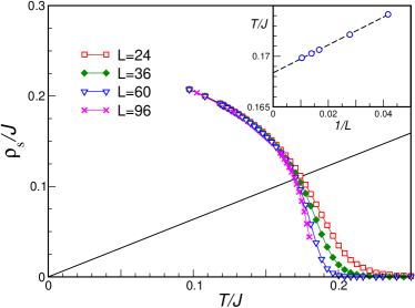
Figure 10: (Color online) The spin stiffness of the easy-axis triangular antiferromagnet for different cluster size. Intersection points with the line $\rho_{s}/T=2/\pi$ are used to locate the transition temperature. The inset presents the interpolation of the crossing points to the thermodynamic limit.

IV Summary

We have studied a simple model of the Heisenberg triangular-lattice antiferromagnet with the single-ion anisotropy of the easy-axis type. Despite its simplicity such a 2D spin model exhibits a sequence of three BKT-type transitions illustrating nontrivial physical effects which appear due to the competition between magnetic anisotropy and geometrical frustration. The Monte Carlo simulations yield for $D=J$: $T_{c1}/J=0.377$, $T_{c2}/J=0.198$, and $T_{c3}/J=0.168$. The two upper transitions correspond to the breaking of the discrete $\mathbb{Z}_{6}$ symmetry, whereas the lowest one is the standard topological transition related to the proliferation of $XY$ vortices. At $T_{c2}<T<T_{c1}$ the longitudinal spin correlations have a power law decay with distance with a continuously varying exponent $\eta$.

A remaining question is the fate of the intermediate critical phase at finite magnetic fields. An external field applied parallel to the anisotropy axis reduces the discrete symmetry from $\mathbb{Z}_{6}$ to $\mathbb{Z}_{3}$. According to José et al.,JKKN77 the $p=3$ clock model has no critical phase but exhibits instead a single transition into a normally ordered state, e.g., the phase in Fig. 1(a). It would be interesting to verify numerically the nature of this phase transition, which may be a critical one belonging to the three-state Potts model universality class JKKN77 or be of the first order due to a presence of the cubic term (12).

The mean-field calculations find the partially ordered collinear phase, Fig. 1(b), which appears to be unstable in 2D due to enhanced thermal fluctuations. Another interesting question for the future studies is whether the partially ordered state can be stabilized in layered triangular antiferromagnets. The thermal fluctuations are suppressed in this case by 3D effects, while the mean-field calculations predict stability of the partially disordered phase up to $J_{\perp}\sim 0.6J$.

References

- (1) Frustrated spin systems, ed. H. T. Diep (World Scientific, 2005).
- (2) M. J. Harris, S. T. Bramwell, D. F. McMorrow, T. Zeiske, and K. W. Godfrey, Phys. Rev. Lett. 79, 2554 (1997).
- (3) R. Moessner, Phys. Rev. B 57, R5587 (1998).
- (4) A. P. Ramirez, A. Hayashi, R. J. Cava, R. Siddharthan, and B. S. Shastry, Nature 399, 333 (1999).
- (5) H. Kadowaki, K. Ubukoshi, K. Hirokawa, J. L. Martinez, and G. Shirane, J. Phys. Soc. Jpn. 56, 4027 (1987).
- (6) H. Kadowaki, H. Takei, and K. Motoya, J. Phys.: Condens. Matter 7, 6869 (1995).
- (7) S. Miyashita and H. Kawamura, J. Phys. Soc. Jpn. 54, 3385 (1985).
- (8) Q. Sheng and C. L. Henley, J. Phys.: Condens. Matter 4, 2937 (1992).
- (9) W. Stephan and B. W. Southern, Phys. Rev. B 61, 11514 (2000).
- (10) K. Yosida, Theory of magnetism (Springer Verlag, 1996).
- (11) H. Kawamura and S. Miyashita, J. Phys. Soc. Jpn. 53, 4138 (1984).
- (12) M. Wintel, H. U. Everts, and W. Apel, Europhys. Lett. 25, 711 (1994); Phys. Rev. B 52, 13480 (1995).
- (13) B. W. Southern and H.-J. Xu, Phys. Rev. B 52, R3836 (1995).
- (14) M. Caffarel, P. Azaria, B. Delamotte, and D. Mouhanna, Phys. Rev. B 64, 014412 (2001).
- (15) H. Kawamura and A. Yamamoto, J. Phys. Soc. Jpn. 76, 073704 (2007).
- (16) L. Capriotti, R. Vaia, A. Cuccoli, and V. Tognetti, Phys. Rev. B 58, 273 (1998).
- (17) K. Damle, Physica A384, 28 (2007); A. Sen, F. Wang, and K. Damle, arXiv:0805.2658.
- (18) A. Sen, F. Wang, K. Damle, and R. Moessner, Phys. Rev. Lett. 102, 227001 (2009).
- (19) M. L. Plumer, K. Hood, and A. Caillé, Phys. Rev. Lett. 60, 45 (1988).
- (20) P. Bak and J. von Boehm, Phys. Rev. B 21, 5297 (1980).
- (21) N. Suzuki, J. Phys. Soc. Jpn. 52, 3199 (1983).
- (22) O. Cepas and B. S. Shastry, Phys. Rev. B 69, 184402 (2004).
- (23) M. Enjalran and M. J. P. Gingras, Phys. Rev. B 70, 174426 (2004).
- (24) J. R. Stewart, G. Ehlers, A. S. Wills, S. T. Bramwell and J. S. Gardner, J. Phys.: Condens. Matter 16, L321 (2004).
- (25) H. Kawamura and S. Miyashita, J. Phys. Soc. Jpn. 55, 4530 (1985).
- (26) J. V. José, L. P. Kadanoff, S. Kirkpatrick, and D. R. Nelson, Phys. Rev. B 16, 1217 (1977).
- (27) M. Creutz, Phys. Rev. D 36, 515 (1987).
- (28) K. Kanki, D. Loison, and K.-D. Schotte, Eur. Phys. J. B 44, 309 (2005); J. Phys. Soc. Jpn. 75, 015001 (2006).
- (29) T. Ohta and D. Jasnow, Phys. Rev. B 20, 139 (1979).
- (30) S. Teitel and C. Jayaparkash, Phys. Rev. B 27, 598 (1983).
- (31) H. Weber and P. Minnhagen, Phys. Rev. B 37, 5986 (1988).
- (32) P. M. Chaikin and T. C. Lubensky Principles of condensed matter physics, (Cambridge University Press, 2000).
- (33) D. Loison, J. Phys.: Condens. Matt. 11, L401 (1999).
- (34) M. N. Barber in Phase transitions and critical phenomena, ed. C. Domb and J. L. Lebowitz (Academic Press, 1983).
- (35) A. Cuccoli, V. Tognetti, and R. Vaia, Phys. Rev. B 52, 10221 (1995).
- (36) G. M. Wysin, Phys. Rev. B 71, 094423 (2005).