Axial Vector Coupling and Chiral Anomaly in the Spectral Quark Model

Abstract

We studied the Adler-Bardeen-Bell-Jackiw anomaly in the context of a finite chiral quark model known as the Spectral Quark Model. Within this model, we obtain the general non-local form of the axial vertex compatible with a non vanishing axial coupling, in the chiral limit. The triangle anomaly is computed and we show that the obtained dependence of the axial vertex with the spectral mass is necessary to ensure both finiteness and the correct violation of the chiral Ward-Takahashi identity.

I Introduction

The non-perturbative low energy behavior of Quantum Chromodynamics (QCD) is well described by a series of effective models Gell-Mann and L’evy (1960); Nambu and Jona-Lasinio (1961a, b) in both zero and finite temperature and densities Ram Mohan (1976); Asakawa and Yazaki (1989); Klimt et al. (1990); Kunihiro (1991); Caldas (2004); Caldas and Nemes (2001); Caldas et al. (2001, 1997); Andersen et al. (2004); Andersen and Brauner (2008); Petropoulos (1999); Roh and Matsui (1998); Goldberg (1983); Lenaghan et al. (2000); Baym and Grinstein (1977); Reinhardt and Dang (1987); Christov et al. (1991); Ebert et al. (1993); Schwarz et al. (1999). It is assumed that these models could result from the suppression of the high energy degrees of freedom of QCD (such as gluons), and a scale that defines the validity of the model has to be introduced. In some of these models, the quarks remain as the only degrees of freedom and, as these chiral quark models are usually non-renormalizable, in contrast with QCD itself and with mesonic models, these scales (or cut-off) are kept finite throughout the calculations. As a consequence, a series of problems Blin et al. (1988); Ruiz Arriola (2002) emerge as a reflex of this process. Nevertheless, the light hadrons phenomenology is successfully described by almost all these models, that, together with the non perturbative nature of QCD at this scale, justifies their employment.

Some of the results that are jeopardized by the introduction of a cut-off scale are the anomaly dependent results. In particular, the anomalous transition form factor $F_{\gamma^{*}\pi^{0}\gamma}(Q^{2})$, for the process $\gamma^{*}\rightarrow\pi^{0}\gamma$, can only be correctly reproduced in the limit $Q^{2}=0$ when no regulator is introduced Blin et al. (1988). In contrast, a finite regularization is necessary to keep the models finite, and it is also necessary to reproduce the expected QCD factoration at large momenta, $Q^{2}F_{\gamma^{*}\pi^{0}\gamma}(Q^{2})\rightarrow 2f_{\pi}$ Ruiz Arriola (2002), where $f_{\pi}$ is the pion weak decay constant.

Perturbativelly, the anomaly appears as an ambiguity, represented by surface terms, due to the infinities of the perturbative calculations. Regularization of the Feynman integrals fixes, a priori, the result of the computation of these surface terms, but the undetermined nature of the ambiguity appears as different results for different regularizations. If the undeterminacy of these terms is kept up to the end of the calculation, as occurs in some recent regularization schemes Battistel et al. (1998); Baeta Scarpelli et al. (2001); Freedman et al. (1992), it can be shown that the simultaneous transversality for massless fermions in the axial and vector channels is broken Jackiw (2000a). On one hand, it is possible to fix the ambiguity in order to ensure the conservation of the electromagnetic Ward-Takahashi identity (violating the chiral Ward-Takahashi identity), as required in QCD in order to explain the anomalous decays. On the other hand, it is also possible to fix the ambiguity in order to satisfy the chiral Ward-Takahashi identity and to violate the electromagnetic one, as in t’Hoofts proton decay calculation ’t Hooft (1976).

This undetermined character of the anomaly Jackiw (2000b) and the implications of the presence of ambiguous terms in Quantum Field Theory calculations are in the heart of some recent controversies in the study of Lorentz and CPT violations in QED Jackiw and Kostelecky (1999); Perez-Victoria (1999); Chung (1999); Andrianov et al. (2002); Bonneau (2001, 2007). The picture in chiral quark models is somewhat different. Their divergent non-renormalizable character implies in a dependence with an specific regularization scheme, which, a priori, fixes the ambiguous integrals. So, one cannot expect, in these models, the undetermined character of the anomaly to manifest itself. The regularization schemes employed usually fix the vector gauge symmetry, and the transversality of the vector currents is guaranteed from the very beginning, reproducing for this reason the expected final result.

A recent chiral quark model, namely, the Spectral Quark Model (SQM) Ruiz Arriola and Broniowski (2003a, b); Megias et al. (2004); Arriola et al. (2007); Broniowski and Arriola (2007), has some interesting features that can be explored to study the presence of the undetermined character of the anomaly, as well as to correct some of the fails on chiral quark models. For example, it was shown Ruiz Arriola and Broniowski (2003a) that the SQM solves the conflict between the anomaly normalization condition, $F_{\gamma^{*}\pi^{0}\gamma}(0)=\frac{1}{4\pi f_{\pi}}$, and the factorization at large momenta $Q^{2}F_{\gamma^{*}\pi^{0}\gamma}(Q^{2})\rightarrow 2f_{\pi}$. The Spectral Quark Model is based on the Lehmann representation for the quark propagator Itzykson and Zuber (1980), and in the solutions for the chiral and electromagnetic Ward-Takahashi identities using the gauge technique Delbourgo and West (1977); Delbourgo (1979), resulting in a finite quark model. Being finite, one can speculate (i) if the model correctly reproduces the anomalous results, (ii) if the freedom on the choice of the Ward-Takahashi identity to be violated by the anomaly is still present, as discussed above, and under which conditions one can obtain the expected violation of the chiral Ward-Takahashi identity and conservation of the electromagnetic ones in QCD.

Question (i) is already positively answered in Ref. Ruiz Arriola and Broniowski (2003a). An important ingredient to this answer is the spectral version of the Goldberger-Treiman relation Goldberger and Treiman (1958), a fact that we will stress later. In this paper, we intend to explore the answers to question (ii). As we shall see, the specific form of the axial vector coupling plays an important role in this issue.

Non-local axial vector vertex for constituent quarks allows the presence of an axial vector coupling constant $g_{A}$, and leading order $N_{c}$ effects can result in $g_{A}\neq 1$ Broniowski et al. (1993), even in the large $N_{c}$ limit. In contrast with the pseudo-scalar pion quark coupling constant $g_{\pi qq}$, which vanishes in the chiral limit Goldberger and Treiman (1958), one should not expect the axial coupling constant to vanish at this limit - model estimatives to $g_{A}$ lie in the range $0.4<g_{A}<0.9$ Carter (2003), a result that is compatible with the axial vector coupling constant of the nucleon, $G_{A}/G_{V}=1.2670\pm 0.0035$, deduced from neutral beta decay measurements Groom et al. (2000) and from the non-relativistic relation $G_{A}=\frac{5}{3}g_{A}$. In the context of the SQM, a dependence of $g_{A}$ with positive powers of the spectral mass $\omega$, as occurs for the pion quark coupling constant via the Goldberger-Treiman relation, would be desirable, since positive momenta of the spectral distribution $\rho(\omega)$ guarantees the finiteness of the amplitudes. We will show that a spectral $g_{A}(\omega)$ with these characteristics is compatible with a non-vanishing axial coupling in the chiral limit.

In this paper, we: (i) discuss the role of the spectral version of the Goldberger-Treiman relation in the pseudoscalar two point function, showing its importance to the finiteness of this amplitude and to the obtaining of the Nambu-Goldstone mode; (ii) obtain a more general expression for the axial vector vertex in the context of the Spectral Quark Model, which includes the possibility of a non unitary axial coupling and (iii) by applying the gauge technique, obtain the probability amplitude for the axial-vector-vector process in the SQM, including non unitary axial coupling, and show that a dependence on the spectral mass for the axial coupling can generate an ambiguity free result, preserving the vector Ward identity and violating the axial one, as expected for QCD.

This paper is organized as follows: in section II we briefly review the spectral quark model and some of its consequences. In section III, we analyze the role of the Goldberger and Treiman relation in the finiteness of the pseudoscalar two point function. In section IV we present the construction of a general form of the axial vertex in the SQM compatible with a non vanishing axial coupling in the chiral limit. In section V, we compute the axial-vector-vector amplitude by employing the axial vertex obtained in section IV. We discuss the violation of the chiral Ward-Takahashi identity, and the role of the axial vertex on this result. Finally, in section VI we present the conclusions.

II The Model

The Spectral Quark Model is based on the introduction of the generalized Lehmann representation for the quark propagator

$$S(p)=\int_{C}d\omega\frac{\rho(\omega)}{{\hbox to0.0pt{\hbox to5.03125pt{\hfil/\hfil}\hss}p}-\omega},$$ (1)

where $\omega$ is the spectral mass of the quark and $\rho(\omega)$ is the spectral distribution, that acts as a regulator. The $\omega$ integral is supposed to be valuated in a suitable complex contour $C$ (suppressed in our notation, from now on).

The spectral function $\rho(\omega)$ needs not to be completely determined, although it is possible to find an explicit form to it if the vector-meson dominance of the pion form factor is assumed Ruiz Arriola and Broniowski (2003a); Volmer et al. (2001). For the reproduction of most of the light mesons phenomenology, it is sufficient to know some of the moments of the quark spectral function, determined via physical conditions such as normalization of the quark propagator, which implies in

$$\rho_{0}=\int d\omega\rho(\omega)=1,$$ (2)

and finiteness of hadronic observables, implying in

$$\rho_{n}=\int d\omega\rho(\omega)\omega^{n}=0,$$ (3)

for $n=1,2,3$ or $4$. Physical observables are proportional to the negative moments

$$\rho_{-n}=\int d\omega\rho(\omega)\frac{1}{\omega^{n}}$$ (4)

or to the logarithmic moments

$$\rho^{\prime}_{n}=\int d\omega\rho(\omega)\omega^{n}\log(\omega^{2}).$$ (5)

Finiteness is guaranteed by the vanishing of the positive moments, Eq. (3). As a consequence, negative and log moments can be fixed from the finite values of hadronic observables such as the quark condensate for one flavor

$$<\bar{q}q>=-\frac{N_{c}}{4\pi^{2}}\rho^{\prime}_{3},$$ (6)

the vacuum energy density

$$B=-\frac{3N_{c}}{16\pi^{2}}\rho^{\prime}_{4},$$ (7)

and so on. The quark propagator (1) can be parameterized as

$$S(p)=Z(p)\frac{{\hbox to0.0pt{\hbox to5.03125pt{\hfil/\hfil}\hss}p}+m(p)}{p^{2}-m^{2}(p)},$$ (8)

with the mass function given by

$$m(p)=\frac{\int d\omega\frac{\omega\rho(\omega)}{p^{2}-\omega^{2}}}{\int d\omega\frac{\rho(\omega)}{p^{2}-\omega^{2}}}$$ (9)

and the wave function renormalization by

$$Z(p)=(p^{2}-m^{2}(p))\int d\omega\frac{\rho(\omega)}{p^{2}-\omega^{2}}.$$ (10)

In what follows, we will refer to the mass function at $p^{2}=0$ as $m=m(0)$. The results presented here will not depend explicitly on $m$, but it will be necessary in order to make contact with the standard representation of the partial conservation of the axial current (PCAC).

The detailed determination of the spectral function moments, as well as the development of the SQM to the low-energy hadron phenomenology is presented in Ruiz Arriola and Broniowski (2003a), and is not the aim of the present contribution.

To proceed with the computation of N-point functions in the SQM, the vertex functions are defined as particular solutions of the relevant Ward-Takahashi identities for unamputed Green functions, obtained by applying the gauge technique Delbourgo (1979). This allows the obtaining of linear solutions, whereas the use of amputed Green functions would imply in the appearance of non-linear solutions to the Ward-Takahashi identities. The vector Ward-Takahashi identity (VWI), for the vector-quark-quark vertex $\Lambda^{\mu a}_{V}$, reads

$$(p^{\prime}-p)_{\mu}\Lambda^{\mu a}_{V}(p^{\prime},p)=S(p^{\prime})\frac{\lambda^{a}}{2}-\frac{\lambda^{a}}{2}S(p),$$ (11)

where $S(p)$ is given by Eq.(1) and $\lambda_{a}$ are the Pauli matrices (we are assuming a SU(2) flavor symmetry). A solution to Eq. (11), up to transverse pieces, is

$$\Lambda^{\mu a}_{V}(p^{\prime},p)=\int d\omega\rho(\omega)\frac{i}{\hbox to0.0pt{\hbox to5.03125pt{\hfil/\hfil}\hss}p^{\prime}-\omega}\gamma^{\mu}\frac{\lambda^{a}}{2}\frac{i}{\hbox to0.0pt{\hbox to5.03125pt{\hfil/\hfil}\hss}p-\omega}.$$ (12)

The axial vector Ward identity (AWI) reads:

$$(p^{\prime}-p)_{\mu}\Lambda_{5}^{\mu a}(p^{\prime},p)=S(p^{\prime})\frac{\lambda^{a}}{2}\gamma_{5}+\gamma_{5}\frac{\lambda^{a}}{2}S(p),$$ (13)

and one possible solution to Eq.(13) for the axial vector to quarks coupling is

$$\Lambda_{5}^{\mu a}(p^{\prime},p)=\int d\omega\rho(\omega)\frac{i}{\hbox to0.0pt{\hbox to5.03125pt{\hfil/\hfil}\hss}p^{\prime}-\omega}\left(\gamma^{\mu}-\frac{2\omega q^{\mu}}{q^{2}}\right)\frac{\gamma_{5}\lambda^{a}}{2}\frac{i}{\hbox to0.0pt{\hbox to5.03125pt{\hfil/\hfil}\hss}p-\omega},$$ (14)

with $q=p^{\prime}-p$. One can identify the pion pole in (14), the dominant term as $q^{2}\rightarrow 0$. For massless quarks, it cannot be done with a non spectral propagator, since in this case we have $\rho(\omega)=\delta(\omega)$, and the consequent vanishing of the pole term.

III The pseudoscalar two point function

The pion to quarks coupling can be obtained from the axial vector vertex near the pion pole by using

$$\Lambda_{5}^{\mu a}(p^{\prime},p)\bigg{\arrowvert}_{q\rightarrow 0}=-2f_{\pi}\frac{q^{\mu}}{q^{2}}\Lambda^{a}_{\pi}(p^{\prime},p),$$ (15)

resulting in

$$\Lambda^{a}_{\pi}(p^{\prime},p)=\int d\omega\rho(\omega)\frac{i}{\hbox to0.0pt{\hbox to5.03125pt{\hfil/\hfil}\hss}p^{\prime}-\omega}\gamma_{5}\frac{\omega}{f_{\pi}}\frac{\lambda^{a}}{2}\frac{i}{\hbox to0.0pt{\hbox to5.03125pt{\hfil/\hfil}\hss}p-\omega}.$$ (16)

An important consequence of the appearance of the pion pole in solution (14) is the obtaining of the spectral version of the Goldberger-Treiman relation $g_{\pi}(\omega)=\frac{\omega}{f_{\pi}}$. By closing the quark line in the pion vertex, Eq.(16), we can obtain the pseudoscalar two-point function

$$\Pi_{PS}(q)=\int d\omega\rho(\omega)\int_{p}Tr\Big{\{}\frac{i}{\hbox to0.0pt{\hbox to5.03125pt{\hfil/\hfil}\hss}p+\hbox to0.0pt{\hbox to5.00002pt{\hfil$q$\hfil}\hss}/-\omega}\gamma_{5}\frac{\omega}{f_{\pi}}\frac{\lambda^{a}}{2}\frac{i}{\hbox to0.0pt{\hbox to5.03125pt{\hfil/\hfil}\hss}p-\omega}\gamma_{5}\Big{\}},$$ (17)

where $\int_{p}$ stands for $\int\frac{d^{4}p}{(2\pi)^{4}}$. Due to the spectral conditions, Eq.(3), the divergent terms arising from the computation of Eq.(17) vanishes, and the final result is finite. In the intermediary calculation, however, an auxiliary regularization scheme is necessary in order to compute the loop momentum integral before the evaluation of the integral over the spectral mass $\omega$. The use of a gauge invariant regularization scheme would enforce the a priori preservation of the gauge Ward-Takahashi identities. It is interesting, however, to explore how the correct violation of the AWI in QCD can be obtained in a regularization independent way. We thus choose to work with the sharp-cutoff regularization scheme, a scheme that violates the VWI, as is widely known.

In fact, employing the covariant sharp cutoff regularization scheme to compute the $p$ integral in (17), one obtains

$$\Pi_{PS}(q)=\frac{-i}{4\pi^{2}}\int d\omega\rho(\omega)\frac{\omega}{f_{\pi}}\Big{\{}2\Lambda^{2}-2\omega^{2}ln\Big{(}\frac{\Lambda^{2}}{\omega^{2}}\Big{)}+$$

$$q^{2}\Big{(}1-ln\Big{(}\frac{\Lambda^{2}}{\omega^{2}}\Big{)}\Big{)}+$$

$$2q^{2}\Big{(}-1+\sqrt{1-\frac{4\omega^{2}}{q^{2}}}tanh^{-1}\Big{(}\frac{1}{\sqrt{1-\frac{4\omega^{2}}{q^{2}}}}\Big{)}\Big{)}\Big{\}}.$$ (18)

From the first term on the right hand side of Eq.(18) one can clearly see that the Goldberger-Treiman relation is important in order to make the psedoscalar two-point function finite. If the coupling between the pion and the quarks was not dependent on $\omega$, this term would be divergent in the limit $\Lambda\rightarrow\infty$.

After applying the spectral conditions (3) on Eq.(18), we get

$$\Pi_{PS}(q)=\frac{-i}{4\pi^{2}}\int d\omega\rho(\omega)\frac{\omega}{f_{\pi}}\Big{\{}(q^{2}+2\omega^{2})ln(\omega^{2})+$$

$$2q^{2}\sqrt{1-\frac{4\omega^{2}}{q^{2}}}tanh^{-1}\Big{(}\frac{1}{\sqrt{1-\frac{4\omega^{2}}{q^{2}}}}\Big{)}\Big{\}}.$$ (19)

From now on, all momentum integrals will be computed employing the covariant sharp cutoff regularization scheme. The use of this regularization to compute the pseudoscalar two point function introduces surface terms that could, in principle, break the Nambu-Goldstone mode Klevansky (1992). It also generates dependence on the arbitrary choice of the momentum routing in the loop. In a renormalizable theory it will be no problem: regularization and symmetries fix these ambiguities Bonneau (2001); Dias et al. (2006); Hiller et al. (2006). This is not the case for purely fermionic chiral quark models. It is interesting, however, to observe how the spectral regularization corrects this fail: the surface terms that emerges from this computation are

$$2q_{\mu}q_{\nu}\int d\omega\rho(\omega)\frac{\omega}{f_{\pi}}\int_{p}\Big{(}\frac{g^{\mu\nu}}{(p^{2}-\omega^{2})^{2}}-4\frac{p^{\mu}p^{\nu}}{(p^{2}-\omega^{2})^{3}}\Big{)}=$$

$$2q_{\mu}q_{\nu}\int d\omega\rho(\omega)\frac{\omega}{f_{\pi}}g^{\mu\nu}\omega^{2}\frac{i}{2(4\pi)^{2}\omega^{2}}=0$$ (20)

The details on the computation of surface terms will be presented on section V, in the context of the chiral anomaly. As we can see, the spectral condition (3) guarantees that Eq.(20) vanishes, since it depends on $\rho_{1}=\int d\omega\omega\rho(\omega)=0$. The role played by the Goldberger-Treiman coupling $\omega/f_{\pi}$ becomes clear - if it was not present, then the pseudoscalar two point function, Eq.(19), would be divergent and dependent of the ambiguous result of the momentum integral in the left side of Eq.(20). This feature - the dependence of the coupling with the spectral mass via the Goldberger-Treiman relation - suggests that a similar dependence on the spectral mass for the axial vector coupling could be important in the study of the chiral anomaly in the context of the Spectral Quark Model.

IV The Axial Vector Coupling in SQM

Eq.(14) is one of the possible solutions to the AWI, Eq.(13). Its functional form suggests that, for this ansatz, the axial coupling $g_{A}$ is unitary. As mentioned before, there are mechanisms that generate contributions to $1-g_{A}$ of order $N_{c}^{0}$, such as the $\pi-A_{1}$ mixing mechanism Broniowski et al. (1993), present in chiral models such as the $\sigma$-modelGell-Mann and L’evy (1960) and the NJL model Nambu and Jona-Lasinio (1961a). A general form to the axial vertex that allows $g_{A}\neq 1$, including pseudoscalar and pseudovector pion couplings is

$$\Lambda_{A}^{\mu a}(p^{\prime},p)=\int d\omega\rho(\omega)\frac{i}{\hbox to0.0pt{\hbox to5.03125pt{\hfil/\hfil}\hss}p^{\prime}-\omega}\Big{(}g_{A}(q^{2},\omega)\gamma^{\mu}$$ (21)

$$+h_{A}(q^{2},\omega)q^{\mu}+f_{A}(q^{2},\omega)q^{\mu}\hbox to0.0pt{\hbox to5.00002pt{\hfil$q$\hfil}\hss}/\Big{)}\gamma_{5}\frac{\lambda^{a}}{2}\frac{i}{\hbox to0.0pt{\hbox to5.03125pt{\hfil/\hfil}\hss}p-\omega},$$

where we introduced the spectral form factors $g_{A}(q^{2},\omega)$, $h_{A}(q^{2},\omega)$ and $f_{A}(q^{2},\omega)$. One can recognize that $g_{A}(q^{2},\omega)=1$, $h_{A}(q^{2},\omega)=-2\omega/q^{2}$ and $f_{A}(q^{2},\omega)=0$ in the ansatz (14). The evaluation of (13) with (21) gives

$$h_{A}(q^{2},\omega)=-2\omega/q^{2}$$ (22)

and

$$f_{A}(q^{2},\omega)=\frac{1-g_{A}(q^{2},\omega)}{q^{2}}.$$ (23)

In what follows we will assume that the axial coupling depends on the spectral mass, but not on the exchanged momenta, i.e., $g_{A}(q^{2},\omega)=g_{A}(\omega)$. One can recognize the poles associated to the Goldstone pion in the second and third terms on the right hand side of Eq.(21) whereas the first term is associated to the axial vector coupling. Let us denote this term as $\Lambda^{\mu a}_{g_{A}}(p^{\prime},p)$, with

$$\Lambda^{\mu a}_{g_{A}}(p^{\prime},p)=\int d\omega\rho(\omega)g_{A}(\omega)\frac{i}{\hbox to0.0pt{\hbox to5.03125pt{\hfil/\hfil}\hss}p^{\prime}-\omega}\gamma^{\mu}\gamma^{5}\frac{\tau_{a}}{2}\frac{i}{\hbox to0.0pt{\hbox to5.03125pt{\hfil/\hfil}\hss}p^{\prime}-\omega}$$ (24)

For on-shell massless quarks, Dirac equation implies $\hbox to0.0pt{\hbox to5.03125pt{\hfil/\hfil}\hss}p^{\prime}=\hbox to0.0pt{\hbox to5.03125pt{\hfil/\hfil}\hss}p=0$. Thus, we get for the axial vector coupling with on-shell quarks

$$\Lambda^{\mu a}_{g_{A}}(p^{\prime},p)\Big{|}_{\text{on-shell}}=-\Big{\{}\int d\omega\rho(\omega)\frac{g_{A}(\omega)}{\omega^{2}}\Big{\}}\gamma^{\mu}\gamma^{5}\frac{\tau_{a}}{2}$$ (25)

Eq.(25) gives us some insight about the functional form of $g_{A}(\omega)$: if it was proportional to any positive integer power of the spectral mass $\omega$ greater than $2$ the axial vector coupling for on-shell quarks would be zero. Yet, assuming $g_{A}(\omega)=\alpha\omega^{n}$ with $n\leq 2$ and $\alpha$ an arbitrary constant, we obtain a non vanishing axial coupling in this limit. From our previous analysis of the pseudoscalar two-point function, a coupling constant proportional to an integer positive power of $\omega$ (i.e., $n=1$ or $n=2$) would be desirable in order to render finite some amplitudes, and also to avoid regularization ambiguities. In the next section we will see that this feature is also necessary in the computation of the chiral anomaly in SQM, in order to make it free from ambiguities.

V The Chiral Anomaly

The mechanism of the anomalous symmetry breakdown was co-discovered by Bell and Jackiw Bell and Jackiw (1969) and Adler Adler (1969). This violation is related to a probability amplitude that cannot satisfy, simultaneously, the gauge and chiral symmetries. Nevertheless, which symmetry is violated is a model dependent result: in the anomalous pion decay, the VWI are to be conserved and the AWI is violated, whereas in the t’Hooft calculation of the proton decay ’t Hooft (1976), the situation is opposite - the global gauge symmetry is violated and the chiral symmetry is preserved.

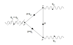
Figure 1: The axial-vector-vector 3-point function. Wavy lines correspond to vector currents and wavy slashed line corresponds to the axial vector current.

The probability amplitude for the axial-vector-vector process is represented by the triangle diagram, depicted on fig. 1. In order to compute it in the SQM, one needs to find a spectral representation to the vertex function with one axial and one vector current, $\Lambda^{\mu a;\nu b}_{AV}$, that fulfills the $SU(2)$ vector and axial vector Ward identities.

For non-local axial vertex in the chiral limit, the axial Ward identity reads:

$$-iq_{\mu}\Lambda^{\mu a;\nu b}_{AV}(p^{\prime},q^{\prime},p,q)=i\epsilon_{bac}\Lambda^{\nu c}_{A}(p^{\prime},p)\Big{|}_{g_{A}=1}$$

$$+\Lambda^{\nu b}_{V}(p^{\prime},p+q)\gamma^{5}\frac{\tau_{a}}{2}+\gamma^{5}\frac{\tau_{a}}{2}\Lambda^{\nu b}_{V}(p^{\prime}-q,p),$$ (26)

The first term on the right hand side of Eq.(26) is the axial vertex computed with $g_{A}=1$. This term express the fact that the contraction of the axial vertex with the exchanged momentum does not depends on $g_{A}$, as can be easily checked by evaluating $q_{\mu}\Lambda^{\mu a}_{A}$ from Eq. (21) with the use of Eqs.(22) and (23).

The vector Ward identity reads:

$$-iq^{\prime}_{\nu}\Lambda^{\mu a;\nu b}_{AV}(p^{\prime},q^{\prime},p,q)=i\epsilon_{bac}\Lambda^{\mu c}_{A}(p^{\prime},p)$$

$$-\Lambda^{\mu b}_{A}(p+q,p)\frac{\tau_{a}}{2}-\frac{\tau_{a}}{2}\Lambda^{\mu b}_{A}(p^{\prime},p^{\prime}-q).$$ (27)

A solution that fulfills Eq.(27) and Eq.(26) in the chiral limit is given by:

$$\Lambda^{\mu a;\nu b}_{AV}(p^{\prime},q^{\prime},p,q)=\int d\omega\rho(\omega)\Big{\{}\frac{i}{\hbox to0.0pt{\hbox to5.03125pt{\hfil/\hfil}\hss}p^{\prime}-\omega}\gamma^{\nu}\frac{\tau^{b}}{2}\frac{i}{\hbox to0.0pt{\hbox to5.03125pt{\hfil/\hfil}\hss}p+\hbox to0.0pt{\hbox to5.00002pt{\hfil$q$\hfil}\hss}/-\omega}$$

$$\times\Big{(}g_{A}\gamma^{\mu}-2\omega\frac{q^{\mu}}{q^{2}}+(1-g_{A})\frac{q^{\mu}\hbox to0.0pt{\hbox to5.00002pt{\hfil$q$\hfil}\hss}/}{q^{2}}\Big{)}\gamma^{5}\frac{\tau_{a}}{2}\frac{i}{\hbox to0.0pt{\hbox to5.03125pt{\hfil/\hfil}\hss}p-\omega}$$

$$+\frac{i}{\hbox to0.0pt{\hbox to5.03125pt{\hfil/\hfil}\hss}p^{\prime}-\omega}\Big{(}g_{A}\gamma^{\mu}-2\omega\frac{q^{\mu}}{q^{2}}+(1-g_{A})\frac{q^{\mu}\hbox to0.0pt{\hbox to5.00002pt{\hfil$q$\hfil}\hss}/}{q^{2}}\Big{)}\gamma^{5}\frac{\tau_{a}}{2}$$

$$\times\frac{i}{\hbox to0.0pt{\hbox to5.03125pt{\hfil/\hfil}\hss}p^{\prime}-\hbox to0.0pt{\hbox to5.00002pt{\hfil$q$\hfil}\hss}/-\omega}\gamma^{\nu}\frac{\tau^{b}}{2}\frac{i}{\hbox to0.0pt{\hbox to5.03125pt{\hfil/\hfil}\hss}p-\omega}\Big{\}},$$ (28)

with $p^{\prime}+q^{\prime}=p+q$. In fact, replacing Eq.(28) in Eq.(26) one obtains:

$$-iq_{\mu}\Lambda^{\mu a;\nu b}_{AV}(p^{\prime},q^{\prime},p,q)=i\epsilon_{bac}\Lambda^{\nu c}_{A}(p^{\prime},p)\Big{|}_{g_{A}=1}$$

$$+\Lambda^{\nu b}_{V}(p^{\prime},p+q)\gamma^{5}\frac{\tau_{a}}{2}+\gamma^{5}\frac{\tau_{a}}{2}\Lambda^{\nu b}_{V}(p^{\prime}-q,p)$$

$$+i2\epsilon_{bac}\frac{q^{\nu}}{q^{2}}\int d\omega\rho(\omega)\omega\frac{i}{\hbox to0.0pt{\hbox to5.03125pt{\hfil/\hfil}\hss}p^{\prime}-\omega}\gamma^{5}\frac{\tau^{c}}{2}\frac{i}{\hbox to0.0pt{\hbox to5.03125pt{\hfil/\hfil}\hss}p-\omega}$$ (29)

Eq.(29) displays the expected partial conservation of the axial current. This can be verified by evaluating the last term in Eq.(29) with $\hbox to0.0pt{\hbox to5.03125pt{\hfil/\hfil}\hss}p^{\prime}=\hbox to0.0pt{\hbox to5.03125pt{\hfil/\hfil}\hss}p$, resulting in

$$\Big{\{}2i\epsilon_{bac}\frac{q^{\nu}}{q^{2}}\int d\omega\rho(\omega)\omega\frac{i}{\hbox to0.0pt{\hbox to5.03125pt{\hfil/\hfil}\hss}p^{\prime}-\omega}\gamma^{5}\frac{\tau^{c}}{2}\frac{i}{\hbox to0.0pt{\hbox to5.03125pt{\hfil/\hfil}\hss}p-\omega}\Big{\}}_{\hbox to0.0pt{\hbox to3.52188pt{\hfil/\hfil}\hss}p^{\prime}=\hbox to0.0pt{\hbox to3.52188pt{\hfil/\hfil}\hss}p}$$

$$=\Big{\{}2i\epsilon_{bac}\frac{q^{\nu}}{q^{2}}\int d\omega\rho(\omega)\omega\frac{\hbox to0.0pt{\hbox to5.03125pt{\hfil/\hfil}\hss}p^{\prime}\hbox to0.0pt{\hbox to5.03125pt{\hfil/\hfil}\hss}p-\omega^{2}-\omega(\hbox to0.0pt{\hbox to5.03125pt{\hfil/\hfil}\hss}p^{\prime}-\hbox to0.0pt{\hbox to5.03125pt{\hfil/\hfil}\hss}p)}{(p^{\prime 2}-\omega^{2})(p^{2}-\omega^{2})}\gamma^{5}\frac{\tau^{c}}{2}\Big{\}}_{\hbox to0.0pt{\hbox to3.52188pt{\hfil/\hfil}\hss}p^{\prime}=\hbox to0.0pt{\hbox to3.52188pt{\hfil/\hfil}\hss}p}$$

$$=2i\epsilon_{bac}\frac{q^{\nu}}{q^{2}}\gamma^{5}\frac{\tau^{c}}{2}\int d\omega\rho(\omega)\frac{\omega}{(p^{2}-\omega^{2})}$$

$$=2i\epsilon_{bac}m(p)\frac{q^{\nu}}{q^{2}}\gamma^{5}\frac{\tau^{c}}{2}\int d\omega\rho(\omega)\frac{1}{(p^{2}-\omega^{2})}$$ (30)

where we have made use of Eq.(9). So, the last term of Eq.(29) shows the violation of the axial current conservation arising from the fermionic mass term, as usual. When chiral symmetry is restored, Eq.(30) will vanish, and the axial Ward identity, Eq.(26), will be fulfilled by the solution (28).

In the SQM the probability amplitude for the axial-vector-vector process is obtained by closing the quark line in the unamputated two currents (axial and vector) vertex, Eq.(28). With the appropriated insertion of the charge matrices, and the momenta labels chosen as in Fig.(1), this probability amplitude is given by:

$$T^{AVV}_{\rho\mu\nu}(q_{1},q_{2})=-\int d\omega\rho(\omega)\int_{p}Tr\bigg{[}N_{C}i\tau^{3}$$

$$\Big{(}g_{A}(\omega)\gamma_{\rho}-\frac{2\omega}{q^{2}}q_{\rho}+\frac{1-g_{A}(\omega)}{q^{2}}q_{\rho}{\hbox to0.0pt{\hbox to5.00002pt{\hfil$q$\hfil}\hss}/}\Big{)}\gamma_{5}\frac{i}{{\hbox to0.0pt{\hbox to5.03125pt{\hfil/\hfil}\hss}p}+{\hbox to0.0pt{\hbox to5.00002pt{\hfil$q$\hfil}\hss}/}_{1}-\omega}$$

$$i\hat{Q}\gamma_{\mu}\frac{i}{{\hbox to0.0pt{\hbox to5.03125pt{\hfil/\hfil}\hss}p}-\omega}i\hat{Q}\gamma_{\nu}\frac{i}{{\hbox to0.0pt{\hbox to5.03125pt{\hfil/\hfil}\hss}p}-{\hbox to0.0pt{\hbox to5.00002pt{\hfil$q$\hfil}\hss}/}_{2}-\omega}\bigg{]}+\text{crossed terms},$$ (31)

where $\hat{Q}$ is the quark charge matrix, $q=q_{1}+q_{2}$ and, for a $SU(2)$ model, $\tau^{3}$ is the Pauli matrix $\sigma_{z}$. In order to compare with the PCAC relation, let us rewrite the term proportional to $\frac{\omega}{q^{2}}q_{\rho}$ as

$$T_{\mu\nu}=\frac{1}{m}\int d\omega\rho(\omega)\omega\int_{p}Tr\bigg{\{}\frac{\gamma_{5}({\hbox to0.0pt{\hbox to5.03125pt{\hfil/\hfil}\hss}p}+{\hbox to0.0pt{\hbox to5.00002pt{\hfil$q$\hfil}\hss}/}_{1}+\omega)}{((p+q_{1})^{2}-\omega^{2})}\times$$

$$\frac{\gamma_{\mu}({\hbox to0.0pt{\hbox to5.03125pt{\hfil/\hfil}\hss}p}+\omega)\gamma_{\nu}({\hbox to0.0pt{\hbox to5.03125pt{\hfil/\hfil}\hss}p}-{\hbox to0.0pt{\hbox to5.00002pt{\hfil$q$\hfil}\hss}/}_{2}+\omega)}{(p^{2}-\omega^{2})((p-q_{2})^{2}-\omega^{2})}\bigg{\}}+\text{crossed terms}$$ (32)

where we have introduced the mass function at zero external momentum $m$ in order to associate $T_{\mu\nu}$ with the standard representation of the neutral pion to two photons decay amplitude. Eq.(31), of course, does not depend on $m$, and can be rewritten as

$$T^{AVV}_{\rho\mu\nu}(q_{1},q_{2})=\lambda\Big{(}\hat{T}_{\rho\mu\nu}+\frac{q_{\rho}}{q^{2}}2mT_{\mu\nu}+\frac{q_{\rho}}{q^{2}}T^{*}_{\mu\nu}\Big{)},$$ (33)

with

$$\hat{T}_{\rho\mu\nu}=\int d\omega\rho(\omega)g_{A}(\omega)\int_{p}Tr\bigg{\{}\frac{\gamma_{\rho}\gamma_{5}({\hbox to0.0pt{\hbox to5.03125pt{\hfil/\hfil}\hss}p}+{\hbox to0.0pt{\hbox to5.00002pt{\hfil$q$\hfil}\hss}/}_{1}+\omega)}{((p+q_{1})^{2}-\omega^{2})}\times$$

$$\frac{\gamma_{\mu}({\hbox to0.0pt{\hbox to5.03125pt{\hfil/\hfil}\hss}p}+\omega)\gamma_{\nu}({\hbox to0.0pt{\hbox to5.03125pt{\hfil/\hfil}\hss}p}-{\hbox to0.0pt{\hbox to5.00002pt{\hfil$q$\hfil}\hss}/}_{2}+\omega)}{(p^{2}-\omega^{2})((p-q_{2})^{2}-\omega^{2})}\bigg{\}}+\text{crossed terms}$$ (34)

and

$$T^{*}_{\mu\nu}=\int d\omega\rho(\omega)(1-g_{A}(\omega))\int_{p}Tr\bigg{\{}\frac{{\hbox to0.0pt{\hbox to5.00002pt{\hfil$q$\hfil}\hss}/}\gamma_{5}({\hbox to0.0pt{\hbox to5.03125pt{\hfil/\hfil}\hss}p}+{\hbox to0.0pt{\hbox to5.00002pt{\hfil$q$\hfil}\hss}/}_{1}+\omega)}{((p+q_{1})^{2}-\omega^{2})}\times$$

$$\frac{\gamma_{\mu}({\hbox to0.0pt{\hbox to5.03125pt{\hfil/\hfil}\hss}p}+\omega)\gamma_{\nu}({\hbox to0.0pt{\hbox to5.03125pt{\hfil/\hfil}\hss}p}-{\hbox to0.0pt{\hbox to5.00002pt{\hfil$q$\hfil}\hss}/}_{2}+\omega)}{(p^{2}-\omega^{2})((p-q_{2})^{2}-\omega^{2})}\bigg{\}}+\text{crossed terms}.$$ (35)

We also have

$$\lambda=N_{c}Tr\{\tau^{3}\hat{Q}\hat{Q}\}=1.$$ (36)

It is interesting to note that, after taking the Dirac traces, Eq.(32) is logarithmically divergent, and thus does not present surface terms in its computation. Eq.(35) is quadratically divergent, and in principle should present surface terms. However, in the sharp cutoff regularization scheme these surface terms result zero. After a little algebra, we obtain

$$T^{*}_{\mu\nu}=\frac{1}{2\pi^{2}}\epsilon_{\rho\mu\nu\eta}q_{1}^{\rho}q_{2}^{\eta}\int d\omega\rho(\omega)(1-g_{A}(\omega)),$$ (37)

and

$$2mT_{\mu\nu}=\frac{2}{4\pi^{2}}\epsilon_{\mu\nu\rho\eta}q_{1}^{\eta}q_{2}^{\rho}\int d\omega\rho(\omega).$$ (38)

Eq.(34), however, presents non-null surface terms in its calculation. These surface terms come from the difference of logarithmically divergent integrals, the same integrals in $p$ appearing in Eq.(20),

$$\int_{p}\Big{(}\frac{g^{\mu\nu}}{(p^{2}-\omega^{2})^{2}}-4\frac{p^{\mu}p^{\nu}}{(p^{2}-\omega^{2})^{3}}\Big{)}.$$ (39)

As already discussed, this term corresponds to a regularization ambiguity, since it can result zero in some regularizations (e.g. gauge invariant Pauli-Villars) or finite in other ones ($=\frac{i}{2(4\pi^{2})}$ in the sharp cutoff regularization) . So, introducing two Feynman parameters on Eq.(34) we obtain

$$\hat{T}_{\rho\mu\nu}=\int d\omega\rho(\omega)g_{A}(\omega)\int_{0}^{1}dy\int_{0}^{1-y}dx$$ (40)

$$\times\int_{p}\frac{Tr\{\gamma_{\rho}\gamma_{5}(\hbox to0.0pt{\hbox to5.03125pt{\hfil/\hfil}\hss}p+\hbox to0.0pt{\hbox to5.00002pt{\hfil$q$\hfil}\hss}/_{1}+\omega)\gamma_{\mu}(\hbox to0.0pt{\hbox to5.03125pt{\hfil/\hfil}\hss}p+\omega)\gamma_{\nu}(\hbox to0.0pt{\hbox to5.03125pt{\hfil/\hfil}\hss}p-\hbox to0.0pt{\hbox to5.00002pt{\hfil$q$\hfil}\hss}/_{2}+\omega)\}}{((p+q_{1}x-q_{2}y)^{2}-M^{2}(\omega,x,y))^{3}},$$

with $M^{2}(\omega,x,y)=q_{1}^{2}x(x-1)+q_{2}^{2}y(y-1)-2q_{1}q_{2}xy+\omega^{2}$ (the sharp cut-off regularization scheme is, as before, implicitly assumed). In several regularization schemes, as in the sharp-cutoff, we are not allowed to shift the $p$ variable in Eq.(40), unless we introduce the corresponding surface term. Following the procedure employed in Ref. Battistel et al. (1998), we obtain

$$\hat{T}_{\rho\mu\nu}=S_{\rho\mu\nu}+\int d\omega\rho(\omega)g_{A}(\omega)\int_{0}^{1}dy\int_{0}^{1-y}dx$$

$$\times\int_{p}\frac{1}{(p^{2}-M^{2}(\omega,x,y))^{3}}$$

$$\times Tr\{\gamma_{\rho}\gamma_{5}(\hbox to0.0pt{\hbox to5.03125pt{\hfil/\hfil}\hss}p+(1-x)\hbox to0.0pt{\hbox to5.00002pt{\hfil$q$\hfil}\hss}/_{1}+y\hbox to0.0pt{\hbox to5.00002pt{\hfil$q$\hfil}\hss}/_{2}+\omega)\gamma_{\mu}(\hbox to0.0pt{\hbox to5.03125pt{\hfil/\hfil}\hss}p-x\hbox to0.0pt{\hbox to5.00002pt{\hfil$q$\hfil}\hss}/_{1}$$

$$+y\hbox to0.0pt{\hbox to5.00002pt{\hfil$q$\hfil}\hss}/_{2}+\omega)\gamma_{\nu}(\hbox to0.0pt{\hbox to5.03125pt{\hfil/\hfil}\hss}p-x\hbox to0.0pt{\hbox to5.00002pt{\hfil$q$\hfil}\hss}/_{1}-(1-y)\hbox to0.0pt{\hbox to5.00002pt{\hfil$q$\hfil}\hss}/_{2}+\omega)\},$$ (41)

where $S_{\rho\mu\nu}$ is the surface term given by

$$S_{\rho\mu\nu}=\int d\omega\rho(\omega)g_{A}(\omega)\int_{0}^{1}dy\int_{0}^{1-y}dx$$

$$\times\int_{p}(q_{1}^{\sigma}x-q_{2}^{\sigma}y)\frac{\partial}{\partial p^{\sigma}}\Big{\{}\frac{Tr\{\gamma_{\rho}\gamma_{5}\hbox to0.0pt{\hbox to5.03125pt{\hfil/\hfil}\hss}p\gamma_{\mu}\hbox to0.0pt{\hbox to5.03125pt{\hfil/\hfil}\hss}p\gamma_{\nu}\hbox to0.0pt{\hbox to5.03125pt{\hfil/\hfil}\hss}p\}}{(p^{2}-M^{2}(\omega,x,y))^{3}}\Big{\}}$$ (42)

Of course, as usual, $T^{AVV}_{\rho\mu\nu}$ is finite, so all integrals can be computed and the connection limit $\Lambda\rightarrow\infty$ can be taken. After doing that, we have

$$\hat{T}_{\rho\mu\nu}=\frac{1}{4\pi^{2}}\bigg{\{}\int d\omega\frac{g_{A}(\omega)\rho(\omega)}{6\omega^{2}}q_{1}^{\eta}q_{2}^{\beta}\{\epsilon_{\rho\mu\beta\eta}(q_{2\nu}+2q_{1\nu})$$

$$+\epsilon_{\rho\beta\nu\eta}(2q_{2\mu}+q_{1\mu})\}$$

$$+\frac{2}{3}\epsilon_{\rho\mu\nu\eta}\int d\omega\rho(\omega)g_{A}(\omega)(q_{2}^{\eta}-q_{1}^{\eta})\bigg{\}}+S_{\rho\mu\nu}$$ (43)

with

$$S_{\rho\mu\nu}=\frac{1}{12\pi^{2}}\epsilon_{\rho\mu\nu\eta}\int d\omega\rho(\omega)g_{A}(\omega)(q_{2}^{\eta}-q_{1}^{\eta})$$ (44)

From Eqs. (33), (43) and (37), the evaluation of the Ward-Takahashi identities in momentum space results in

$$q_{1}^{\mu}T^{AVV}_{\rho\mu\nu}=\frac{1}{4\pi^{2}}\frac{2}{3}q_{1}^{\mu}q_{2}^{\eta}\epsilon_{\mu\nu\rho\eta}\int d\omega\rho(\omega)g_{A}(\omega)$$

$$+q_{1}^{\mu}S_{\rho\mu\nu},$$ (45)

for the VWI, with a similar expression for $q_{2}^{\nu}T^{AVV}_{\rho\mu\nu}$, and

$$(q_{1}^{\rho}+q_{2}^{\rho})T^{AVV}_{\rho\mu\nu}=\frac{2}{4\pi^{2}}q_{1}^{\eta}q_{2}^{\rho}\epsilon_{\mu\nu\rho\eta}\frac{1}{3}\int d\omega\rho(\omega)g_{A}(\omega)$$

$$+(q_{1}^{\rho}+q_{2}^{\rho})S_{\rho\mu\nu}+2mT_{\mu\nu}-\frac{2}{4\pi^{2}}q_{1}^{\eta}q_{2}^{\rho}\epsilon_{\mu\nu\rho\eta},$$ (46)

for the AWI.

Before performing the spectral mass integrals, the result is potentially ambiguous due the presence of the surface term $S_{\rho\mu\nu}$ in Eqs.(43), (45) and (46). For a constant ($\omega$ independent) $g_{A}$, the surface term, Eq.(44), depends on the choice of the intermediary regularization employed in the evaluation of Eq.(31), and it could generate different results in the Ward identity to be violated by the anomaly, as it is well known.

Nevertheless, from Eq.(44) we can see that the computation of the axial-vector-vector amplitude in the SQM with the axial vertex given by Eq.(21) and with $g_{A}=\alpha\omega$ (or $g_{A}=\alpha\omega^{2}$) is free from surface terms - the spectral condition, Eq.(3), ensures their vanishing, as well as the vanishing of the other terms proportional to $g_{A}(\omega)$ in Eqs.(45) and (46). In this case, the VWI is always preserved (i.e., is preserved in an ambiguity free way) and the AWI is violated. Hence, we clearly see that the choice of the specific dependence of the axial coupling with the spectral mass can result in an ambiguity free result, with the conservation of the VWI, and the violation of the chiral one, as expected for QCD. In this case, the vanishing of the spectral axial coupling in the zero spectral mass limit does not imply in the vanishing of the axial coupling itself. However, it is also possible to obtain the violation of the VWI, with conservation of the axial current, when the spectral axial coupling depends on the spectral mass with a power lower than 1. In this case, the presence of ambiguous terms implies in the freedom on choosing which Ward identity is to be violated.

VI Conclusions

We have investigated the chiral anomaly in the context of the Spectral Quark Model. We have proposed a generalized form of the four points vertex function with one axial and one vector current which includes the possibility of a non unitary, spectral mass dependent, axial coupling. This vertex function displays the expected partial conservation of the axial current, with the chiral Ward identity being violated by a term proportional to the mass function which vanishes at the chiral limit. The triangle anomaly was computed, taking into account the surface term that appears in its calculation, and we have shown that a dependence of the axial coupling on integer positive powers of the spectral mass is necessary in order to render the triangle amplitude free from ambiguities. In this case, the vector Ward identity is preserved, with the chiral Ward identity being violated as expected for QCD. We also remarked that the dependence of the pion to quarks couplings on the spectral mass, via the Goldberger-Treiman relation for the pseudoscalar coupling, and via the ansatz employed here for the axial coupling, are essential to the obtaining of a result free from divergences and regularization ambiguities.

In summary, we have shown that, in the context of the Spectral Quark Model, the chiral anomaly computation can be carried out reproducing the expected result without any ambiguity introduced by regularizations schemes, if the axial vertex is treated as a non-local spectral mass dependent vertex. This shows to be compatible with an non-unitary axial vector coupling, not vanishing at the chiral limit. Our result suggests that the Spectral Quark Model provides an useful mechanism to justify why in QCD the anomaly violates the chiral symmetry, instead of violating gauge symmetry, as in the case of the non conservation of the barionic number. However, we also discussed that the more general form for the axial vertex leaves room to the violation of the vector Ward Identity, complying the axial one. It could be interesting to analyze these features of the Spectral Quark Model in the QCD chiral phase transition Chandrasekharan and Mehta (2006, 2007) or in the construction of spectral approaches to some recent applications of the chiral anomaly Bracken (2008); Benfatto and Mastropietro (2005); Sasaki (2002); Klebanov et al. (2002).

VII Acknowledgments

This research was supported by CAPES-Brazil. The authors would like to thank H. Caldas for carefully reading the manuscript.

References

- Gell-Mann and L’evy (1960) M. Gell-Mann and M. L’evy, Nuovo Cim. 16, 705 (1960).
- Nambu and Jona-Lasinio (1961a) Y. Nambu and G. Jona-Lasinio, Phys. Rev. 124, 246 (1961a).
- Nambu and Jona-Lasinio (1961b) Y. Nambu and G. Jona-Lasinio, Phys. Rev. 122, 345 (1961b).
- Ram Mohan (1976) L. R. Ram Mohan, Phys. Rev. D14, 2670 (1976).
- Asakawa and Yazaki (1989) M. Asakawa and K. Yazaki, Nucl. Phys. A504, 668 (1989).
- Klimt et al. (1990) S. Klimt, M. Lutz, and W. Weise, Phys. Lett. B249, 386 (1990).
- Kunihiro (1991) T. Kunihiro, Nucl. Phys. B351, 593 (1991).
- Caldas (2004) H. Caldas, Phys. Rev. C69, 035204 (2004), eprint hep-ph/0308058.
- Caldas and Nemes (2001) H. C. G. Caldas and M. C. Nemes, Phys. Lett. B523, 293 (2001), eprint hep-th/0107249.
- Caldas et al. (2001) H. C. G. Caldas, A. L. Mota, and M. C. Nemes, Phys. Rev. D63, 056011 (2001), eprint hep-ph/0005180.
- Caldas et al. (1997) H. C. G. Caldas, D. H. T. Franco, A. L. Mota, F. A. Oliveira, and M. C. Nemes, Nucl. Phys. A617, 464 (1997).
- Andersen et al. (2004) J. O. Andersen, D. Boer, and H. J. Warringa, Phys. Rev. D70, 116007 (2004), eprint hep-ph/0408033.
- Andersen and Brauner (2008) J. O. Andersen and T. Brauner, Phys. Rev. D78, 014030 (2008), eprint 0804.4604.
- Petropoulos (1999) N. Petropoulos, J. Phys. G25, 2225 (1999), eprint hep-ph/9807331.
- Roh and Matsui (1998) H.-S. Roh and T. Matsui, Eur. Phys. J. A1, 205 (1998), eprint nucl-th/9611050.
- Goldberg (1983) H. Goldberg, Phys. Lett. B131, 133 (1983).
- Lenaghan et al. (2000) J. T. Lenaghan, D. H. Rischke, and J. Schaffner-Bielich, Phys. Rev. D62, 085008 (2000), eprint nucl-th/0004006.
- Baym and Grinstein (1977) G. Baym and G. Grinstein, Phys. Rev. D15, 2897 (1977).
- Reinhardt and Dang (1987) H. Reinhardt and B. V. Dang, J. Phys. G13, 1179 (1987).
- Christov et al. (1991) C. V. Christov, E. Ruiz Arriola, and K. Goeke, Acta Phys. Polon. B22, 187 (1991).
- Ebert et al. (1993) D. Ebert, Y. L. Kalinovsky, L. Munchow, and M. K. Volkov, Int. J. Mod. Phys. A8, 1295 (1993).
- Schwarz et al. (1999) T. M. Schwarz, S. P. Klevansky, and G. Papp, Phys. Rev. C60, 055205 (1999), eprint nucl-th/9903048.
- Blin et al. (1988) A. H. Blin, B. Hiller, and M. Schaden, Z. Phys. A331, 75 (1988).
- Ruiz Arriola (2002) E. Ruiz Arriola, Acta Phys. Polon. B33, 4443 (2002), eprint hep-ph/0210007.
- Battistel et al. (1998) O. A. Battistel, A. L. Mota, and M. C. Nemes, Mod. Phys. Lett. A13, 1597 (1998).
- Baeta Scarpelli et al. (2001) A. P. Baeta Scarpelli, M. Sampaio, B. Hiller, and M. C. Nemes, Phys. Rev. D64, 046013 (2001), eprint hep-th/0102108.
- Freedman et al. (1992) D. Z. Freedman, K. Johnson, and J. I. Latorre, Nucl. Phys. B371, 353 (1992).
- Jackiw (2000a) R. Jackiw, Int. J. Mod. Phys. B14, 2011 (2000a), eprint hep-th/9903044.
- ’t Hooft (1976) G. ’t Hooft, Phys. Rev. Lett. 37, 8 (1976).
- Jackiw (2000b) R. Jackiw (2000b), eprint hep-th/0011274.
- Jackiw and Kostelecky (1999) R. Jackiw and V. A. Kostelecky, Phys. Rev. Lett. 82, 3572 (1999), eprint hep-ph/9901358.
- Perez-Victoria (1999) M. Perez-Victoria, Phys. Rev. Lett. 83, 2518 (1999), eprint hep-th/9905061.
- Chung (1999) J. M. Chung, Phys. Lett. B461, 138 (1999), eprint hep-th/9905095.
- Andrianov et al. (2002) A. A. Andrianov, P. Giacconi, and R. Soldati, JHEP 02, 030 (2002), eprint hep-th/0110279.
- Bonneau (2001) G. Bonneau, Nucl. Phys. B593, 398 (2001), eprint hep-th/0008210.
- Bonneau (2007) G. Bonneau, Nucl. Phys. B764, 83 (2007), eprint hep-th/0611009.
- Ruiz Arriola and Broniowski (2003a) E. Ruiz Arriola and W. Broniowski, Phys. Rev. D67, 074021 (2003a), eprint hep-ph/0301202.
- Ruiz Arriola and Broniowski (2003b) E. Ruiz Arriola and W. Broniowski (2003b), eprint hep-ph/0310044.
- Megias et al. (2004) E. Megias, E. Ruiz Arriola, L. L. Salcedo, and W. Broniowski, Phys. Rev. D70, 034031 (2004), eprint hep-ph/0403139.
- Arriola et al. (2007) E. R. Arriola, W. Broniowski, and B. Golli, Phys. Rev. D76, 014008 (2007), eprint hep-ph/0610289.
- Broniowski and Arriola (2007) W. Broniowski and E. R. Arriola, Phys. Lett. B649, 49 (2007), eprint hep-ph/0701243.
- Itzykson and Zuber (1980) C. Itzykson and J. B. Zuber (1980), new York, Usa: Mcgraw-hill (1980) 705 P.(International Series In Pure and Applied Physics).
- Delbourgo and West (1977) R. Delbourgo and P. C. West, J. Phys. A10, 1049 (1977).
- Delbourgo (1979) R. Delbourgo, Nuovo Cim. A49, 484 (1979).
- Goldberger and Treiman (1958) M. L. Goldberger and S. B. Treiman, Phys. Rev. 110, 1178 (1958).
- Broniowski et al. (1993) W. Broniowski, A. Steiner, and M. Lutz, Phys. Rev. Lett. 71, 1787 (1993), eprint hep-ph/9304292.
- Carter (2003) G. W. Carter, Phys. Rev. D67, 014008 (2003), eprint hep-ph/0208250.
- Groom et al. (2000) D. E. Groom et al. (Particle Data Group), Eur. Phys. J. C15, 1 (2000).
- Volmer et al. (2001) J. Volmer et al. (The Jefferson Lab F(pi)), Phys. Rev. Lett. 86, 1713 (2001), eprint nucl-ex/0010009.
- Klevansky (1992) S. P. Klevansky, Rev. Mod. Phys. 64, 649 (1992).
- Dias et al. (2006) E. W. Dias et al., Mod. Phys. Lett. A21, 339 (2006), eprint hep-ph/0503245.
- Hiller et al. (2006) B. Hiller, A. L. Mota, M. C. Nemes, A. A. Osipov, and M. Sampaio, Nucl. Phys. A769, 53 (2006), eprint hep-ph/0503205.
- Bell and Jackiw (1969) J. S. Bell and R. Jackiw, Nuovo Cim. A60, 47 (1969).
- Adler (1969) S. L. Adler, Phys. Rev. 177, 2426 (1969).
- Chandrasekharan and Mehta (2006) S. Chandrasekharan and A. C. Mehta, PoS LAT2006, 128 (2006), eprint hep-lat/0611025.
- Chandrasekharan and Mehta (2007) S. Chandrasekharan and A. C. Mehta, Phys. Rev. Lett. 99, 142004 (2007), eprint 0705.0617.
- Bracken (2008) P. Bracken, Int. J. Mod. Phys. B22, 2675 (2008).
- Benfatto and Mastropietro (2005) G. Benfatto and V. Mastropietro, Commun. Math. Phys. 258, 609 (2005), eprint cond-mat/0409049.
- Sasaki (2002) K. Sasaki, Phys. Lett. A296, 237 (2002), eprint cond-mat/0104556.
- Klebanov et al. (2002) I. R. Klebanov, P. Ouyang, and E. Witten, Phys. Rev. D65, 105007 (2002), eprint hep-th/0202056.