String coupling and interactions in type IIB matrix model

Abstract

We investigate the interactions of closed strings in IIB matrix model. The basic interaction of the closed superstring is realized by the recombination of two intersecting strings. Such interaction is investigated in IIB matrix model via two dimensional noncommutative gauge theory in the IR limit. By estimating the probability of the recombination, we identify the string coupling $g_{s}$ in IIB matrix model. We confirm that our identification is consistent with matrix string theory.

I Introduction

IIB matrix model IKKT is considered as a candidate of the nonperturbative formulation of superstring theory. The relation between IIB matrix model and perturbative string theory is shown in KN3 . Perturbative string theory is also contained in Dijkgraaf, Verlinde and Verlinde’s matrix string theory DVV . Strong coupling region of two dimensional supersymmetric Yang-Mills theory is described by the perturbative superstring theory. In the strong coupling limit, a free Green-Schwarz string theory is obtained. On the other hand, weak coupling region is described by the perturbative Yang-Mills theory. In addition, there is an intermediate region which is described by type IIB supergravity solution in the large $N$ limit IMSY .

The aim of this paper is to identify the string coupling $g_{s}$ in IIB matrix model. The hint for the identification comes from the matrix string theory. The gauge coupling of the two dimensional Yang-Mills theory has the $[length]^{-1}$ of the worldsheet and it is related to the string coupling as $g_{YM}^{-2}=\alpha^{\prime}g_{s}^{2}$. The $g_{s}$ has the dimension $[length]$ on the worldsheet. Thus, our task is to search for the dimensionful parameter on the worldsheet.

Before searching for $g_{s}$, we have to construct the worldsheets in IIB matrix model. They are constructed as two dimensional classical backgrounds KN3 in the IR limit. The string length is identified there and free multiple closed strings are obtained. Vertex operators of type IIA superstring are constructed from IIB matrix model on these backgrounds in KN4 . The relation between type IIA superstring theory and IIB matrix model is also proposed in KS in a different way.

In this paper, we consider the interaction of perturbative strings. The basic interactions are the transitions from two strings into one string or vice versa. These interactions are introduced in the formulation of superstring field theory in the light-cone gauge GSB . 2 strings $\to$ 1 string interactions are represented by the recombination of intersecting strings locally. See figure 1.

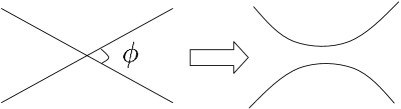
Figure 1: Two strings intersect at an angle $\phi$. The recombination happens at the intersection point.

Although this process locally represents the recombination of 2 strings $\to$ 2 strings, the final state is connected globally. Thus, after the recombination, we obtain a single closed string. In the matrix model, the instability of this system comes from the off-diagonal modes. The system with the larger intersection angle $\phi$ is more unstable than that with the smaller intersection angle. In other words, the decay rate of two closed strings is decided by the intersection angle $\phi$. We can replace the angle $\phi$ with another parameter $q$ which is related to $\phi$ as $\phi=2\tan^{-1}q$. Since we choose the horizontal axis in figure 1 as the coordinate of the worldsheet $\sigma$ and the vertical axis as the transverse scalar field $\phi_{i}(\sigma)$, the parameter $q$ denotes the slope of the tilted strings. In the two dimensional gauge theory, $q$ is the dimensionful parameter. We clarify the $q$ dependence of the instability. Since the configuration decays into the single closed string through the recombination process, we estimate $q$ dependence of the recombination probability. In the string perturbation theory, the recombination probability is proportional to $g_{s}^{2}$ to the leading order.

In our investigation, we derive the action of multiple strings from IIB matrix model. We identify the unstable mode for the intersecting strings which are the solutions of this action. From this mode, we estimate the probability of the recombination. By comparing the result to that of the perturbative string theory, we identify the string coupling $g_{s}$ in IIB matrix model.

In section 2, we derive the action of multiple closed superstrings. In section 3.1, we carry out the fluctuation analysis for the intersecting closed strings. We identify the unstable mode. In section 3.2, we calculate the probability of the recombination from the unstable mode. By comparing our result with that of the perturbative superstring theory, we identify the string coupling $g_{s}$. In section 3.3, we estimate the probability of the recombination in matrix string theory. Section 4 is devoted to the conclusion. In the appendix A, our notation of light-cone coordinates is given. In the appendix B.1, the differential equations for the fluctuation modes are solved. In the appendix B.2, the Schrodinger equation which controls the time evolution of the probability is solved.

II The effective action of multiple strings

The interaction among multiple strings is described in various ways in string theory. Perturbatively, transitions from two strings into one string or vice versa are the basic process. We aim to identify such interactions in IIB matrix model. Since this interaction is proportional to $g_{s}$ at the tree level, we can identify $g_{s}$ in IIB matrix model through this process.

Let us start from the action

$$S=-\frac{1}{g^{2}}{\rm Tr}\left(\frac{1}{4}[A^{\mu},A^{\nu}][A_{\mu},A_{\nu}]+\frac{1}{2}\bar{\psi}\Gamma^{\mu}[A_{\mu},\psi]\right)\ ,\hskip 8.5359pt$$ (II.1)

where $\psi$ is a ten dimensional Majorana-Weyl spinor and $A_{\mu}(\mu=0,1,\cdots,9)$ and $\psi$ are $N\times N$ Hermitian matrices. By expanding the action (II.1) around a two dimensional noncommutative background,

$$[p_{\mu},p_{\nu}]=i\theta_{\mu\nu}\ ,$$ (II.2)

we obtain an ${\cal N}=8$ two dimensional $U(n)$ noncommutative gauge theory CDS ; AIIKKT ; Li

$$S=-\frac{\theta}{8\pi g^{2}}\int d^{2}x{\rm tr}\left(F^{2}_{\tilde{\mu}\tilde{\nu}}+2(D_{\tilde{\mu}}\phi_{i})^{2}+[\phi_{i},\phi_{j}][\phi_{i},\phi_{j}]\right.$$

$$\left.+2\bar{\psi}\Gamma^{\tilde{\mu}}D_{\tilde{\mu}}\psi+2\bar{\psi}\Gamma_{i}[\phi_{i},\psi]\right)_{*}\ ,\hskip 28.45274pt$$ (II.3)

where $\tilde{\mu},\tilde{\nu}=0,1$ and $i,j=2,\cdots,9$.

The $*$ product is described by

$$a*b=\exp\left(\frac{iC^{\mu\nu}}{2}\frac{\partial^{2}}{\partial\xi^{\mu}\partial\eta^{\nu}}\right)a(x+\xi)b(x+\eta)|_{\xi=\eta=0}\ ,$$

where $C^{\mu\nu}$ is defined as the inverse of $\theta_{\mu\nu}$.

By taking the commutative (IR) limit, we obtain a commutative gauge theory

$$S=-\frac{\theta}{8\pi g^{2}}\int d^{2}x{\rm tr}\left(F^{2}_{\tilde{\mu}\tilde{\nu}}+2(D_{\tilde{\mu}}\phi_{i})^{2}+[\phi_{i},\phi_{j}][\phi_{i},\phi_{j}]\right.$$

$$\left.+2\bar{\psi}\Gamma^{\tilde{\mu}}D_{\tilde{\mu}}\psi+2\bar{\psi}\Gamma_{i}[\phi_{i},\psi]+O(\theta)\right)\ .\hskip 28.45274pt$$ (II.5)

Diagonal components are relevant degrees of freedom in the IR limit. We interpret the diagonal elements of the field $\phi_{i}$ in (II.5) as the coordinates of the fundamental strings. This two dimensional Yang-Mills theory is related to a low energy effective theory of D-strings by the S-duality transformation, as is shown in fig. 2 of our previous paper KN3 .

We map the worldsheet coordinate from $R^{2}$ into $R^{1}\times S^{1}$ as

$$z\equiv x_{0}+ix_{1}=e^{\tau+i\sigma}\ .$$ (II.6)

Since the only gauge invariant quantity is a set of the eigenvalues of the matrices $\phi_{i}$, if we go around the circle $S^{1}$, the eigenvalues can be interchanged. See figure 2. We can consider a string of length $n$ by the identification $\phi_{i}(\sigma)=\phi_{i}(\sigma+2\pi n)$.

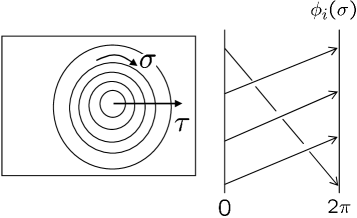
Figure 2: The string worldsheet coordinate. We map the coordinate from $(x_{0},x_{1})$ into $(\tau,\sigma)$.

Since multiple free closed strings can be regarded as a moduli space of this theory, one can consider a configuration with multiple strings of various length in general

$$\phi_{i}(\sigma^{a})=\phi_{i}(\sigma^{a}+2\pi w^{a})\ ,$$ (II.7)

where $n=\sum_{a=1}^{k}w^{a}$.

For our purpose, it is enough to analyze $U(2)$ gauge theory since the recombination is a local problem which involves two strings. At the tree level, the amplitude of this interaction is proportional to $g_{s}$. After the coordinate transformation (II.6), the action (II.5) is mapped into

$$S = -\frac{\theta}{8\pi g^{2}}\int d\tau d\sigma|z|^{2}$$ (II.8)

$${\rm tr}\left(2\left(\frac{\partial_{+}A_{-}}{z}-\frac{\partial_{-}A_{+}}{\bar{z}}-[A_{+},A_{-}]\right)^{2}\right.$$

$$+4\left(\frac{\partial_{+}\phi_{i}}{z}-[A_{+},\phi_{i}]\right)^{2}+[\phi_{i},\phi_{j}][\phi_{i},\phi_{j}]$$

$$\left.+2\bar{\psi}\Gamma^{+}\left(\frac{\partial_{+}\psi}{z}-[A_{+},\psi]\right)\right.$$

$$\left.+2\bar{\psi}\Gamma^{-}\left(\frac{\partial_{-}\psi}{\bar{z}}-[A_{-},\psi]\right)+2\bar{\psi}\Gamma_{i}[\phi_{i},\psi]\right)\ .$$

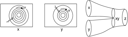
Figure 3: Two closed strings $x$ and $y$ recombine at some time and finally we obtain a single closed string $z$.

After the field redefinition :

$$A_{+}\to\frac{1}{z}\sqrt{\frac{g^{2}}{\theta}}A_{+}\ ,\quad A_{-}\to\frac{1}{\bar{z}}\sqrt{\frac{g^{2}}{\theta}}A_{-}\ ,$$

$$\psi_{R}\to\frac{1}{\sqrt{z}}\psi_{R},\quad\psi_{L}\to\frac{1}{\sqrt{\bar{z}}}\psi_{L}\ ,$$ (II.9)

and the rescaling :

$$\tau\to\sqrt{\frac{\theta}{g^{2}}}\tau\ ,\quad\sigma\to\sqrt{\frac{\theta}{g^{2}}}\sigma\ ,$$ (II.10)

we obtain the effective action

$$S = -\frac{\theta}{8\pi g^{2}}\int_{-\infty}^{\infty}d\tau\int_{0}^{2\pi w}d\sigma{\rm tr}\left(\frac{g^{2}}{\theta|z|^{2}}F^{2}_{z\bar{z}}+4D_{+}\phi_{i}D_{-}\phi_{i}\right.$$ (II.11)

$$+\frac{\theta|z|^{2}}{g^{2}}[\phi_{i},\phi_{j}][\phi_{i},\phi_{j}]+2\bar{\psi}(\Gamma^{+}D_{+}+\Gamma^{-}D_{-})\psi$$

$$\left.+2\sqrt{\frac{\theta}{g^{2}}}|z|\bar{\psi}\Gamma_{i}[\phi_{i},\psi]+O(\theta)\right)\ .$$

The parameter $\frac{g^{2}}{\theta}$ is identified with the string scale as $\alpha^{\prime}\equiv\frac{g^{2}}{\theta}$ in KN3 . $\phi_{i}$ has the target space dimension of $l_{s}$. Since the recombination is the local interaction, the length of the string does not affect the interaction. Thus, for simplicity, we can consider the two closed strings with the equal length. We parameterize the integral region of $\sigma$ as $[0,2\pi w]$.

This action is valid when two strings coincide in the target space. If two strings intersect at a point which is indeed the situation we consider in this paper, then the off-diagonal elements of this action are relevant only near the intersection point. They are meaningful only two strings are very close to each other since otherwise these modes become massive. Thus, we can describe off-diagonal modes as local fields $A^{12}_{\tilde{\mu}}(\tau,\sigma)$ which are valid near the intersection point with the small intersection angle.

The definitions of light-cone coordinates $\partial_{\pm}$ and $A_{\pm}$ are summarized in the appendix A.1. In the free string limit, we obtain light-cone Green-Schwarz superstring action which consists of marginal terms. In that case, every oscillator mode decomposes into a left mover and a right mover.

III Recombination

III.1 Fluctuation analysis and the recombination

In this section, by using the multiple closed superstring effective action (II.11) obtained in the previous section, we analyze the closed string interactions. In the IR limit, diagonal components are relevant degrees of freedom. Thus, the theory becomes a free theory in this limit. The leading interaction in the perturbative string theory is the interaction between two closed strings, which is realized as the recombination. The recombination can be investigated by using the Yang-Mills theory in HN which is introduced as the low energy effective action of D-strings.

Let us start from the two dimensional effective action (II.11). The Bosonic part is written as

$$S=-\frac{\theta}{8\pi g^{2}}\int_{-\infty}^{\infty}d\tau\int_{0}^{2\pi w}d\sigma{\rm tr}\left(\frac{g^{2}}{\theta|z|^{2}}F^{2}_{z\bar{z}}\right.$$

$$\left.+4D_{+}\phi_{i}D_{-}\phi_{i}+\frac{\theta|z|^{2}}{g^{2}}[\phi_{i},\phi_{j}][\phi_{i},\phi_{j}]\right)\ .$$ (III.1)

In KN3 , we identify the overall coefficient $\frac{\theta}{8\pi g^{2}}$ with $\frac{1}{8\pi\alpha^{\prime}}$ in the free string limit. Off-diagonal fields are regarded as local fields since we focus on the region where two strings are close to each other.

The string coupling is very weak in the IR region. On the analogy of matrix string theory DVV , the string coupling will behave $g_{s}\propto\frac{1}{|z|}$. We can interpret this relation as representing the equivalence between the IR limit and the weak coupling limit.

Supergravity solution of fundamental strings which is dual to our effective theory is described by IMSY

$$ds^{2} = \frac{U^{6}}{g_{\text{YM}}^{4}2^{7}\pi^{4}N}dx^{2}+\frac{1}{2\pi g_{\text{YM}}^{2}}dU^{2}+\frac{U^{2}}{2\pi g_{\text{YM}}^{2}}d\Omega^{2}\ ,$$

$$e^{\phi} = \left(\frac{g^{6}_{\text{YM}}2^{8}\pi^{5}N}{U^{6}}\right)^{-1/2}\ .$$ (III.2)

We can read the scaling behavior of $x$ as $x\sim 1/U^{3}$ from the metric. In the IR limit, the string coupling vanishes $e^{\phi}\sim U^{3}\sim 1/x\to 0$, which is consistent with our picture.

It seems that this kind of running coupling behavior makes it difficult to treat the interaction. However, the recombination happens at a definite scale. For simplicity, we fix the scale of $z$ as $|z|=z_{r}\equiv 1$ and treat this process in the real time. We map the coordinates from $z=e^{\tau+i\sigma}$ into $z=e^{i(t+\sigma)}$ by the analytic continuation $\tau\to it$. Then, the complex plane is mapped into the cylinder with the radius $|z|=1$. The Bosonic part of the action becomes

$$S=-\frac{\theta}{8\pi g^{2}}\int_{-\infty}^{\infty}dt\int_{0}^{2\pi w}d\sigma{\rm tr}\left(\frac{g^{2}}{\theta}F^{2}_{z\bar{z}}\right.$$

$$\left.+4D_{+}\phi_{i}D_{-}\phi_{i}+\frac{\theta}{g^{2}}[\phi_{i},\phi_{j}][\phi_{i},\phi_{j}]\right)\ .$$ (III.4)

This action is the two dimensional SU(2) Yang-Mills theory in the Lorentzian metric. Since we are considering the large winding number $w$, the worldsheet length of the string is very large. Thus, the solution of a single closed string might be represented locally as

$$\phi_{2} = \sqrt{\frac{g^{2}}{\theta}}\sigma\ ,$$

$$A_{\pm} = \psi=0,\quad\phi_{i}=0\ (i=3,\cdots,9)\ ,$$ (III.5)

in $U(1)$ gauge theory.

The solution which represents the intersecting strings is written as

$$(\phi_{2})_{\text{b.g.}} = \left(\begin{array}[]{cc}q\sqrt{\frac{g^{2}}{\theta}}\sigma&0\\ 0&-q\sqrt{\frac{g^{2}}{\theta}}\sigma\end{array}\right)=q\sqrt{\frac{g^{2}}{\theta}}\sigma\sigma^{3}\ ,$$ (III.8)

$$A_{\pm} = \psi=0,\quad\phi_{i}=0\ (i=3,\cdots,9)\ .$$ (III.9)

Two strings intersect at $\sigma=0$. Each string is connected with each other at a point far from the origin $\sigma=0$, which cannot be seen in this local solution near the intersection point. Thus, if the recombination occurs at this point, we obtain the single closed string. $q$ is a parameter which is related to the intersection angle $\phi$ as

$$q\equiv\tan\frac{\phi}{2}\ .$$ (III.10)

$q$ is the dimensionful quantity in the worldsheet sense and as we will see later, we relate it to the string coupling constant $g_{s}$. If we take $q\ll 1$, two strings are very close to each other in the target space, especially around the intersection point. Thus, our effective theory is valid.

We consider the fluctuations around this background. We turn on the fluctuations $a_{\pm}$ and $\varphi$

$$\phi_{2}=q\sqrt{\frac{g^{2}}{\theta}}\sigma\sigma^{3}+\sqrt{\frac{g^{2}}{\theta}}\varphi\sigma^{1},$$

$$A_{+}=a_{+}\sigma^{2}\ ,\quad A_{-}=a_{-}\sigma^{2}\ ,$$ (III.11)

since other fluctuations decouple from these fields at the quadratic level. $\sigma^{i}(i=1,2,3)$ are the Pauli matrices.

The quadratic lagrangian is obtained as

$$L =\frac{g^{2}}{\theta}\left[-(\partial_{+}a_{-}-\partial_{-}a_{+})^{2}\right.$$ (III.12)

$$-2(\partial_{+}\varphi-iqa_{+}\sigma)(\partial_{-}\varphi-iqa_{-}\sigma)$$

$$\left.-\sqrt{2}qa_{-}\varphi+\sqrt{2}qa_{+}\varphi\right]\ .$$

Note that these fluctuation terms do not come from $[\phi_{i},\phi_{j}][\phi_{i},\phi_{j}]$ terms. By choosing the gauge condition

$$a_{+}=-a_{-}\equiv\frac{a}{\sqrt{2}}\ ,$$ (III.13)

the quadratic lagrangian is written by the parameter $\tau$ and $\sigma$ as

$$L=\frac{g^{2}}{\theta}\left[(\partial_{t}a)^{2}+(\partial_{t}\varphi)^{2}-\left((\partial_{\sigma}\varphi)^{2}+2q\sigma a\partial_{\sigma}\varphi\right.\right.$$

$$\left.\left.+(qa\sigma)^{2}-2qa\varphi\right)\right]\ .$$ (III.14)

In order to solve the equation of motion for the fluctuations, we expand the fluctuations by the mass eigenfunctions

$$a(t,\sigma)=\sum_{n\geq 0}\tilde{a}(\sigma)C_{n}(t)\ ,$$

$$\varphi(t,\sigma)=\sum_{n\geq 0}\tilde{\varphi}(\sigma)C_{n}(t)\ ,$$ (III.15)

where $C_{n}(t)$ satisfy the equations

$$(\partial_{t}^{2}+m_{n}^{2})C_{n}(t)=0\ .$$ (III.16)

The differential equations are solved in the appendix B.1. For the lowest mode $n=0$, the eigenfunctions are calculated as

$$C_{0}(t) = C_{0}\cdot\exp(\sqrt{q}t)\ ,$$

$$\tilde{a}_{0}(\sigma) = \tilde{\varphi}_{0}(\sigma)=\exp\left(-\frac{q}{2}\sigma^{2}\right)\ ,$$ (III.17)

with the eigenvalue

$$m_{0}^{2}=-q\ .$$ (III.18)

These eigenfunctions are localized near the intersection point $\sigma\sim 0$. This mode is tachyonic and it causes the recombination HN .

III.2 The recombination probability

Since the transition probability from two strings into the single string depends on the string coupling constant $g_{s}$, we can identify $g_{s}$ by our investigation. We estimate the recombination probability per unit time. Since we put two strings with the relative center of mass velocity $v=0$ as the initial condition, the recombination always occurs if we wait long enough.

Before calculating the probability, we confirm that the lowest mode $C_{0}$ (from now on, we denote it as $C$) indeed causes the recombination. During and after the recombination, we investigate the time evolution of the tachyonic mode. Small fluctuations trigger the recombination and if we wait long enough, the recombination is over.

The recombination can be seen by the diagonalization of the background with the off-diagonal fluctuations

$$\phi_{2}(t,\sigma)=\frac{1}{2}\sqrt{\frac{g^{2}}{\theta}}\left(\begin{array}[]{cc}q\sigma&C(t)\tilde{\varphi}_{0}(\sigma)\\ C(t)\tilde{\varphi}_{0}(\sigma)&-q\sigma\end{array}\right)$$ (III.21)

$$\hskip 28.45274pt\xrightarrow{\text{diag}}\frac{1}{2}\sqrt{\frac{g^{2}}{\theta}}\times$$

$$\left(\begin{array}[]{cc}\sqrt{(q\sigma)^{2}+C^{2}(t)e^{-q\sigma^{2}}}&0\\ 0&-\sqrt{(q\sigma)^{2}+C^{2}(t)e^{-q\sigma^{2}}}\end{array}\right)\ .$$ (III.24)

(III.25)

Note that although this phenomenon locally represents the recombination of 2 strings $\to$ 2 strings, the final state is connected globally. Thus, this recombination represents the transition from two closed strings into the single closed string. We need to clarify the validity of the approximation since this geometrical picture comes from the fluctuation analysis. Our analysis is valid if the terms quadratic in the fluctuations are much smaller than the terms in the background. This condition is

$$(q\sigma)^{2}\gg C^{2}e^{-q\sigma^{2}}\ .$$ (III.26)

Since $q\sigma^{2}\sim O(1)$ as can be seen in (III.28), we obtain

$$q\gg C^{2}\ .$$ (III.27)

Our analysis is valid under this condition.

The action quadratic in the $C$ mode is obtained as

$$S=\frac{1}{8\pi}\int_{-\infty}^{\infty}dt\int_{-\pi w}^{\pi w}d\sigma\left((\partial_{t}C(t))^{2}+qC^{2}(t)\right)$$

$$\times\exp\left(-\frac{q}{2}\sigma^{2}\right)$$

$$\sim\frac{1}{8\pi}\sqrt{\frac{\pi}{2q}}\int_{-\infty}^{\infty}dt\left((\partial_{t}C(t))^{2}+qC^{2}(t)\right)\ .\hskip 5.69046pt$$ (III.28)

After integrating the $\sigma$ direction, this action can be regarded as a quantum mechanics of a particle moving in the inverse harmonic oscillator HH . As seen in (III.25), $C(t)$ is related to the separation of recombined strings. If $C$ takes a large value, then we can regard it as the signal for recombination. Once $C$ obtains the large value, the recombination is over. The separation of strings grows and finally we obtain a single closed string. In the inverse harmonic oscillator potential, the wave functions of the particle will keep spreading to the larger $|C|$. Thus, the recombination probability approaches 1 at $t\to\infty$.

The parameters in (III.28) can be interpreted in terms of the quantum mechanics of the particle moving in the inverse harmonic potential as

$$m \equiv \frac{1}{8\pi}\sqrt{\frac{\pi}{2q}}\ ,$$

$$\omega \equiv \sqrt{q}\ ,$$ (III.29)

where $m$ is the mass of the particle and $\omega$ is the frequency.

The Schrodinger equation is given by

$$i\frac{\partial\psi}{\partial t}=-\frac{1}{4m}\frac{\partial^{2}\psi}{\partial C^{2}}-m\omega^{2}C^{2}\psi\ .$$ (III.30)

As an initial condition at $t=0$, we consider the wave function to be a gaussian which is labeled by the parameter $\phi$. The derivation of the solution of the equation (III.30) is discussed in the appendix B.2. For large $t$, the wave function behaves

$$\psi(C,t)\sim(2/\pi)^{1/4}b^{-1/2}\exp\left(-\frac{1}{2}(\omega t+i\phi)\right)$$

$$\times\exp\left(-e^{-2\omega t}\frac{C^{2}}{b^{2}}+im\omega C^{2}\right)\ .$$ (III.31)

As discussed previously, once recombination happens, we obtain the single closed string as a final state. Since the fluctuation analysis is valid in the region $\sqrt{q}\gg C$, the geometric picture is also reliable in this region. We judge that the recombination has happened if the value of $C(t)$ grows beyond $\sqrt{q}=\omega$. Thus, the recombination probability at a time $t$ is estimated as

$$P(t) = 2\int_{\omega}^{\infty}dC|\psi(C,t)|^{2}$$ (III.32)

$$= 1-\text{Erf}(\sqrt{2}b^{-1}e^{-t\omega}\omega)$$

$$= 1-\text{Erf}\left(\sqrt{4m\omega^{3}\sin 2\phi}e^{-t\omega}\right)\ .$$

One can confirm that at $t\to\infty$, $P\to 1$. The recombination probability per unit time is calculated as

$$\frac{dP}{dt} = \frac{2}{\sqrt{\pi}}\sqrt{4m\omega^{5}\sin 2\phi}\exp\left(-4m\omega^{3}\sin 2\phi e^{-2t\omega}-t\omega\right)$$ (III.33)

$$= \frac{2^{1/4}}{\pi^{3/4}}q\sqrt{\sin 2\phi}$$

$$\times\exp\left(-\frac{q}{2\sqrt{2\pi}}\sin 2\phi e^{-2\sqrt{q}t}-\sqrt{q}t\right)\ .$$

In the small $q$ limit, the probability is proportional to

$$\frac{dP}{dt}\propto q\ .$$ (III.34)

In the perturbative string calculation, this probability is proportional to $g_{s}^{2}$. Thus, we identify

$$q\sim g_{s}^{2}\ .$$ (III.35)

The higher order corrections come from the expansion of the exponential function. By expanding this function at a time $t\sim O(\frac{1}{\sqrt{q}})$, and in the small $q$ limit, we obtain

$$\sum_{n=1}^{\infty}P_{n}q^{n}\ ,$$ (III.36)

which is consistent with the higher order corrections of the perturbative string if we identify $q$ with $g_{s}^{2}$ Polchinski ; JJP .

III.3 The recombination in matrix string theory

In this section, we estimate the recombination probability of intersecting strings from matrix string theory. The action of matrix string theory is written by the two dimensional Yang-Mills theory

$$S = \frac{1}{l_{s}^{2}}\int_{-\infty}^{\infty}d\tau\int_{0}^{2\pi w}d\sigma{\rm tr}\left((l_{s}^{2}g_{s}^{2})F^{2}_{z\bar{z}}\right.$$ (III.37)

$$+2(D^{+}\phi_{i}D_{+}\phi_{i}+D^{-}\phi_{i}D_{-}\phi_{i})$$

$$+\frac{1}{l_{s}^{2}g_{s}^{2}}[\phi_{i},\phi_{j}][\phi_{i},\phi_{j}]+2\bar{\psi}(\Gamma^{+}D_{+}+\Gamma^{-}D_{-})\psi$$

$$+\left.\frac{2}{g_{s}l_{s}}\bar{\psi}\Gamma_{i}[\phi_{i},\psi]\right)\ ,$$

where we consider long intersecting strings with the large winding number $w$. By the identification $\frac{\theta}{g^{2}}\equiv\frac{1}{l_{s}^{2}}$, the action (III.37) is very close to the action (III.4). The different point is the $g_{s}$ dependence which appears explicitly in (III.37). Thus, we perform the fluctuation analysis for the action (III.37) and investigate the $g_{s}$ dependence. Since the action is the same apart from the $g_{s}$ dependence, if we consider the same solution, we obtain the same tachyon mode as in section 3.1.

By regarding the tachyon effective action as the quantum mechanics of the particle moving in the inverse harmonic oscillator, the parameters $g_{s}$ and $q$ appear in the mass and frequency of the particle as

$$m \equiv \frac{g_{s}^{2}}{8\pi}\sqrt{\frac{\pi}{2q}}\ ,$$

$$\omega \equiv \sqrt{q}\ .$$ (III.38)

The only different point with respect to the analysis in section 3.1 is the $g_{s}$ dependence. The recombination probability at a time $t$ is estimated from the previous calculation (III.33) as

$$P(t)=1-\text{Erf}\left(\sqrt{4g_{s}^{2}\sqrt{\frac{\pi}{2}}q\sin 2\phi}e^{-\sqrt{q}t}\right)\ .$$ (III.39)

Thus, the recombination probability per unit time is

$$\frac{dP}{dt} = \frac{2^{1/4}}{\pi^{3/4}}g_{s}q\sqrt{\sin 2\phi}$$ (III.40)

$$\times \exp\left(-\frac{1}{2\sqrt{2\pi}}g_{s}^{2}q\sin 2\phi e^{-2t\sqrt{q}}-\sqrt{q}t\right)\ .\hskip 28.45274pt$$

By the rescaling

$$t\to g_{s}t\ ,$$ (III.41)

we obtain

$$\frac{dP}{dt} = \frac{2^{1/4}}{\pi^{3/4}}g_{s}^{2}q\sqrt{\sin 2\phi}$$ (III.42)

$$\times \exp\left(-\frac{g_{s}^{2}q}{2\sqrt{2\pi}}\sin 2\phi e^{-2g_{s}t\sqrt{q}}-\sqrt{q}g_{s}t\right)\ .\hskip 28.45274pt$$

This result is equivalent with the previous result (III.33) if we replace $q\leftrightarrow qg_{s}^{2}$. Thus, the identification we have derived in the section III.2 is consistent with matrix string theory.

At a large time $t\sim O(\frac{1}{g_{s}\sqrt{q}})$ in the small $q$ limit, the leading contribution is proportional to $g_{s}^{2}q$. The higher order corrections which come from the expansion of the exponential part are

$$(\text{leading contribution})\times\sum_{n=1}^{\infty}P_{n}g_{s}^{2n}\ ,$$ (III.43)

which is consistent with the perturbative string theory.

In BBN , the classical BPS solutions that interpolate between the initial and the final string configurations are constructed in matrix string theory. They interpret the amplitude of matrix string theory as the transition amplitude between initial and final configurations, and show that the leading contribution is proportional to $g_{s}^{-\chi}$ where $\chi$ is the Euler characteristic of the interpolating Riemann surface. Thus, they have reproduced the perturbative string amplitude from matrix string theory, which is consistent with our result.

IV Conclusion

We have identified the string coupling $g_{s}$ in IIB matrix model. We have constructed the classical solution of the strings in the action which is obtained from IIB matrix model. Starting from the configuration with the intersection angle $\phi=2\tan^{-1}q$ and no transverse distance and relative velocity, the recombination happens. This is triggered by the tachyonic fluctuations around the classical solution. After the recombination, we obtain the single closed string. We have estimated the probability of the recombination of two strings per unit time in this situation. The recombination probability is also calculated by the perturbative string theory. The leading contribution is proportional to $g_{s}^{2}$. The higher order corrections are seen as $\sum_{n=2}^{\infty}P_{n}g_{s}^{2n}$. Comparing our results with these behaviors, we have identified the string coupling $q\sim g_{s}^{2}$.

We have also estimated the recombination probability per unit time in the matrix string theory. The result shows the consistent behavior with that of the perturbative string theory. In the matrix string theory, the Yang-Mills coupling has the dimension $[length]^{-1}$ in the worldsheet and it is inversely proportional to the string coupling $g_{s}$. Thus, $g_{s}$ has the dimension $[length]$ in the worldsheet. Since $q$ has the worldsheet dimension $[length]^{-2}$, the dimensionless parameter is $qg_{s}^{2}$. Since the probability is the dimensionless quantity, $q$ should appear with $g_{s}^{2}$ which is consistent with the result obtained from IIB matrix model.

The parameter $q$ represents the ratio between the target space coordinate $\phi_{i}$ and the worldsheet coordinate $\sigma$. Another parameter which has this kind of property is the velocity $v$. Although the recombination probability depends on the relative velocity $v$, we have put $v=0$ in this paper. It might be interesting to calculate the probability of the recombination of intersecting strings with nonzero relative velocity.

Acknowledgments

This work is supported in part by the Grant-in-Aid for Scientific Research from the Ministry of Education, Science and Culture of Japan.

Appendix A Notation

A.1 Light-cone coordinates

$\partial_{\pm}$ are the derivatives with respect to

$$y_{\pm}\equiv\frac{1}{\sqrt{2}}(\tau\pm i\sigma)\ ,$$ (A.1)

and they are related to $\partial_{0}$ and $\partial_{1}$ as

$$\partial_{0}=\frac{1}{\sqrt{2}}(\frac{\partial_{+}}{z}+\frac{\partial_{-}}{\bar{z}})\ ,\quad\partial_{1}=\frac{i}{\sqrt{2}}(\frac{\partial_{+}}{z}-\frac{\partial_{-}}{\bar{z}}).$$ (A.2)

$A_{\pm}$ are related to $A_{0}$ and $A_{1}$ as

$$A_{0}=\frac{1}{\sqrt{2}}(A_{+}+A_{-})\ ,\quad A_{1}=\frac{i}{\sqrt{2}}(A_{+}-A_{-})\ .$$ (A.3)

The definition of $F_{z\bar{z}}$ in (II.11) is

$$F_{z\bar{z}} \equiv \bar{z}\partial_{+}(\bar{z}^{-1}A_{-})-z\partial_{-}(z^{-1}A_{+})-[A_{+},A_{-}]$$ (A.4)

$$= \partial_{+}A_{-}-\partial_{-}A_{+}-[A_{+},A_{-}]\ .$$

A.2 Pauli matrices

The Pauli matrices in (III.11) satisfy the following relation

$$[\sigma^{i},\sigma^{j}]=i\epsilon^{ijk}\sigma^{k}\ ,\quad{\rm tr}(\sigma^{i})^{2}=\frac{1}{2}\ .$$ (A.5)

Appendix B Calculation

B.1 The equation of motion for (III.14)

The derivation of the eigenfunctions (III.17) is summarized in this appendix.

By using the relation

$$\partial_{+}+\partial_{-} = -\sqrt{2}i\partial_{t}\ ,$$

$$2\partial_{+}\partial_{-} = -\partial_{t}^{2}+\partial_{\sigma}^{2}\ ,$$

$$\partial_{+}-\partial_{-} = -\sqrt{2}i\partial_{\sigma}\ ,$$ (B.1)

and imposing the gauge fixing condition $a_{+}=-a_{-}\equiv\frac{a}{\sqrt{2}}$, we obtain the lagrangian (III.14).

The equation of motion for the fluctuation lagrangian (III.14) is

$$\hat{O}\left(\begin{array}[]{c}a(t,\sigma)\\ \varphi(t,\sigma)\end{array}\right)=0\ ,$$ (B.4)

where

$$\hat{O}=\left(\begin{array}[]{cc}-(q\sigma)^{2}-\partial_{t}^{2}&-q\sigma\partial_{\sigma}+q\\ q\sigma\partial_{\sigma}+2q&-\partial_{t}^{2}+\partial_{\sigma}^{2}\end{array}\right)\ .$$ (B.7)

For the mass eigenvalues $m_{n}^{2}$ which satisfy the free field equation

$$(\partial_{t}^{2}+m_{n}^{2})C_{n}(\tau)=0\ ,$$ (B.8)

the equation of motion is given by

$$\left(\begin{array}[]{cc}-(q\sigma)^{2}+m_{n}^{2}&-q\sigma\partial_{\sigma}+q\\ q\sigma\partial_{\sigma}+2q&\partial_{\sigma}^{2}+m_{n}^{2}\end{array}\right)\left(\begin{array}[]{c}\tilde{a}(\sigma)\\ \tilde{\varphi}(\sigma)\end{array}\right)=0\ .$$ (B.13)

This differential equation is solved with the mass eigenvalue

$$m_{n}^{2}=(2n-1)q\ .$$ (B.14)

For the lowest mode $n=0$, the eigenfunctions are calculated as

$$C_{0}(\tau) = C_{0}\cdot\exp(\sqrt{q}t)\ ,$$

$$\tilde{a}_{0}(\sigma) = \tilde{\varphi}_{0}(\sigma)=\exp\left(-\frac{q}{2}\sigma^{2}\right)\ .$$ (B.15)

For general $n$, the eigenfunctions are

$$\tilde{a}_{n}(\sigma)= -e^{-\frac{q\sigma^{2}}{2}}\sum_{j=0,2,\cdots}^{n}(-1)^{\frac{j}{2}}\frac{4^{\frac{j}{2}}}{j!}\frac{n(n-2)\cdots(n-j+2)}{2n-1}$$

$$\times(j-1)\left(\sigma\sqrt{\frac{q}{2}}\right)^{j}\ ,$$

$$\tilde{\varphi}_{n}(\sigma)= e^{-\frac{q\sigma^{2}}{2}}\sum_{j=0,2,\cdots}^{n}(-1)^{\frac{j}{2}}\frac{4^{\frac{j}{2}}}{j!}\frac{n(n-2)\cdots(n-j+2)}{2n-1}$$ (B.16)

$$\times(2n\!-\!j\!-\!1)\left(\sigma\sqrt{\frac{q}{2}}\right)^{j}$$

for $n=0,2,\cdots$, and

$$\tilde{a}_{n}(\sigma)= -e^{-\frac{q\sigma^{2}}{2}}\sum_{j=1,3,\cdots}^{n}(-1)^{\frac{(j-1)}{2}}\frac{4^{\frac{(j-1)}{2}}}{j!}\left(\frac{j-1}{2}\right)$$

$$\times(n-3)\cdots(n-j+2)\left(\sigma\sqrt{\frac{q}{2}}\right)^{j}\ ,$$

$$\tilde{\varphi}_{n}(\sigma)= e^{-\frac{q\sigma^{2}}{2}}\sum_{j=1,3,\cdots}^{n}(-1)^{\frac{(j-1)}{2}}\frac{4^{\frac{(j-1)}{2}}}{j!}\left(n-\frac{j+1}{2}\right)$$ (B.17)

$$\times(n-3)\cdots(n-j+2)\left(\sigma\sqrt{\frac{q}{2}}\right)^{j}$$

for $n=3,5,\cdots$.

B.2 Solving the Schrodinger equation (III.30)

We summarize the derivation of the solution (III.31) in this appendix.

We describe the momentum conjugate to the $C$ as $\Pi$

$$\Pi=\frac{\delta L}{\delta\dot{C}}=2m\dot{C}\ .$$ (B.18)

Hamiltonian is given by

$$H = \Pi\dot{C}-L$$ (B.19)

$$= \frac{1}{4m}\Pi_{0}^{2}-m\omega^{2}C_{0}^{2}\ .$$

The Schrodinger equation (III.30) is solved by the wave function of the form

$$\psi(C,t)=A(t)\exp(-B(t)C^{2})\ ,$$ (B.20)

if $A$ and $B$ satisfy the equation

$$i\dot{A} = \frac{1}{2m}AB\ ,$$

$$\frac{i}{m}\dot{B} = \omega^{2}+\frac{1}{m^{2}}B^{2}\ .$$ (B.21)

These are solved in GP as

$$A = (2\pi)^{-1/4}\left(b\cos(\phi-i\omega t)\right)^{-1/2}\ ,$$

$$B = m\omega\tan(\phi-i\omega t)$$ (B.22)

$$= m\omega\frac{\sin 2\phi-i\sinh 2\omega t}{\cos 2\phi+\cosh 2\omega t}\ ,$$

where

$$a^{2} \equiv \frac{1}{2m\omega}\ ,$$

$$b = a(\sin 2\phi)^{-1/2}\ .$$ (B.23)

We put the initial condition of the wave function as

$$\psi(C,t=0)=(2\pi)^{-1/4}(b\cos\phi)^{-1/2}$$

$$\times\exp(-m\omega\tan\phi C^{2})\ .$$ (B.24)

The parameter $\phi$ controls the initial condition.

References

• (1) N. Ishibashi, H. Kawai, Y. Kitazawa and A. Tsuchiya, β€œA Large-N Reduced Model as Superstring,” Nucl. Phys. B498 (1997) 467, hep-th/9612115.
• (2) Y. Kitazawa and S. Nagaoka, β€œGreen-Schwarz superstring from type IIB matrix model,” Phys. Rev. D77 (2008) 026009, arXiv:0708.1077[hep-th].
• (3) R. Dijkgraaf, E. Verlinde and H. Verlinde, β€œMatrix String Theory,” Nucl. Phys. B500 (1997) 43, hep-th/9703030.
• (4) N. Itzhaki, J. M. Maldacena, J. Sonnenschein and S. Yankielowicz, β€œSupergravity and The Large N Limit of Theories With Sixteen Supercharges,” Phys. Rev. D58 (1998) 046004, hep-th/9802042.
• (5) Y. Kitazawa and S. Nagaoka, β€œSuperstring vertex operators in type IIB matrix model,” Phys. Rev. D77 (2008) 126016, arXiv:0710.0709[hep-th].
• (6) H. Kawai and M. Sato, β€œPerturbative Vacua from IIB Matrix Model,” arXiv:0708.1732[hep-th].
• (7) M. B. Green, J. H. Schwarz and L. Brink, β€œSuperfield Theory of Type II Superstrings,” Nucl. Phys. B219 (1983) 437.
• (8) A. Connes, M. Douglas and A. Schwarz, β€œNoncommutative Geometry and Matrix Theory: Compactification on Tori,” JHEP9802 (1998) 003, hep-th/9711162.
• (9) H. Aoki, N. Ishibashi, S. Iso, H. Kawai, Y. Kitazawa and T. Tada, β€œNon-commutative Yang-Mills in IIB Matrix Model,” Nucl. Phys. 565 (2000) 176, hep-th/9908141.
• (10) M. Li, β€œStrings from IIB Matrices,” Nucl. Phys. B499 (1997) 149, hep-th/9612222.
• (11) K. Hashimoto and S. Nagaoka, β€œRecombination of Intersecting D-branes by Local Tachyon Condensation,” JHEP 0306 (2003) 034, hep-th/0303204.
• (12) A. Hanany and K. Hashimoto, β€œReconnection of Colliding Cosmic Strings,” JHEP 0506 (2005) 021, hep-th/0501031.
• (13) J. Polchinski, β€œCollision Of Macroscopic Fundamental Strings,” Phys. Lett. B209 (1988) 252.
• (14) M. G. Jackson, N. T. Jones and J. Polchinski, β€œCollisions of Cosmic F- and D-strings,” JHEP 0510 (2005) 013, hep-th/0405229.
• (15) G. Bonelli, L. Bonora and F. Nesti, β€œString Interactions from Matrix String Theory,” Nucl. Phys. B538 (1999) 100, hep-th/9807232.
• (16) A. H. Guth and S.-Y. Pi, β€œThe Quantum Mechanics of the Scalar Field in the New Inflationary Universe,” Phys. Rev. D32 (1985) 1899.