Seeing Anderson Localization

Abstract

Anderson localization was discovered 50 years ago to describe the propagation of electrons in the presence of disorder Anderson58 . The main prediction back then, was the existence of disorder induced localized states, which do not conduct electricity. Many years later it turns out, that the concept of Anderson localization is much more general and applies to almost any type of propagation in time or space, when more than one parameter is relevant (like phase and amplitude). Here we propose a new optical scheme to literally see Anderson localization by varying the optical wavelength or angle of incidence to tune between localized and delocalized states. The occurrence of Anderson localization in the propagation of light, in particular, has become the focus of tremendous interest due to the emergence of new optical technologies and media, such as low dimensional and disordered optical lattices Schwartz07 ; Lahini08 . While several experiments have reported the measurement of Anderson localization of light Wiersma97 ; Berry97 ; Storzer06 ; Schwartz07 ; Lahini08 , many of the observations remain controversial because the effects of absorption and localization have a similar signature, i.e., exponential decrease of the transmission with the system size Scheffold99 ; Chabanov00 . In this work, we discuss a system, where we can clearly differentiate between absorption and localization effects because this system is equivalent to a perfect filter, only in the absence of any absorption. Indeed, only one wavelength is perfectly transmitted and all others are fully localized. These results were obtained by developing a new theoretical framework for the average optical transmission through disordered media.

In order to literally see Anderson localization, we consider the system shown in figure 1. The setup is composed of $N_{f}$ filters in series. Each filter is composed of $N_{l}$ random optical layers and each layer has a refractive index $n_{j}$ and a thickness $d_{j}$ as defined in figure 2. For optimal results, it is important that these layers are very well defined. This is possible, for instance, by using high accuracy multilayer growth techniques, such as molecular beam epitaxy (MBE). Good material choices include large band gap materials like GaN ($\Delta=3.2eV$, $n\simeq 2.3$) and InN ($\Delta=2eV$, $n\simeq 3.1$), which can be grown by MBE with atomic precision InN ; InN2 . The absence of any surface roughness ensures that this multilayered system is one-dimensional in nature. Surface roughness would induce scattering at stray angles, which leads to a 1D to 3D dimensional crossover Milner08 , thereby strongly reducing localization effects, since localization in 3D is much weaker than in 1D Abrahams79 and therefore much more challenging to observe Storzer06 .

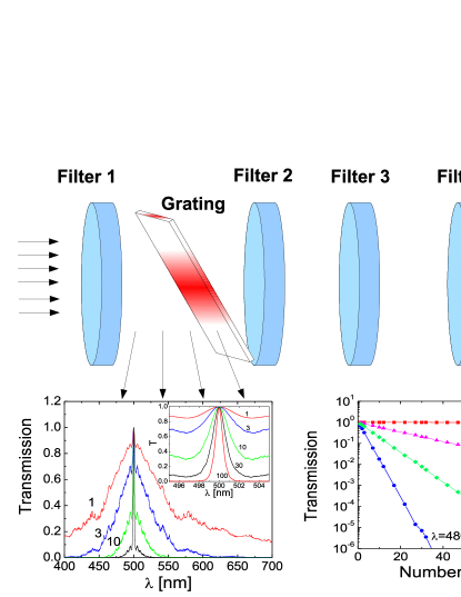
Figure 1: The top shows the arrangement of the filters, where a grating can be inserted in order to measure the wavelength dependence of the transmission. This transmission is shown in the bottom left figure when the grating is placed after 1, 3, 10, 30, or 100 filters, which increases the quality factor filter with the number of layers. The bottom right figure represents the dependence of the transmission on the number of layers at several wavelengths (480, 497, 499, and 500)nm, indicating an exponential decay

To illustrate the general behavior of our system, we considered the simplest random system, a binary distribution, where we assume two kinds of materials, one with a refraction index of $n_{0}=1$ and the other with $n_{1}=3$. Adding more materials will not change the results qualitatively and the analytical expressions derived below remain valid for any choice or combination of materials. However, to maximize the effect of disorder (smallest localization length) the variance of refraction indices should be largest. Since in most materials the refraction index rarely exceeds $n=3$, an efficient way to increase the variance is to consider a discrete distribution. Indeed, for a binary random distribution {$n_{0}=1$ and $n_{1}=3$} the variance is one as compared to a uniform random distribution $1\leq n\leq 3$, where the variance is reduced to one-third.

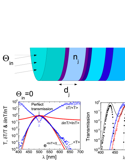
Figure 2: The top picture illustrates the details of a random sequence of layers composing one filter. In the bottom left figure the transmission as a function of wavelength is shown for a system of 200 layers averaged $10^{4}$ times. The analytical result from equation (3) is shown with a continuous line. The numerical average and relative fluctuations are shown with square and triangles. The transmission as a function of wavelength for different incidence angles (0, 15 and 30^∘) is depicted in the bottom right figure, where the continuous lines correspond to the analytical expression (3), whereas the dotted lines correspond to the numerical log-average.

The filters are placed in a way to allow the insertion of a grating between two of them. The grating is necessary to resolve the spectral composition of the transmitted light. The position of the grating can be changed in order to measure the transmission after 1, 2,…, or $N_{f}$ filters in series. When using a white light source, this allows to spectrally resolve the transmission after any number of filters. Anderson localization will then lead to an exponential decay of the transmission with the number of filters (see figure 1).

A major difficulty in observing Anderson localization is the existence of strong fluctuations Chabanov00 ; Genack05 . In general, the relative fluctuations of the transmission $(\delta T/\langle T\rangle)$ diverge with decreasing transmission, where $\delta T=\sqrt{(T-\langle T\rangle)^{2}}$ and $\langle T\rangle$ is the average transmission. This is a fundamental problem, which can be circumvented by considering $\ln(T)$ (the transmission in decibel) or the inverse transmission since in both cases the relative fluctuations decrease with decreasing transmission as shown in figure 2 for $\ln(T)$. Therefore, in order to reduce the fluctuations we can average the logarithm of the transmission over several disorder configurations, which converges much faster than an average over the transmission. The numerical examples shown in figure 1 are based on a small log-average over 100 configurations and assuming 100 different filters, each with an average of 50 random layers and a spectral resolution of 1nm. Such a log-average over a small number of configurations is feasible experimentally, since it simply involves averaging the signal in decibel over a few configurations. In comparison, a higher averaging is used in figure 2, where $10^{4}$ configurations with 200 random layers was used, leading to even less fluctuations. Considering a system of $N_{f}$ different filters allows one to perform a configurational average over the disorder, where the space between two filters is equivalent to an additional layer, as long as the distance between two filters follows the resonance condition described below. However, this is equivalent to simply considering a single filter with more random layers and then performing a configurational average, which is what we use in the remainder of this letter.

The results were obtained using a standard method to describe a multilayered optical system with a transfer matrix. Each matrix describes the transmission after one layer, where we assume the layers to be normal to the $\hat{x}$ direction. For TM (transverse magnetic) waves, where the magnetic field component $H^{z}$ is parallel to each layer and the electric field component $E^{y}$ is at an angle $\theta$ (the angle of incidence) to the first layer, the transfer matrix can be written as Chilwell84 :

$$\left(\begin{array}[]{c}H^{z}_{j-1}\\ E^{y}_{j-1}\end{array}\right)=\underbrace{\left(\begin{array}[]{cc}\cos(\phi_{j})&-i\sin(\phi_{j})/\gamma_{j}\\ -i\sin(\phi_{j})\gamma_{j}&\cos(\phi_{j})\end{array}\right)}_{M_{j}}\left(\begin{array}[]{c}H^{z}_{j}\\ E^{y}_{j}\end{array}\right),$$ (1)

For an incoming wave, of wavelength $\lambda$, the field components on one side of a stack of $N_{l}$ layers can therefore be related to the fields on the other side by taking the product of the transfer matrices ($M=\prod_{j=1}^{N_{l}}M_{j}$). Assuming a vacuum impedance $z_{0}$ before and after the filter, the transmission of light is given by $T=4|M_{11}+\gamma M_{12}+M_{21}/\gamma+M_{22}|^{-2}$, where $M_{kl}$ are the matrix elements of $M$ Chilwell84 . The matrix elements of $M_{j}$ used in equation (1) are material dependent with $\phi_{j}=(2\pi d_{j}/\lambda)\sqrt{n_{j}^{2}-\sin^{2}(\theta)}$ and $\gamma_{j}=(z_{0}/n_{j}^{2})\sqrt{n_{j}^{2}-\sin^{2}(\theta)}$. For TE (transverse electrical) waves these expressions have to be replaced by $H^{z}\rightarrow E^{z}$, $E^{y}\rightarrow-H^{y}$, and $\gamma_{j}=z_{0}^{-1}\sqrt{n_{j}^{2}-\sin^{2}(\theta)}$.

Absorption exists when the imaginary part of the refraction index is non-zero ($\Im\{n_{j}\}\neq 0$). $\Im\{n_{j}\}$ can be substantial when photon energies approach the band gap energy or when the materials are conducting. With absorption the localization-delocalization transition, described below, cannot be observed. For instance, for 100 layers and an imaginary part of the refraction index of only 0.01 the transmission at the resonance is decreased by about a factor 100 so that absorption effects can unambiguously be distinguished from localization effects. This is crucial, and in the remainder of this letter we will only consider the case without absorption, for which the localization-delocalization transition can be obtained under the following condition:

For a given layer there exists a set of thicknesses $d_{j}=m\lambda_{0}/2n_{j}$ ($m$ any integer) for which the layer is totally transparent at normal incidence and for the resonant wavelength $\lambda_{0}$. This corresponds to $\sin(\phi_{j})=0$ and to $M_{j}$ equal to the identity matrix. When randomly combining different layers with the same resonance condition, the overall resonance condition is preserved. The position of these resonances was discussed by Cristanti Crisanti90 . Away from the resonant wavelength the system behaves like a random system, leading to Anderson localization. This type of disorder was also studied in the context of electronic transport in 1D and 2D corr1 ; corr2 ; corr3 , where metal-insulator type transitions were found. Figures 1 and 2 show this resonance, where the transmission is one (transparent) at $\lambda_{0}=500$nm and then decreases exponentially ($T\simeq e^{-K(\lambda-\lambda_{0})^{2}}$) away from the resonance condition. $K$ is a form factor which is proportional to the number of random layers and also depends on the variance of the disorder as discussed below. This dependence on the number of layers can then be used to tune the quality factor of the filter. Without this special resonance condition, the transmission through random optical layers decays exponentially at all wavelengths Bouchaud86 ; Berry97 ; Bliokh04 .

We now turn to characterize the transmission through this random system by evaluating the product of $M_{j}$’s composed of random elements. Similar products of random matrices have been widely studied and lead to matrix elements, which increase exponentially with the number of products. The rate of this exponential dependence is termed the Lyapunov exponent and will be derived analytically below. The Lyapunov exponent also corresponds to the inverse of the localization length, beyond which the transmission vanishes. To obtain analytical results the trick is to consider the square of the fields, $|H^{z}_{j}|^{2}$ instead of $H^{z}_{j}$. This allows to concentrate on the dominant behavior beyond the plane wave oscillations. A similar technique was actually used in the context of electronic transport Erdos89 ; pendry94 ; Hilke08 and we extend it here to optical systems. Squaring equation (1) then leads to the following iterative equation:

$$\underbrace{\left(\begin{array}[]{c}|H^{z}_{j-1}|^{2}\\ |E^{y}_{j-1}|^{2}\\ 2\Im\{H^{z}_{j-1}(E^{y}_{j-1})^{*}\}\end{array}\right)}_{\vec{F}_{j-1}}=\underbrace{\left(\begin{array}[]{ccc}\cos^{2}(\phi_{j})&(\sin(\phi_{j})/\gamma_{j})^{2}&i\cos(\phi_{j})\sin(\phi_{j})/\gamma_{j}\\ (\sin(\phi_{j})\gamma_{j})^{2}&\cos^{2}(\phi_{j})&-i\cos(\phi_{j})\sin(\phi_{j})\gamma_{j}\\ 0&0&\cos^{2}(\phi_{j})-\sin^{2}(\phi_{j})\end{array}\right)}_{M^{3\times 3}_{j}}\underbrace{\left(\begin{array}[]{c}|H^{z}_{j}|^{2}\\ |E^{y}_{j}|^{2}\\ 2\Im\{(H^{z}_{j}(E^{y}_{j})^{*}\}\end{array}\right)}_{\vec{F}_{j}}.$$ (2)

For $N_{l}$ layers, the total transmission is now determined by the product $\vec{F_{0}}=(\prod_{j=1}^{N_{l}}M^{3\times 3}_{j})\vec{F}_{N_{l}}$, which can be averaged over the disorder, leading to, $\langle\vec{F_{0}}\rangle=\langle M^{3\times 3}\rangle^{N_{l}}\langle\vec{F_{N_{l}}}\rangle$, where $\langle M^{3\times 3}\rangle$ is the disorder average of $M^{3\times 3}_{j}$ assuming that the material parameters of the layers are not correlated. The disorder average depends on the distribution of the parameters entering $M^{3\times 3}_{j}$. The leading behavior is obtained by taking the eigenvalues of $\langle M^{3\times 3}\rangle$, from which the Lyapunov exponent can be extracted as $\Lambda=\max\{\ln|\mbox{Eig}(\langle M^{3\times 3}\rangle|)\}$. This yields an expression for the average resistance (inverse transmission), where $\langle 1/T\rangle=e^{\Lambda N_{l}}$. Hence, perfect transmission corresponds to the case where $\Lambda=0$. Interestingly, this expression can also be related to the log-average transmission $\langle\ln T\rangle=-\Lambda N_{l}/2$ and to the average transmission $\langle T\rangle=e^{-\Lambda N_{l}/4}$, where the factors of 1/2 stem from the properties of the distribution of $T$’s pendry94 . The next step is obtaining $\langle M^{3\times 3}\rangle$ for a given distribution. For discrete distributions, like the binary one this is quite straightforward, since the layer properties are determined by only two possible configurations, {$d_{0}$, $n_{0}$} and {$d_{1}$, $n_{1}$}, respectively. This yields

$$\langle M^{3\times 3}\rangle=(M^{3\times 3}_{0}+M^{3\times 3}_{1})/2,$$ (3)

where $M^{3\times 3}_{0}$ and $M^{3\times 3}_{1}$ are simply $M^{3\times 3}_{j}$ with {$d_{j}=d_{0}$, $n_{j}=n_{0}$ } and {$d_{j}=d_{1}$, $n_{j}=n_{1}$ }, respectively. For continuous distributions, analytical expressions for $\langle M^{3\times 3}\rangle$ are often too complicated to be useful and can be integrated numerically instead.

Comparing these analytical expressions to the numerical results demonstrate a remarkable agreement as seen in figures 1 and 2. The analytical expression using equation (3) reproduces all the main features and shows the resonance behavior at $\lambda=\lambda_{0}$. Evaluating the logarithm of the eigenvalues of expression (3) close to the resonance gives $\Lambda\sim(\lambda-\lambda_{0})^{2}$, which is perfectly reproduced by our numerical results and determines the form factor $K$, which depends on the variance of the disorder. (Zero variance leads to $K=0$ or $\Lambda=0$). Deviations exist when looking at the angle dependence, as shown in figure 2. While the analytical expression predicts two transmission peaks with a weak minimum in between, the numerical results show that the minimum is more pronounced. This can be attributed to restricting the average to the second moment, which can lead to differences with the numerical results and in some cases even lead to fluctuations in the Lyapunov exponent Hilke08 .

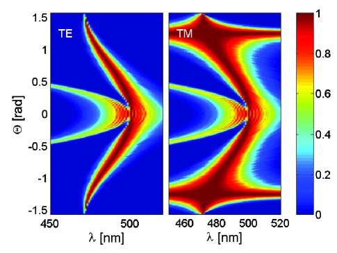
Figure 3: The wavelength and incidence angle dependence of the transmission through a random multilayer on a linear color scale for TE waves (left) and TM waves (right).

Quite remarkably, it is now possible to tune the wavelength of the resonance, simply by tilting the filter. We present the angle and wavelength dependence of the transmission in figure 3 for both the TE and TM waves using 200 random layers averaged over 100 configurations. Two branches can be observed, one which is perfectly transmitting and a second one which vanishes with increased angle. In addition, there is an angle $\Theta\simeq\pm 1.25$ with perfect transmission for the TM incidence, where $\Theta=\arctan(n_{1}/n_{0})$ rad and $n_{1}/n_{0}=3$ for our particular configuration. This angle corresponds to the Brewster angle.

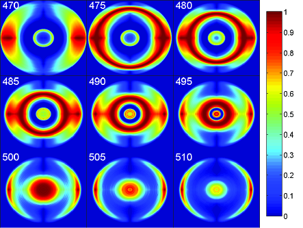
Figure 4: The transmission is shown on a linear color scale as a function of the angle of incidence in the $\hat{y}$ and $\hat{z}$ directions. Each subgraph spans -$\pi/2$ to +$\pi/2$ and corresponds to a different wavelength. The resonant wavelength ($\lambda_{0}=500nm$) corresponds to the bottom left panel. The horizontal (vertical) axis would correspond to the angle dependence of a TM (TE) wave.

By combining the expression for TE and TM waves it is possible to obtain the results for any polarization, simply by using a linear combination of TE and TM waves. Moreover, we can analyze what happens when tilting the filter in one or the other direction. The tilt angle can be varied in two spatial directions, one corresponding to the TM direction and the other to the TE direction, or a combination of both, which is seen in figure 4. Perfect transmission is now identified in a form of a ring, whose diameter depends on the wavelength. This angular dependence therefore allows for a direct and beautiful visualization of the localization-delocalization transition and hence of localization.

Summarizing, we have shown a new filter design, where we can directly visualize Anderson localization by using a localization-delocalization transition. The filter design is perfect in the sense that only one visible wavelength is transmitted perfectly and all others are exponentially suppressed. Not only does this provide for an optimal filter design but also allows us to see Anderson localization 50 years after its discovery.

References

- (1) Anderson, P. W. Absence of diffusion in certain random lattices. Phys. Rev. 109, 1492 1505 (1958)
- (2) Schwartz, T., Bartal, G., Fishman, S. & Segev, M. Transport and Anderson localization in disordered two-dimensional photonic lattices. Nature 446, 52 55 (2007)
- (3) Lahini, Y. et al. Anderson localization and nonlinearity in one-dimensional disordered photonic lattices. Phys. Rev. Lett. 100, 013906 (2008)
- (4) Wiersma, D. S., Bartolini, P., Lagendijk, A. & Righini, R. Localization of light in a disordered medium. Nature 390, 671 673 (1997)
- (5) Störzer, M., Gross, P., Aegerter, C. M. & Maret, G. Observation of the critical regime near Anderson localization of light. Phys. Rev. Lett. 96, 063904 (2006)
- (6) Berry, M. V. & Klein, S. Transparent mirrors: rays, waves and localization. Eur. J. Phys. 18, 222 228 (1997)
- (7) Scheffold, F., Lenke, R., Tweer, R. & Maret, G. Localization or classical diffusion of light? Nature 398, 206 270 (1999)
- (8) Chabanov, A. A., Stoytchev, M. & Genack, A. Z. Statistical signatures of photon localization. Nature 404, 850 853 (2000)
- (9) Ponce, F.A. & Bour, D.P. Nitride-based semiconductors for blue and green light-emitting devices. Nature 386, 351 - 359 (1997)
- (10) Khan, A., Balakrishnan, K & Katona, T. Ultraviolet light-emitting diodes based on group three nitrides. Nature Photonics 2, 77 - 84 (2008)
- (11) Milner, V., Zhang, S., Park, J. & Genack, A.Z. Photon Delocalization Transition in Dimensional Crossover in Layered Media. Physical Review Letters 101 183901 (2008)
- (12) Abrahams, E., Anderson, P. W., Licciardello, D. C. & Ramakrishnan, T. V. Scaling theory of localization: Absence of quantum diffusion in two dimensions. Phys. Rev. Lett. 42, 673 676 (1979)
- (13) Genack, A.Z. & Chabanov, A.A. Signatures of photon localization. J. Phys. A: Math. Gen. 38 10465-10488 (2005)
- (14) Chilwell, J. & Hodgkinson, I. Thin-films field-transfer matrix theory of planar multilayer waveguides and reflection from prism-loaded waveguides. J. Opt. Soc. Am. A 1, 742-753 (1984)
- (15) Crisanti, A. Resonances in random binary optical media. J. Phys. A: Math. Gen. 23 5235-5240 (1990)
- (16) Flores, J.C. Transport in models with correlated diagonal and off diagonal disorder. J. Phys. Condes. Matter., 1, 8471 (1989)
- (17) Dunlap, D.H., Wu, H.-L., & Phillips, P.W., Absence of localization in a random dimer model. Phys. Rev. Lett., 65, 88 (1990)
- (18) Hilke, M. Noninteracting Electrons and the Metal-Insulator Transition in Two Dimensions with Correlated Impurities. Phys. Rev. Lett., 91, 226403 (2003)
- (19) Bliokh, K.Yu. & Freilikher, V.D. Localization of transverse waves in randomly layered media at oblique incidence. Physical Review B 70 245121 (2004)
- (20) Bouchaud, J.P. & Le Doussal, P. Intermittency in random optical layers at total reflection. J. Phys. A: Math. Gen. 19 (1986) 797-810.
- (21) Erdos, P. & Herndon, R.R., Theories of electrons in one-dimensional disordered systems. Adv. Phys., 31, 65 (1982)
- (22) Pendry, J.B, Symmetry and transport of waves in 1D disordered systems. Adv. Phys., 43, 461 (1994)
- (23) Hilke, M. Ensemble-averaged conductance fluctuations in Anderson-localized systems. Phys. Rev. B 78, 012204 (2008)