Evolution of Magnetic Fields in High Mass Star Formation: SMA dust polarization image of the UCHII region G5.89-0.39

Abstract

We report high angular resolution (3$\arcsec$) Submillimeter Array (SMA) observations of the molecular cloud associated with the Ultra-Compact HII region G5.89-0.39. Imaged dust continuum emission at 870$\mu$m reveals significant linear polarization. The position angles (PAs) of the polarization vary enormously but smoothly in a region of 2$\times$10⁴ AU. Based on the distribution of the PAs and the associated structures, the polarized emission can be separated roughly into two components. The component ”x” is associated with a well defined dust ridge at 870 $\mu$m, and is likely tracing a compressed B field. The component ”o” is located at the periphery of the dust ridge and is probably from the original B field associated with a pre-existing extended structure. The global B field morphology in G5.89, as inferred from the PAs, is clearly disturbed by the expansion of the HII region and the molecular outflows. Using the Chandrasekhar-Fermi method, we estimate from the smoothness of the field structures that the B field strength in the plane of sky can be no more than 2$-$3 mG. We then compare the energy densities in the radiation, the B field, and the mechanical motions as deduced from the C¹⁷O 3-2 line emission. We conclude that the B field structures are already overwhelmed and dominated by the radiation, outflows, and turbulence from the newly formed massive stars.

1 Introduction

One of the main puzzles in the study of star formation is the low star formation efficiency in molecular clouds. Since molecular clouds are known to be cold, the thermal pressure is small. Hence, if there are no other supporting forces against gravity, the free-fall time scale will be short and the star formation rate will be much higher than what is observed. Magnetic (B) fields have been suggested to play the primary role in providing a supporting force to slow down the collapsing process (see the reviews by Shu et al. (1999) and Mouschovias & Ciolek (1999)). In these models, the B field is strong enough and has an orderly structure in the molecular cloud. The B field lines, which are anchored to the ionized particles, will then be dragged in along the direction of accretion, only when the ambipolar diffusion process allows the neutral component to slip pass the ionized component. In the standard low-mass star formation model (Galli & Shu 1993; Fiedler & Mouschovias 1993), an hourglass-like B field morphology is expected with an accreting disk near the center of the pinched field. Alternatively, turbulence has also been suggested as a viable source of support against contraction (see reviews by Mac Low & Klessen (2004) and Elmegreen & Scalo (2004)). The relative importance of B field and turbulence continues to be a hot topic as the two methods of support will lead to different scenarios for the star formation process.

Compared with the low mass stars, the formation process of high mass stars is really poorly understood. High mass star forming regions, because of their rarity, are usually at larger distances and are always located in dense and massive regions, because they are typically formed in a group. Hence, both poor resolution and complexity have hampered past observational studies. Furthermore, the environments of high mass star forming regions are very different from the low mass case because of higher radiation intensity, higher temperature, and stronger gravitational fields. Will the B fields in massive star forming sites have a similar morphology to the low mass cases?

Polarized emission from dust grains can be used to study the B field in dense regions, because the dust grains are not spherical in shape. They are thought to be aligned with their minor axes parallel to the B field in most of the cases, even if the alignment is not magnetic (Lazarian 2007). Due to the differences in the emitted light perpendicular and parallel to the direction of alignment, the observed thermal dust emission will be polarized, the direction of polarization is then perpendicular to the B field. Although the alignment mechanism of the dust grains has been a difficult topic for decades (see review by Lazarian 2007), the radiation torques seem to be a promising mechanism to align the dust grains with the B field (e.g., Draine & Weingartner 1996; Lazarian & Hoang 2007). However, other processes such as mechanical alignments by outflows can also be important.

Polarized dust emission has been detected successfully at arcsecond scales. The best example might be the low mass star forming region NGC 1333 IRAS 4A (Girart, Rao & Marrone 2006), which reveals the classic predicted hourglass B field morphology. Results on the massive star formation regions, such as W51 e1/e2 cores (Lai et al. 2001), NGC2024 FIR5 (Lai et al. 2002), DR21 (OH) (Lai et al. 2003), G30.79 FIR 10 (Cortes et al. 2006) and G34.4+0.23 MM (Cortes et al. 2008), typically show an organized and smooth B field morphology. However, this could be due to a lack of spatial resolution. Indeed, for the nearby high mass cases such as Orion KL (Rao et al. 1998) and NGC2071IR (Cortes, Crutcher, & Matthews 2006), abrupt changes of the polarization direction on small physical scales have been seen, which may suggest mechanical alignments by outflows as proposed by these authors. Whether high mass star forming regions will all show complicated B field structures on small scales remains to be examined.

In this study, we report on one of the first SMA measurements of dust polarization for a high mass star forming region, G5.89-0.39 (hereafter, G5.89). The linearly polarized thermal dust emission is used to map the B field at $\sim$3$\arcsec$ resolution, and the C¹⁷O 3-2 line is used to study the structure and kinematics of the dense molecular cloud. The description of the source, the observations and the data analysis, the results, and the discussion are in Sec. 2, 3, 4 and 5, respectively. The conclusions and summary are in Sec. 6.

2 Source Description

G5.89 is a shell-like ultracompact HII (UCHII) region (Wood et al. 1989) at a distance of 2 kpc (Acord et al. 1998). The UCHII region is 0.01 pc in size, and its dynamical age is 600 years, estimated from the expansion velocity (Acord et al. 1998). Observations of the K_s and $L^{\prime}$ magnitudes and color by Feldt et al. (2003) suggest that G5.89 contains an O5 V star.

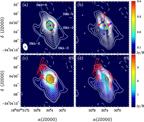
Figure 1: (a) The SMA 870 $\mu$m total continuum image (contours) overlayed on the VLA 2cm continuum (free-free continuum; color scale). The white contours represent the continuum emission strength at 3, 5, 10, 15, 20, 25 … 60 and 65 $\sigma$ levels, and the black contours in the center represent 70, 80, 90, 100 and 110 $\sigma$ levels, where $1\sigma$ is 30 mJy Beam^-1. The star marks the O star detected by Feldt et al. (2003). The asterisk marks the origin of the Br$\gamma$ outflow detected by Puga et al. (2006). The SMA and VLA synthesized beams are shown as white and black ellipses at the lower-left corner, respectively. The white ”+” mark the positions of the sub-mm peaks identified in Hunter et al. (2008). (b) The same as in (a), with the white contours representing the SMA 870 $\mu$m dust continuum (after the subtraction of the free-free continuum). The contours start from and step in $3\sigma$, where $1\sigma$ is 30 mJy Beam^-1. The color wedge on the upper-right edge represents the strength of the 2cm free-free continuum in the units of Jy Beam ^-1. The red and blue arrows indicate the axes of the molecular outflows. The outflows in the N-S and NW-SW direction in the west of O5 star are identified in Hunter et al. (2008). The 3rd outflow in the east of O5 star is identified in Tang et al. (in prep.). (c) The polarization (red segments) derived by using image (a). The length of the red segment represents the percentage of the polarized intensity. The 870 $\mu$m continuum is shown both in white contours with the steps as in Fig. (a) and in the color scale. (d) The polarization (red segments) derived by using image (b). The 870 $\mu$m dust continuum is again shown both in white contours with the steps as in Fig. (b) and in the color scale. The color wedge at the lower-right edge shows the strength of the dust continuum in the units of Jy Beam^-1. In (c) and (d), the polarization plotted is above 3$\sigma_{I_{p}}$.

Just as in other cases of massive stars, G5.89 contains most likely a cluster of stars. The detections of associated H₂O masers (Hofner & Churchwell 1996), OH masers (Stark et al. 2007; Fish et al. 2005) and class I CH₃OH masers (Kurtz et al. 2004), suggest that multiple stars have formed in this region. Furthermore, the morphology of the detected molecular outflows also suggest the presence of multiple driving sources, because different orientations are observed in different tracers. In CO 1-0, the large scale outflow is almost in the east-west direction (Harvey & Forveille 1988; Watson et al. 2007). In C³⁴S and the OH masers, the outflow is in the north-south direction (Cesaroni et al. 1991; Zijlstra et al. 1990). In SiO 5$-$4, the outflow is at a position angle (PA) of 28$\arcdeg$ (Sollins et al. 2004). In the CO 3-2 line, the outflows (Hunter et al. 2008) are in the north-south direction and at the PA of 131$\arcdeg$, and the latter one is associated with the Br$\gamma$ outflow (Puga et al. 2006). In addition, the detected 870 $\mu$m emission has also been resolved into multiple peaks (labelled in Fig. 1(a); Hunter et al. 2008). The different masers, the multiple outflows, and the multiple dust peaks, are all consistent with the formation of a cluster of young stars.

G5.89 should be expected to have a substantial impact on its environment. In terms of the total energy in outflows in this region, G5.89 is definitely one of the most powerful groups of outflows ever detected (Churchwell 1997).

3 Observation and Data Analysis

The observations were carried out on July 27, 2006 and September 10, 2006 using the Submillimeter Array (Ho, Moran & Lo (2004)) in the compact configuration, with 7 of the 8 antennas available for both tracks. The projected lengths of the baselines ranged from 6.5 to 70 k$\lambda$ ($\lambda\approx$870$\mu$m). Therefore, our observational results are insensitive to structures larger than 39$\arcsec$. The SMA receivers are intrinsically linearly polarized and only one polarization is available at the current time. Thus, quarter-wave plates (see Marrone & Rao 2008) were installed in order to convert the linear polarization (LP) to circular polarization (CP). The quarter-wave plates were rotated by 90$\arcdeg$ on a 5 minutes cycle using a Walsh function to switch between 16 steps in order to sample all the 4 Stokes parameters. The integration time spent on the source in each step was approximately 15 seconds. The overhead required in switching between the different states was approximately 5 seconds. In each cycle all four cross-correlations (LL, LR, RL, and RR) were each calculated 4 times. The data were then averaged over this complete cycle in order to obtain quasi simultaneous dual polarization visibilities. We assume that the smearing due to the change of the polarization angles on this time scale is negligible.

The local oscillator frequency was tuned to 341.482 GHz. With a 2 GHz bandwidth in each sideband we were able to cover the frequency range from 345.5 to 347.5 GHz and from 335.5 to 337.5 GHz in the upper and lower sideband, respectively. The correlator was set to a uniform frequency resolution of 0.65 MHz ($\sim$ 0.7 km s^-1) for both sidebands. While our main emphasis was to map the polarized continuum emission from the dust, we were also able to detect a number of molecular lines simultaneously. These results will be published separately.

Generally, the conversions of the LP to CP of the receivers are not perfect. This non-ideal characteristic of the receiver will cause an unpolarized source to appear polarized, which is known as instrumental polarization or leakage. Nevertheless, these leakage terms (see Sault, Hamaker, & Bregman 1996) can be calibrated by observing a strong linearly polarized quasar. In this study, the leakage and bandpass were calibrated by observing 3c279 for the first track and 3c454.3 for the second track. Both sources were observed for 2 hours while they were transiting in order to get the best coverage of parallactic angles. The leakage terms are frequency dependent, $\sim$1% and $\sim$3% for the upper and lower sideband before the calibration, respectively. After calibration, the leakage is less than 0.5$\%$ in both sidebands. Besides the calibration for the polarization leakage, the amplitudes and phases were calibrated by observing the quasars 1626-298 and 1924-292 every 18 minutes. These two gain calibrators in both tracks were used because of the availabilities of the calibrators during the observations. Finally, the absolute flux scale was calibrated using Callisto.

The data were calibrated and analyzed using the MIRIAD package (Sault, Teuben, & Wright 1995). After the standard gain calibration, self-calibration was also performed by selecting the visibilities of G5.89 with uv distances longer than 30 k$\lambda$. As a result, the sidelobes and the noise level of the Stokes $I$ image were reduced by a factor of 2. In order to get the images from the measured visibilities, the task INVERT in the MIRIAD package was used. The Stokes $Q$ and $U$ maps are crucial for the derivation of the polarization segments. We used the dirty maps of $Q$ and $U$ to derive the polarization to avoid a possible bias introduced from the CLEAN process. The Stokes $I$ map shown in this paper is after CLEAN.

The Stokes $I$, $Q$ and $U$ images of the continuum were constructed with natural weighting in order to get a better S/N ratio for the polarization. The final synthesized beam is $3\arcsec.0\times 1\arcsec.9$ with the natural weighting. The C¹⁷O images are presented with a robust weighting 0.5 in order to get a higher angular resolution, and the synthesized beam is 2.8$\arcsec\times$1.8$\arcsec$ with PA of 13$\arcdeg$. The noise levels of the $I$, $Q$ and $U$ images are $\sim$ 30, 5 and 5 mJy Beam^-1, respectively. Note that the noise level of the Stokes $I$ image is much larger than the ones in the Stokes $Q$ and $U$ images. The large noise level of the $I$ image is most likely due to the extended structure, which can not be recovered with our limited and incomplete uv sampling. The strength (I_p) and percentage ($P$) of the linearly polarized emission is calculated from: $I_{p}^{2}=Q^{2}+U^{2}-\sigma_{Q,U}^{2}$ and $P$ = I_p/I, respectively. The term $\sigma_{Q,U}$ is the noise level of the Stokes $Q$ and $U$ images, and it is the bias correction due to the positive measure of I_p. The noise of I_p ($\sigma_{I_{p}}$) is thus 5 mJy Beam^-1. The presented polarization is derived using the task IMPOL in the MIRIAD package, where the bias correction of $\sigma_{I_{p}}$ is included.

4 Results

In this section, we present the observational results of the dust continuum and the dust polarization at 870$\mu$m, and the C¹⁷O 3-2 emission line. No polarization was detected in the CO 3-2 emission line.

4.1 Continuum Emission

The total continuum emission at 870 $\mu$m, shown in Fig. 1(a), is resolved with a total integrated flux density 12.6$\pm$1.3 Jy. In general, the morphology of the continuum emission at 870$\mu$m is similar to the emission at 1.3 mm by Sollins et al. (2004). However, the 870$\mu$m emission peaks at $\sim$ 1$\arcsec$ west of the position of the O5 star, which is offset toward the north-west by $\sim$1$\arcsec$.7 from the peak of the 1.3 mm continuum emission. Because there is still a significant contribution from the free-free emission to the continuum at 870 $\mu$m and at 1.3mm, the differences between the 870 $\mu$m and 1.3 mm maps most likely result from the increasing contribution from the dust emission as compared to the free-free emission at shorter wavelengths. Due to the importance of a correct dust continuum image in the derivation of the polarization, we describe here how the free-free continuum was estimated and removed from the 870$\mu$m total continuum emission.

4.1.1 Removing the free-free emission

The free-free continuum at 2cm (shown in color scale in Fig.1 (a) and (b)) was imaged from the VLA archival database observed on August 7, 1986. The VLA synthesized beam of the 2cm free-free image is 0$\arcsec.92\times$0$\arcsec$.45 with natural weighting of the uv data. Since the free-free shell is expanding at a rate of 2.5 mas year^-1 (Acord et al. 1998), at a distance of 2 kpc, this expansion motion over the intervening 20 years is negligible within the synthesized beam of our SMA observation.

The contribution from the free-free continuum was removed by the following steps. Firstly, we adopted a spectral index $\alpha=-$0.154 calculated in Hunter et al. (2008) for the free-free continuum emission between 2cm to 870$\mu$m. The resulting estimated free-free continuum strength at 870$\mu$m was 4.9 Jy. Secondly, we further assumed that the morphology of the free-free continuum at 870 $\mu$m and at 2cm were identical. We then smoothed the VLA 2cm image to the SMA resolution and scaled the total flux density to 4.9 Jy. Finally, we subtracted this image from the total continuum at 870 $\mu$m. The resultant 870 $\mu$m dust continuum image is shown in Fig. 1(b). The total flux density of the dust continuum is therefore 7.7$\pm$0.8 Jy.

4.1.2 Dust continuum: mass and morphology

The corresponding gas mass (M_gas) was calculated from the flux density of the dust continuum at 870 $\mu$m following Lis et al. (1998):

$$M_{gas}=\frac{2\lambda^{3}Ra\rho d^{2}}{3hcQ(\lambda)J(\lambda,T_{d})}S(\lambda)$$ (1)

Here, we assumed a gas-to-dust mass ratio $R$ of 100, a grain radius $a$ of 0.1 $\mu$m, a mean grain mass density $\rho$ of 3 g cm^-3, a distance to the source $d$ of 2 kpc, a dust temperature $T_{d}$ of 44 K, an observed flux density S$(\lambda)$ of 7.7 Jy, the Planck factor $J(\lambda,T_{d})=[exp(hc/\lambda kT_{d})-1]^{-1}$. $h$, $c$ and $k$ are the Planck constant, the speed of light and the Boltzmann constant, respectively. The grain emissivity $Q$($\lambda$) was estimated to be $1.5\times 10^{-5}$ after assuming $Q(350\mu m)$ of $7.5\times 10^{-4}$ and $\beta$ of 2 (cold dust component), and using the relation $Q(\lambda)=Q(350\mu m)(350\mu m/\lambda)^{\beta}$ (Hunter et al. 2000). As suggested in the same paper, the dust emission can be modeled by two temperature components, with the emission dominated by the colder component at T_d $\sim$ 44 K. We adopted this value for T_d, and therefore, the mass given here refers only to the cold component and is an underestimate of the total mass. The derived gas mass of the dust core M_gas is $\sim$ 300 M_☉, with a number density $n_{H_{2}}=$ 5.3$\times$10⁶ cm^-3 averaged over the emission region. The sizescale along the line of sight is assumed to be 0.13 pc, which is the diameter of the circle with the equivalent emission area.

The dust emission presented in Fig. 1(b) has an extension toward the northeast, east and southwest and has a steep roll off on the northwestern edge of the ridge. In the higher angular resolution (0.8$\arcsec$) observation at the same wavelength by Hunter et al. (2008), the dust core is resolved into 5 peaks, where the two strongest peaks align in the north-south direction to the west of the O5 star. The dust continuum emission associated with SMA-N, SMA-1 and SMA-2 is called sharp dust ridge hereafter because of its strong emission and its morphology. There is no peak detected at the position of the O5 star. It is likely that the O5 star is located in a dust-free cavity, as proposed by Feldt et al. (1999) and Hunter et al. (2008).

4.2 Dust polarization

We first compare the dust polarization derived from the 870 $\mu$m total continuum (Fig. 1(c)) and from the 870 $\mu$m dust continuum (Fig. 1(d)). In both cases the derived polarization is at the same location with the same PAs. The only difference of the polarization in Fig. 1(c) and 1(d) is that the percentage of polarization near the HII region is increased in Fig. 1(d). This is because of the fact that the free-free continuum is not polarized, and the $Q$ and $U$ components are not affected by the free-free continuum subtraction. Therefore, the expected polarization percentage will increase when the free-free continuum is removed from the 870 $\mu$m continuum. The total detected polarized intensity I_p is 59 mJy. All the polarization shown in the figures besides Fig. 1(c) is calculated from the derived dust continuum image. The off-set positions, percentages and PAs of the polarization segments are listed in Table 1.

4.2.1 Morphology of the detected polarization

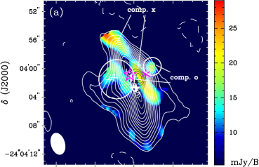
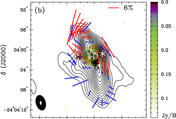
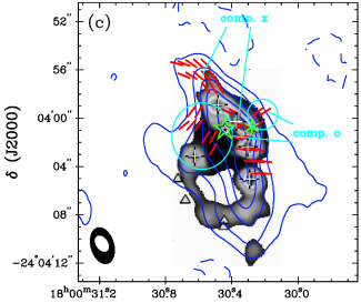
Figure 2: (a) The 870$\mu$m dust continuum (white and grey contours) overlaid on the polarized intensity (I_P) image (color scale). The contours plotted are the same as in Fig. 1(b). The color wedge shows the strength of polarization intensity in units of mJy Beam^-1. The smallest white open circles and plus signs mark the positions of the Zeeman pairs of the OH maser (Stark et al. 2007) with different polarimetries. The other symbols are the same as in Fig. 1. The larger solid white circles mark component ”o”, defined in Sec. 4.2.2. (b) The polarization (red and blue segments) overlaid on the 870 $\mu$m dust continuum (black contours) and the 2cm free-free continuum emission (color scale). In red and blue segments are polarization segments above 3$\sigma_{I_{p}}$ and between 2 to 3$\sigma_{I_{p}}$, respectively. The contours, star, asterisk, circles and plus signs are all the same as in (a). The color wedge shows the strength of the 2cm free-free emission in units of Jy Beam^-1. The ellipses in the lower-left corner are the synthesized beams of this paper, shown in black, and of the 2cm free-free continuum image, shown in white. (c) The inferred B field (red segments) overlaid on the 870 $\mu$m dust continuum (blue contours) in this paper and in Hunter et al. (2008) (grey scale). The ellipses in the lower-left corner are the synthesized beams of this work, shown in black, and of Hunter et al. (2008), shown in white. The white crosses mark the sub-mm sources detected by Hunter et al. (2008). The triangles mark the positions of the H₂ knots identified in Puga et al. (2006).

The polarized emission is not uniformly distributed. Detected polarization at 2$\sigma_{I_{p}}$ are shown as blue segments and detections above 3$\sigma_{I_{p}}$ are shown by red segments. Most of the polarized emission is located in the northern half of the dust core close to the HII region and appears as 4 patches, mostly with $\sigma_{I_{p}}\geq 3$ (Fig. 2(a) in color scale). There is a sharp gap where no polarization is detected extending from the NE to the SW across the O star. The southern half of the dust core is free of polarization, except for a few positions at the edge of the dust core. However, the polarization in the south half of the dust core is at 2 to 3$\sigma_{I_{p}}$ level only. We will focus our discussions on the more significant detections in the core of the cloud.

We separate the polarized emission into two groups. We are guided principally by the fact that one group is associated with the periphery of the total dust emission, while the other group tracks the strongest parts of the total dust emission. The polarized patches to the east of the O star and to the west of the Br$\gamma$ outflow source have similar PAs of $\sim 50\arcdeg$ (Fig. 2(b)). These polarization segments are located at the fainter edges of the higher resolution 870 $\mu$m dust continuum image (Fig. 2(c); Hunter et al. 2008) and at the less steep part of the 3$\arcsec$ resolution image (this paper). This may suggest that this polarization originates from a more extended overall structure, rather than from the detected condensations. Therefore, these polarization segments are suggested to be the component ”o” (defined in the next section). The rest of the polarization in the northern part is all next to the sharp gap where no polarization is detected. Most of the polarization is on the 870$\mu$m sharp dust ridge observed with 0.8$\arcsec$ resolution, except for the ones at the NE and SW ends where the polarization patches stretch toward the extended structure. At these NE and SW ends the polarization is probably the sum of the extended and the condensed structures. These polarization segments are suggested to belong to the component ”x”.

The 0.8$\arcsec$ resolution observations show that there is a hole in the southern part of the detected dust continuum. This hole is not resolved with the 3$\arcsec$ synthesized beam of our map. That may explain why polarization is not detected at this position. Here, and also for the dust ridge sharply defined with 0.8$\arcsec$ resolution, the dust polarization is sensitive to the underlying structures and can help to identify unresolved features which are smaller than our resolution.

4.2.2 Distribution of the polarization segments

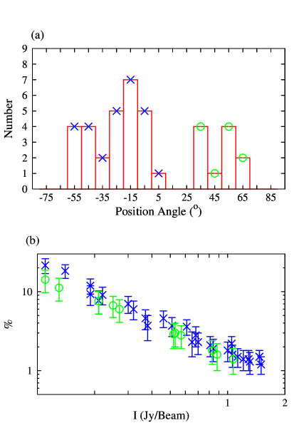
Figure 3: (a) Distribution of the PAs (defined in the range $-$90$\arcdeg$ to 90$\arcdeg$) of the polarization in G5.89. (b) Total intensity (I) versus percentage (%) of the polarized flux density. In both (a) and (b) panels, the statistics are from the detected polarization segments above 3 $\sigma_{I_{p}}$ confidence level. The ”cross” represents the component ”x”, which is associated with the sharp dust ridge. The ”circle” represents the component ”o”, which is associated with the extended structure.

The detected PAs vary enormously over the entire map, ranging from $-60\arcdeg$ to 61$\arcdeg$ (Fig. 3(a)). Nevertheless, they vary smoothly along the dust ridge and show organized patches. We have roughly separated the polarized emission into two different components according to their locations (as discussed in Sec. 4.2.1) and their PAs. The ”o” component is probably from an extended structure with PAs ranging from 33$\arcdeg$ to 61 $\arcdeg$. The mean PA weighted with the observational uncertainties of component ”o” is 49$\pm$3$\arcdeg$, with a standard deviation of 11$\arcdeg$. The ”x” component associated with the sharp dust ridge has PAs ranging from $-60\arcdeg$ to 4$\arcdeg$. Its weighted mean PA is $-$24$\pm$1$\arcdeg$, with a standard deviation of 18$\arcdeg$. If the polarization were not separated into two components, the weighted mean PA is $-$9$\arcdeg$ with a standard deviation of 39$\arcdeg$.

The relation between the percentage of polarization and the intensity is shown in Fig. 3(b). The percentage of polarization decreases towards the denser regions, which has already been seen for other star formation sites, such as the ones listed in Sec. 1. This is possibly due to a decreasing alignment efficiency in high density regions, because the radiation torques are relatively ineffective (Lazarian & Hoang 2007). It can also be due to the geometrical effects, such as differences in the viewing angles (Gonçalves et al. 2005), or due to the results from averaging over a more complicated underlying field morphology.

4.3 C¹⁷O 3-2 emission line

In order to trace the physical environments and the gas kinematics in G5.89, we choose to use the C¹⁷O 3-2 emission line because of its relatively simple chemistry. The critical density of C¹⁷O 3-2 is $\sim$ 10⁵ (cm^-3), assuming a cross-section of 10^-16 (cm^-2) and a velocity of 1 km s^-1, and therefore, it will trace both the relative lower (n${}_{H_{2}}$ $\sim$10⁵ (cm^-3)) and higher (n${}_{H_{2}}$$\sim$ 10⁶ (cm^-3)) density regions. Although its critical density is much smaller than the estimated gas density of 5.3$\times$10⁶ (cm^-3) from the dust continuum, it is apparently tracing the same regions as the dust continuum because of the similar morphology of the integrated intensity image, shown in the next section. We therefore assume that the kinematics traced by C¹⁷O represents the bulk majority of the molecular cloud and that it is well correlated with the dust continuum.

4.3.1 Morphology of C¹⁷O 3-2 emission

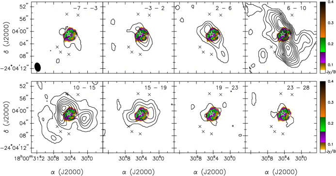
Figure 4: The C¹⁷O 3-2 line emission (black contours) integrated in 8 different velocity ranges, as indicated in each panel in units of km s^-1. The color scale images represent the VLA 2cm free-free continuum emission with its strength shown in the wedge in units of Jy Beam^-1. To show the fainter component in the higher velocity panels, the black contours represent the strengths at 2,6,10,15,21,27,33,40,48 $\sigma$, where 1 $\sigma$ is 0.4 Jy Beam^-1 km s^-1. The black crosses mark the positions of the H₂ knots detected by Puga et al. (2006). The other symbols are the same as in Fig. 1. In the panels from $-$7 to $-$3 and 23 to 28 km s^-1, the C¹⁷O dense cloud has an extension similar to the dust ridge detected in the 0.8$\arcsec$ dust continuum image (Fig. 2). The peak positions of the high velocity components do not coincide with the location of the O5 star.

The emission of the C¹⁷O 3-2 line covers a large velocity range, from $-$7 to 28 km s^-1, as shown in the channel maps in Fig. 4. The majority of the gas traced by the C¹⁷O 3-2 line is relatively quiescent and has a morphology similar to the 870$\mu$m dust continuum emission. Besides the components which trace the dust continuum, an arc feature is seen in the south-east corner of the panel covering 10 to 15 km s^-1. There is no associated 870$\mu$m dust continuum detected at this location, probably due to the low total column density or mass of this feature. Another feature seen in the more quiescent gas is the clump extending towards the south of the dust core (see the panel covering 6 to 10 km s^-1 in Fig. 4). This clump has a similar morphology as seen in the 870 $\mu$m dust continuum where no polarization has been found. At the higher velocity ends, i.e. from $-$7 to $-$3 km s^-1 and from 23 to 28 km s^-1, the emission appears at the 870$\mu$m dust ridge. This suggests that at the sharp dust ridge, there are high velocity components besides the majority of quiescent material. Furthermore, the brightest HII features appear correlated with the strongest C¹⁷O emission, especially at low velocities (v${}_{lsr}=$ 6 to 15 km s^-1), which may point toward an interaction between the molecular gas and the HII region.

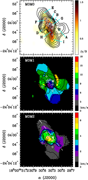
Figure 5: Upper Panel: The total integrated intensity (0th moment) image of the C¹⁷O 3-2 emission line (black contours) overlaid on the dust continuum at 870 $\mu$m (color scale). The contours represent the emission strength starting from and stepping in 3 Jy Beam^-1 km s^-1. The letters mark the positions where the spectra were taken in Fig. 7. The black cross marks the peak emission at position A. The color wedge shows the strength of the 870 $\mu$m dust continuum in units of Jy Beam^-1. The black contours start from and step in 3 $\sigma$, where 1$\sigma$ is 1 Jy Beam^-1 km s^-1. Middle Panel: The intensity weighted velocity image (1st moment) of the C¹⁷O 3-2 emission line. The contours start from and step in 1 km s^-1. The wedge is in units of km s^-1. Lower Panel: The intensity weighted velocity dispersion ($\delta v_{total}$) image (2nd moment) of the C¹⁷O 3-2 emission line. The contours start from and step in 1 km s^-1. The wedge is in units of km s^-1. The white segments mark the cut of the position velocity diagram shown in Fig. 6($j$). The rest of the symbols are the same as in Fig. 1.

The total integrated intensity (0th moment) image (Fig. 5(upper-panel)) of the C¹⁷O 3-2 emission line shows a similar morphology as the 870 $\mu$m dust continuum. The morphology of the C¹⁷O gas to the west of the O star is similar to the dense dust ridge, i.e. there is an extension from north to south. The steep roll off of the dust continuum in the north-west and an extension from NE to the west of the O star are also seen in C¹⁷O. Besides these similar features to the dust continuum, a strong C¹⁷O peak is found at position A, where no dust continuum peak is detected. This feature A likely does not have much mass, and we will not discuss its properties further in this paper.

4.3.2 Total gas mass from C¹⁷O 3-2 line

The total gas mass M_gas in this region can be derived from the C¹⁷O 3-2 line. This provides a complementary estimate, which is independent from the mass derived from the dust continuum in Eq. 1. Assuming that the observed C¹⁷O 3-2 line is optically thin and in local thermal equilibrium (LTE), the mean column density $N_{C^{17}O}$ is calculated following the standard derivation of radiative transfer (see Rohlfs & Wilson 2004):

$$N_{C^{17}O}=1.3\times 10^{13}\times\frac{T_{R3-2}\triangle V}{D(n,T_{k})}$$ (2)

Here, the T${}_{R3-2}\triangle$V term is the mean flux density of the entire emission region in K km s^-1. The D parameter depends on the number density $n$ and the kinetic temperature T_k and is given by:

$$D(n,T_{k})=f_{2}[J_{\nu}(T_{ex})-J_{\nu}(T_{bk})][1-exp(-16.597/T_{ex})],$$

where f₂ is the population fraction of C¹⁷O molecules in the J$=$2 state. T_ex and T_bk are the excitation and background temperatures, respectively. The adopted value of D is 1.5 from the LVG calculation by Choi, Evans II $\&$ Jaffe (1993). In their calculation, this D value is correct within a factor of 2 for 10 $<$ T_k$<$ 200 K in the LTE condition. The total gas mass M_gas is given by:

$$M_{gas}=\mu m_{H_{2}}d^{2}\Omega\frac{N_{C^{17}O}}{X_{C^{17}O}}$$ (3)

$\mu$ is 1.3, which is a correction factor for elements heavier than hydrogen. m${}_{H_{2}}$ is the mass of a hydrogen molecule. $d$ and $\Omega$ are the distance to the source and the solid angle of the emission, respectively. The C¹⁷O abundance $X_{C^{17}O}$ is assumed to be 5 $\times$ 10^-8 (Frerking & Langer 1982; Kramer et al. 1999). The derived mean $N_{C^{17}O}$ is 2$\times$10¹⁶ cm^-2. The mean gas number density $n_{H_{2}}$ is 1.6$\times$10⁶ $cm^{-3}$, assuming the size of the molecular cloud is 0.13 pc along the line of sight, which is the diameter of the circle with the equivalent emission area. The derived M_gas from the C¹⁷O 3-2 emission is $\sim$100 M_☉.

The gas mass calculated using the C¹⁷O 3-2 line is a factor of 3 smaller than the value derived from the dust continuum (300 M_☉). This difference has also been seen in the C¹⁷O survey towards the UCHII regions by Hofner et al. (2000). Their M_gas estimated from the measurement of the C¹⁷O emission tends to be a factor of 2 smaller than the measurement from the dust continuum. The uncertainty of the estimate here possibly results from the assumptions of the dust emissivity, the gas to dust ratio, the abundance of the C¹⁷O, and from the possibility that C¹⁷O might not be entirely optically thin.

5 Discussion

We discuss the possible reasons of the non-detected polarization in the CO 3-2 line in the next paragraph. In order to interpret our results, we have also analyzed the kinematics of the molecular cloud in G5.89 using the C¹⁷O 3-2 1st and 2nd moment images, the position velocity (PV) diagrams, and the spectra at various positions. The strength of the B field inferred from the dust polarization is calculated using the Chandrasekhar-Fermi method. A possible scenario of the dust polarization is discussed based on the calculation of the mass to flux ratio and the energy density.

5.1 CO 3-2 polarization

Under the presence of the B field, the molecular lines can be linearly polarized if the molecules are immersed in an anisotropic radiation field and the rate of radiative transitions is at least comparable with the rate of collisional transitions. This effect is called the Goldreich-Kylafis (G-K) effect (Goldreich & Kylafis (1981); Kylafis (1983)). The G-K effect provides a viable way to probe the B field structure of the molecular cores, because the polarization direction is either parallel or perpendicular to the B field. The degree of the polarization depends on several factors: the degree of anisotropy; the ratio of the collision rate to the radiative rate; the optical depth of the line; and the angle between the line of sight, the B field, and the axis of symmetry of the velocity field. In general, the maximum polarization occurs when the line optical depth is $\sim$ 1 (Deguchi & Watson 1984). Although the predicted polarization can be as high as 10%$-$20%, the G-K effect is only detected in a limited number of star formation sites: the molecular outflow as traced by the CO molecular lines with BIMA in the source NGC 1333 IRAS 4A (Girart & Crutcher 1999), and the outer low-density envelope in G34.4+0.23 MM (Cortes et al. 2008), G30.79 FIR 10 (Cortes & Crutcher 2006) and DR 21(OH) (Lai et al. 2003). High resolution observations are required to separate regions with different physical conditions.

We have checked the polarization in the molecular lines. No detection in the CO 3-2 and other emission lines was found. The molecular outflows as seen in the CO 3-2 and SiO 8-7 emission lines will be shown in Tang et al. (in prep.). We briefly discuss the possible reasons for the lack of polarization in the molecular lines here.

One possible reason is the high optical depth ($\tau$) of the CO 3-2 line. It has been shown by Goldreich and Kylafis (1981) that the percentage of polarization depends on the value of $\tau$, decreasing rapidly as the line becomes optically thick. When corrected for multi-level populations, Deguchi & Watson (1984) suggested that the percentage of polarization decreases further by about a factor of 2. In G5.89, $\tau$ of the CO 3$-$2 line is $\sim$10 at v_lsr = 25 km s^-1 (Choi et al. 1995), which is the channel where the emission is strongest in our SMA observation. Note that this emission does not peak at the systematic velocity ($v_{sys}$) of 9.4 km s^-1, which is most likely due to the missing extended structure which our observation cannot reconstruct. We then estimate that the expected percentage of polarization will be about 1.5$\%$, or a polarized flux density of 0.5 Jy Beam^-1 for the CO 3-2 line, which is below our sensitivity.

Besides an optimum $\tau$, the anisotropic physical conditions, such as the velocity gradient and the density of the molecular cloud, are needed to produce a polarized component from the spectral line. The fraction and direction of polarization will also change as a function of $\tau$ if there are external radiation sources nearby (Cortes et al. 2005). Here, we are not able to distinguish between these possible reasons.

5.2 The kinematics traced by C¹⁷O 3-2 emission line

As shown in Sec. 4.3.1, high velocity components of the molecular gas are traced by the C¹⁷O 3-2 emission near the HII region. Here, we examine the kinematics in G5.89.

The intensity weighted velocity (1st moment) image provides the information on the line-of-sight motion (mean velocity). The molecular cloud is red-shifted with respect to the v_sys of 9.4 (km s^-1) in the NW (position $B$) and SE (position $D$) of the O5 star (middle panel of Fig. 5). Next to the south of the O5 star, a blue-shifted clump with respect to 9.4 km s^-1 is detected. The molecular cloud in G5.89 has significant variations in mean velocity within a radius of 5$\arcsec$ around the O5 star.

To further investigate the relative motions, the total velocity dispersion $\delta v_{total}$ (2nd moment) image is also presented (Fig. 5 (lower-panel)). $\delta v_{total}$ is related to the spectral linewidth at full-width half maximum (FWHM) for a Gaussian line profile: FWHM $=$ 2.355$\delta v_{total}$. Around the HII region in G5.89, $\delta v_{total}$ has a maximum of $\sim$ 6 km s^-1 (FWHM $\sim$ 14 km s^-1) near the O5 star and decreases in the regions away from the O5 star. In terms of mean velocity and velocity dispersion, the molecular gas near the HII region is clearly disturbed. Besides the feature near the HII region, the velocity dispersion along the sharp dust ridge is larger and has a correspondent extension (NE$-$SW), which suggests that the molecular cloud along the sharp dust ridge is more turbulent (see also Sec. 4.3.1). This enhanced turbulent motion supports our separation of the polarized emission into component ”o” and ”x” in Sec. 4.2.2. These two polarized components are most likely tracing different physical environments.

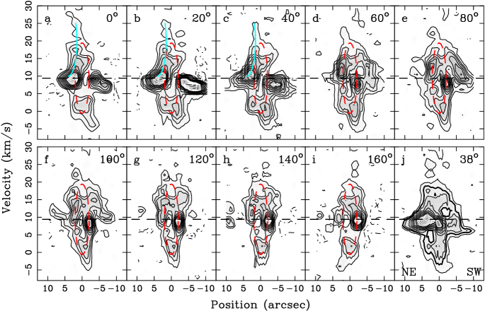
Figure 6: The position-velocity (PV) diagram cuts at the position of the O5 star (panel $a$ to $i$) at 9 different position angles, as indicated at the upper-right corner in each panel. Panel $j$ is the PV diagram along the white segments indicated in the lower panel of Fig. 5. To show the fainter emission at outer regions, the black contours are plotted in 2, 4, 6, 9, 12, 15, 18 and 21 $\times$ $\sigma$ and white contours in 24, 27, 30, 33, 36 $\times$ $\sigma$, where 1$\sigma=$0.16 Jy Beam^-1. The thick contour in panel $j$ represents the emission strength of 4$\sigma$. The dashed segments indicate the v_sys of 9.4 km s^-1. The red dashed ellipse marks the ring-like structure with a radius of 2$\arcsec$ and 10 km s^-1 and centered at the position of the O5 star and v_sys of 9.4 km s^-1. The majority of the gas is quiescent with a velocity close to $v_{sys}$. In panel $j$, a loop-like structure is seen at positions of $\pm$ 2$\arcsec$. A clump at a v_lsr of 0 km s^-1 is detected in all the PV cuts at different PA (panel $a$ to $i$). At PA of 0$\arcdeg$ to 40$\arcdeg$, the high velocity structure extending from the position of 2.5$\arcsec$ is clearly seen, as indicated by the blue arc.

The PV plots cut at various PAs at the position of the O5 star and cut along the extension in the NE and SW direction on the 2nd moment image (white segments on the lower panel of Fig. 5) are shown in Fig. 6. The strongest emission is at $v_{sys}$ with an extension of 18$\arcsec$, which suggests that the majority of the gas is quiescent. Besides the quiescent gas, a ring-like structure, indicated as red-dashed ellipses in Fig. 6, can be seen clearly, especially at the PA of 60$\arcdeg$ to 100$\arcdeg$. Both an infalling motion (e.g. Ho & Young 1996) and an expansion can produce a ring-like structure in the PV plots. In an infalling motion, the expected free-fall velocity is $\sim$ 5 km s^-1 for a central mass of 50 M_☉ at a distance of 2$\arcsec$ from the central star. This is smaller than the value measured in the ring-like structure in G5.89. This C¹⁷O 3-2 ring-like structure in the PV plots is therefore more likely tracing the expansion along with the HII region because of its high velocity ($\pm$10 km s^-1) and its dimension (2$\arcsec$ in radius). However, the ring structure is not complete. This may be because the material surrounding the HII region is not homogeneously distributed, or the HII region is not completely surrounded by the molecular gas.

Besides the expansion motion along with the HII region, there are higher velocity components extending up to 30 km s^-1 (red-shifted) and $-$5 km s^-1 (blue-shifted) (Fig. 6). The high velocity structure extending from the position of 2.5$\arcsec$ to the velocity of $\sim$30 km s^-1 is clearly seen in the PV cuts at PA of 0$\arcdeg$ to 40$\arcdeg$ (indicated as cyan arcs in Fig. 6). These high velocity components are probably due to the sweeping motion of the molecular outflows in G5.89, because there is no other likely energy source which can move the material to such a high velocity. From the PV plots at the position of the O5 star at various PAs and the PV plot cut along the sharp dust ridge, we conclude that the molecular cloud is most likely both expanding along with the HII region and being swept-up by the molecular outflows, all in addition to the bulk of the quiescent gas.

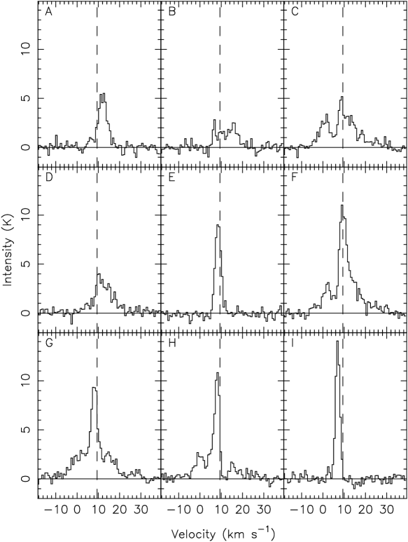
Figure 7: The spectra of the C¹⁷O 3-2 line at various positions as indicated in Fig. 5. The solid and dashed segments mark the intensity of 0 K and v_sys of 9.4 km s^-1, respectively. Note that the typical HII region expands at a velocity of $\pm$ 10 km s^-1. At position E and I, the spectra are narrowest.

The examination of the spectra at various positions also helps to analyze the kinematics in G5.89. The spectra (Fig. 7) near the HII ring (positions $C$, $D$, $F$, $G$ and $H$) have broad line-widths. Furthermore, the spectra are not Gaussian-like, or with distinct components at high velocities ($\pm$ 10 km s^-1). At position $F$ and $H$, both spectra show a strong peak at v_sys. The high velocity wing at the position $F$ is red-shifted, and it is blue-shifted at position H. This is consistent with the NS molecular outflow. The molecular gas near the positions $E$ and $I$ is more quiescent because of its narrow linewidth. The spectrum taken at position $I$ has a FWHM of 4 km s^-1 and a peak intensity at $\sim$ 7 km s^-1. Comparing with the spectra at other positions, the cloud around the position $I$ is relatively quiescent and unaffected by the HII region or the outflows. This cloud in the south near the position $I$ may be a more independent component which is further separated along the line of sight. We conclude that the C¹⁷O 3-2 spectra demonstrate that the kinematics and morphology have been strongly affected by the expansion of the HII region. The nearly circular structure in the PV plots, and in the channel maps near the systemic velocity, as well as the spectra, suggest that a significant part of the mass has been pushed by the HII region. An impact from the molecular outflow can also be seen in the PV plots and spectra.

5.3 Estimate of the B field strength

The B field strength projected in the plane of sky (B_⊥) can be estimated by means of the Chandrasekhar-Fermi (CF) method (Chandrasekhar & Fermi 1953; Falceta-Gonçalves, Lazarian, & Kowal 2008). In general, the CF method can be applied to both dust and line polarization measurements. We apply the CF method only to the dust continuum polarization, because there is no line polarization detected in this paper. Although the dust grains can also be mechanically aligned, the existing observational evidence in NGC 1333 IRAS4A (Girart et al. 2006) demonstrates that the dust grains can align with the B field in the low mass star formation regions. Here, we assume that the dust grains also align with the B field in G5.89.

The strength of B_⊥ can be calculated from:

$$B_{\bot}=Q\sqrt{4\pi\bar{\rho}}\frac{\delta v_{los,A}}{\delta\phi}=63\sqrt{n_{H_{2}}}\frac{\delta v_{los,A}}{\delta\phi}$$ (4)

Here, B_⊥ is in the unit of mG. The term Q is a dimensionless parameter smaller than 1. Q is $\sim$0.5 (Ostriker, Stone & Gammie 2001), depending on the inhomogeneities within the cloud, the anisotropies of the velocity perturbations, the observational resolution and the differential averaging along the line of sight. The term $\bar{\rho}$ is the mean density. $\delta\phi$ is the dispersion of the polarization angles in units of degree. $\delta v_{los,A}$ is the velocity dispersion along the line of sight in units of km s^-1, which is associated with the Alfvénic motion. $n_{H{2}}$ is the number density of H₂ molecules in units of 10⁷ cm^-3. It has been shown numerically that the CF method is a good approximation for $\delta\phi<25^{\arcdeg}$ (Ostriker, Stone, & Gammie (2001)).

$\delta v_{los,A}$ is estimated from $\delta v_{total}$ in the 2nd moment image (lower panel in Fig. 5). $\delta v_{total}$ contains the information of the dispersions caused by the Alfvénic turbulent motion ($\delta\textit{v}_{los,A}$) and the dispersions caused by the HII expansion and outflow motions ($\delta\textit{v}_{bulk}$). The relation of these three components is:

$$\delta v_{total}\sim\sqrt{\delta v_{los,A}^{2}+\delta v_{bulk}^{2}}$$

Here, we neglect the minor contributions from the thermal Doppler motions. The measured $\delta v_{total}$ at the positions of detected polarization are listed in Table 1. $\delta v_{total}$ is in the range of 1 to 6 km s^-1. However, the molecular gas near the HII region is clearly disturbed by both the HII expansion and the molecular outflows (see Sec. 4.3.1 and 5.2). Therefore, the detected $\delta v_{total}$ at these positions is dominated by the bulk motion. Since $\delta v_{total}$ in the relatively quiescent regions is more likely tracing the Alfvénic motion only, we adopt the minimum value $\delta v_{total}$ of 1 km s^-1 at these positions for $\delta v_{los,A}$ in order to derive B_⊥.

The term $n_{H_{2}}$ is $\sim$3$\times$10⁶ (cm^-3), estimated from the averaged $n_{H_{2}}$ from the 870$\mu$m dust continuum and the C¹⁷O 3-2 line emission (Sec. 4.1.2 and Sec. 4.3.2). $\delta\phi$ in Eq. 4 can be extracted from the observed standard deviation of the PAs $\delta\phi_{obs}$. $\delta\phi_{obs}$ contains both the observational uncertainty $\sigma_{\phi,obs}$ and $\delta\phi$. The relation is: $\delta\phi_{obs}^{2}$ = $\delta\phi^{2}+\sigma_{\phi,obs}^{2}$. Since the polarization in G5.89 results probably from two different systems (discussed in Sec. 4.2.1 and 4.2.2), it is more reasonable to separate these two groups when deriving $\delta\phi$. The derived $\sigma_{\phi,obs}$, $\delta\phi_{obs}$ and $\delta\phi$ are 3$\arcdeg$ and 11$\arcdeg$ and $\sim$11$\arcdeg$ for component ”o”, and 2$\arcdeg$, 18$\arcdeg$ and $\sim$18$\arcdeg$ for component ”x”, respectively. By using Eq. (4), the derived B_⊥ is 3mG and 2mG for component ”o” and ”x”, respectively.

The estimated B_⊥ is highly uncertain. Due to the bulk motions, it is difficult to extract the $\delta v_{los,A}$ component from the observed $\delta v_{total}$. The uncertainty introduced from $\delta v_{los,A}$ is within a factor of 6. Of course, the grouping of ”o” and ”x” components of the polarization, as motivated in Sec. 4.2.1, 4.2.2 and 5.2, is not a unique interpretation. If $\delta\phi$ is calculated without grouping, a more complex model of the larger scale B field morphology is needed to calculate the deviation due to the Alfvénic motion. More observations with sufficient uv coverage are required to establish such a model. Based on the standard deviation $\delta\phi$ of 39$\arcdeg$ from the detected polarization without subtracting the larger scale B field and without grouping, the calculated lower limit of B_⊥ is $\sim$1mG. Therefore, the estimated B_⊥ from the grouping of component ”o” and ”x” seems reasonable. The value is comparable to the ones estimated via the CF method in other massive star formation regions with an angular resolution of a few arcseconds: $\sim$ 1mG in DR 21(OH) (Lai et al. 2003) and $\sim$1.7 mG in G30.79 FIR 10 (Cortes & Crutcher 2006). Moreover, B_⊥ is similar to B_∥ measured from the Zeeman pairs of the OH masers by Stark et al. (2007), ranging from $-$2 to 2 mG. Although B_∥ measured from OH masers is most likely tracing special physical conditions, such as shocks or dense regions, it is the only direct measurement of B_∥ in G5.89, and hence, is of interest to compare. Assuming B_⊥ and B_∥ have the same strengths of 2mG, the total B field strength in G5.89 is $\sim$ 3 mG.

5.4 Collapsing cloud or not?

The mass to flux ratio $\lambda$, a crucial parameter for the magnetic support/ambipolar diffusion model, can be calculated from: $\lambda$ = 7.6 $\times$ 10^-21 $\frac{N_{H_{2}}}{B}$ (Mouschovias & Spitzer 1976; Nakano & Nakamura 1978). $N_{H_{2}}$ is in cm^-2. $B$ is in $\mu$G. In the case of $\lambda$ $<$ 1, the cloud is in a subcritical stage and magnetically supported. In the case of $\lambda$ $>$ 1, the cloud is in a collapsing stage.

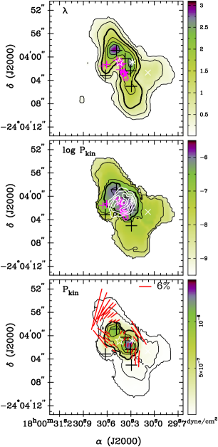
Figure 8: Upper panel: Image of the mass to flux ratio $\lambda$ in both contours and color scale. $\lambda$ is derived using the C¹⁷O 3-2 emission line assuming a uniform total B field strength of 3 mG, which corresponds to a B field pressure (P_B) of 3.6$\times$10^-7 dyne cm^-2. The thick black contour marks $\lambda$=1. The thin black contours mark $\lambda$=0.1, 0.5, 1.5, 2, 2.5. The strength of $\lambda$ in color scale is indicated in the wedge. The other symbols are the same as in Fig. 2. Middle panel: Image of the derived kinetic pressure (P_kin) in log scale in both black contours and color scale. The thick black contour marks $log$ $P_{kin}$ $=$ $-$6.45, which is equal to P_B=3.6$\times$10^-7 dyne cm^-2. The thin black contours mark $log$ P_kin = $-$6, $-$7, $-$8, and $-$9. The white contours represent the 2cm free-free emission starting from and stepping in 72 mJy Beam^-1. The wedge is in the units of $log$ dyne cm^-2. Lower panel: Image of P_kin in linear scale in both black contours and color scale. P_kin is in the unit of dyne cm^-2. The thick black contour marks P_kin $=$ 3.6$\times$10^-7 dyne cm^-2. The thin black contours mark P_kin = (0.3, 3, 60, 90, 120)$\times$10^-8. The red segments represent the 870 $\mu$m polarization above 3$\sigma_{I_{p}}$, detected in this paper.

Since there is no observation of the B field strength as a function of position in the entire cloud, we assume that the B field is uniform with the strength of 3 mG in the entire cloud when $\lambda$ is calculated. For consistency, when comparing with the kinetic pressure in the next section, $N_{H_{2}}$ is derived from the C¹⁷O 3-2 emission (section 4.3.2). The derived $\lambda$ in G5.89 is $>$1 in most parts of the molecular cloud, as shown in the upper panel of Fig. 8. If the statistical geometrical correction factor of $\frac{1}{3}$ is considered (Crutcher 2004), the $\lambda_{corr}$ in the sharp dust ridge is still close to 1, whereas at the positions of the component ”o” and the outer part, it is much smaller than 1. This suggests that G5.89 is probably in a supercritical phase near the HII region and in a subcritical phase in the outer part of the dust core.

This conclusion is based on the assumption that the B field in the entire cloud is uniform with a strength of 3 mG. This assumption seems to be crucial at first glance. However, the derived $\lambda$ increases from 0.1 to 2.5 toward the UCHII region, which is due to the high contrast of the column density across the cloud. Unless the actual B field strength differs by a factor of 25 across the region and compensates for the contrast in the column density, such a variation of $\lambda$ in G5.89 is indeed possible.

5.5 Compressed field?

The coincident location of the detected polarization of component ”x” and the sharp dust ridge is quite interesting. One possible scenario is that the B field lines are compressed by the shock front, i.e. HII expansion. In a magnetized large molecular cloud with a B field traced by a component ”o”, and with a shock sent out from the east of the narrow dust ridge, we expect a rapid change of the polarization PA. This is similar to the results in magnetohydrodynamic simulations by Krumholz et al. (2007). Because of our limited angular resolution, polarization with a large dispersion in the PAs over a small physical scale will be averaged out within the synthesized beam. In our result, in fact, there is a gap where polarized emission is not detected right next to the sharp dust ridge, and a series of OH masers are detected in this gap. Note that the OH masers are most likely from the shock front. From the discussion in Sec. 5.2, evidence for the molecular cloud expanding with the HII region is found in the molecular gas traced by the C¹⁷O 3-2 emission. The 870$\mu$m sharp dust ridge can be explained by the swept-up material along with the molecular gas from the HII expansion. In this scenario, the component ”o” is tracing the B field in the pre-shock region, while the ”x” component is tracing the compressed field.

However, the swept-up flux density (summation of the flux density of SMA-N, SMA-1 and SMA-2 reported in Hunter et al. 2008) is $\sim$ 20% of the total detected flux density in this paper. This requires a huge amount of energy to sweep up the material with this mass. Is the radiation pressure (P_rad) from the central star large enough to overcome the kinetic pressure (P_kin) and the B field pressure (P_B)? Here we compare these pressure terms.

P_rad can be calculated from the luminosity in G5.89 following the equation: P_rad $=$ $\frac{L}{cA}$, where $L$, $c$ and A are the luminosity, speed of light and the area, respectively. Since the G5.89 region is dense, most of the radiation is absorbed and redistributed into the surrounding material. The total far infrared luminosity of G5.89 is 3$\times$10⁵L_☉ (Emerson, Jennings, & Moorwood 1973) and the radius of the HII region at 2cm is $\sim$ 2$\arcsec$ (4000 AU). The energy density and hence, the radiation pressure (P_rad) in the sphere with a radius of 2$\arcsec$ is 8.5$\times$10^-7 (dyne cm^-2).

P_kin is calculated by using the 0th moment ($MOM0$) and 2nd moment ($MOM2$) images of the C¹⁷O 3-2 line:

$$P_{kin}=\frac{1}{2}\rho\delta v_{total}^{2}=3.4\times 10^{-9}\times(MOM0)\times(MOM2)^{2}$$ (5)

where P_kin is in dyne cm^-2, $\rho$ is the gas density in g cm^-3 and $\delta v_{total}$ is the velocity dispersion in cm s^-1, $MOM0$ is in units of K km s^-1, and $MOM2$ is in units of km s^-1. $\rho$ is calculated following Sec. 4.3.2, with the size of 0.13 pc for the molecular cloud along the line of sight. The derived P_kin image is shown in the middle and lower panels of Fig. 8. P_kin is in the range of $\sim$ 1$\times$10^-9 to 1.4$\times$10^-6 dyne cm^-2. P_kin is calculated under the assumption that the length along the line of sight is uniform in G5.89, which is the main bias in the calculation. The estimated total B field strength is 3 mG, thus the B-field pressure (P_B) is 3.6$\times$10^-7 (dyne cm^-2). Although the upper limit of P_kin is 1.6 times larger than P_rad at a radius of 2$\arcsec$, any variation of the structure in the direction along the line of sight in G5.89 - which is most likely the case - will affect the estimated P_kin. Nevertheless, P_rad is at the same order as P_kin and P_B at the radius of 2$\arcsec$ around the O5 star. Therefore, in terms of pressure, the radiation from the central star is likely sufficient to sweep up the material and compress the B field lines along the narrow dust ridge. $\lambda_{corr}$ close to 1 near the UCHII region suggests that the B fields play a minor role as compared with the gravity.

The B field direction traced by component ”x” is parallel to the major axis of this sharp dust ridge, which is also seen in some other star formation sites such as Cepheus A (Curran $\&$ Chrysostomou 2007) and DR 21(OH) (Lai et al. 2003). However, in most of the cases, the detected B field direction is parallel to the minor axis of the dust ridge, e.g. W51 e1/e2 cores (Lai et al. 2001) and G34.4+0.23 MM (Cortes et al. 2008), which agrees with the ambipolar diffusion model. A possible explanation is that the polarization is from the swept-up material, which interacts with the original dense filament. Thus, the polarization here may represent the swept-up field lines. This scenario is supported by the energy density and also the morphology of the field lines in the case of G5.89.

5.6 Comparison with Other Star Formation Sites

The detected B field structure in the G5.89 region is more complicated than the B fields in other massive star formation sites detected so far with interferometers. Both the compressed field structure and the more organized larger scale B field are detected in G5.89.

The B field lines vary smoothly in the cores at earlier star formation stages, such as the W51 e1/e2 cores (Lai et al. 2001), G34.4+0.23 MM (Cortes et al. 2008) and NGC 2024 FIR 5 (Lai et al. 2002). These cores are still in a collapsing stage (Ho et al. 1996 ; Ramesh et al. 1997; Mezger et al. 2001). Among these observations, the B fields inferred from the dust polarization show an organized structure over the scale of 10⁵ AU (15$\arcsec$) at a distance of 7 kpc in the W51 e1/e2 cores and also on the scale of 10⁵ AU (35$\arcsec$) at a distance of 3.9 kpc in G34.4+0.23 MM. In contrast, the B fields in NGC 2024 FIR 5, which is closer at a distance of 415 pc, show an hourglass morphology on a scale of 4$\times$10³ AU (9$\arcsec$). Such small scale structures would not be resolved in the current data of W51 e1/e2 core and G34.4+0.23 MM due to the resolution effect. Compared to these sources, G5.89 is more complicated with polarization structures on both small (4$\times$10³ AU) and large (2$\times$10⁴ AU) scales. However, higher angular resolution polarization images of the cores in the earlier stages are necessary in order to compare the B field morphology with the later stages in the massive star formation process. At this moment, we cannot conclude at which stage the B field structures become more complex.

Currently, the best observational evidence supporting the theoretical accretion model is the polarization observation of the source NGC 1333 IRAS 4A (Girart, Rao & Marrone 2006) carried out with the SMA. The NGC 1333 IRAS 4A is a low mass star formation site, at a distance of $\sim$300 pc. The detected pinched B-field structure is at a scale of 2400 AU (8$\arcsec$). If NGC 1333 IRAS 4A were at a distance of 2kpc, we could barely resolve it at our resolution of 3$\arcsec$. Higher angular resolution polarization measurements are required to resolve the underlying structure in G5.89.

6 Conclusions and Summary

High angular resolution (3$\arcsec$) studies at 870$\mu$m have been made of the magnetic (B) field structures, the dust continuum structures, and the kinematics of the molecular cloud around the Ultra-Compact HII region G5.89-0.39. The goal is to analyze the role of the B field in the massive star forming process. Here is the summary of our results:

1. The gas mass (M_gas) is estimated from the dust continuum and from the C¹⁷O 3$-$2 emission line. The continuum emission at 870 $\mu$m is detected with its total flux density of 12.6$\pm$1.3 Jy. After removing the free-free emission from the detected continuum, the flux density of the 870 $\mu$m dust continuum is 7.7 Jy, which corresponds to M_gas $\sim$300 M_☉. M_gas derived from the detected C¹⁷O 3-2 emission line is $\sim$100 M_☉, which is 3 times smaller than the value derived from the dust continuum. The discrepancy of M_gas derived from the dust continuum and the C¹⁷O emission line is also seen in other UCHII regions, e.g. Hofner et al. (2000). The lower values measured from C¹⁷O could be due to optical depth effects or abundance problems.

2. The linearly polarized 870 $\mu$m dust continuum emission is detected and resolved. The dust polarization is not uniformly distributed in the entire dust core. Most of the polarized emission is located around the HII ring, and there is no polarization detected in the southern half of the dust core except at the very southern edges. The position angles (PAs) of the polarization vary enormously but smoothly in a region of 2$\times$10⁴ AU (10$\arcsec$), ranging from $-$60$\arcdeg$ to 61$\arcdeg$. Furthermore, the polarized emission is from organized patches, and the distribution of the PAs can be separated into two groups. We suggest that the polarization in G5.89 traces two different components. The polarization group ”x”, with its PAs ranging from $-$60$\arcdeg$ to $-$4$\arcdeg$, is located at the 870$\mu$m sharp dust ridge. In contrast, the group ”o”, with its PAs ranging from 33$\arcdeg$ to 61$\arcdeg$, is at the periphery of the sharp dust ridge. The inferred B field direction from group ”x” is parallel to the major axis of the 870$\mu$m dust ridge. One possible interpretation of the polarization in group ”x” is that it may represent swept-up B field lines, while the group ”o” traces more extended structures. In the G5.89 region, both the large scale B field (group ”o”) and the compressed B field (group ”x”) are detected.

3. By using the Chandrasekhar-Fermi method, the estimated strength of B_⊥ from component ”o” and from component ”x” is in between 2 to 3 mG, which is comparable to the Zeeman splitting measurements of B_∥ from the OH masers, ranging from $-$2 to 2 mG by Stark et al. (2007). The derived lower limit of B_⊥ from the detected polarization without grouping and without modeling larger scale B field is $\sim$1mG. Assuming that B_⊥ and B_∥ have the same strengths of 2 mG in the entire cloud, the derived $\lambda$ increases from 0.1 to 2.5 toward the UCHII region, which is due to the high contrast of the column density across the cloud. Unless the actual B field strength differs by a factor of 25 across the region and compensates for the contrast in the column density, such a variation of $\lambda$ in G5.89 is suggested. The corrected mass to flux ratio ($\lambda_{corr}$) is closer to 1 near the HII region and is much smaller than 1 in the outer parts of the dust core. G5.89 is therefore most likely in a supercritical phase near the HII region.

4. The kinematics of the molecular gas is analyzed using the C¹⁷O 3-2 emission line. From the analysis of the channel maps, the position velocity plots and spectra, the molecular gas in the G5.89 region is expanding along with the HII region, and it is also possibly swept-up by the molecular outflows. Assuming the size along the line of sight is uniform in G5.89, P_kin is in the range of $\sim$ 1$\times$10^-9 to 1.4$\times$10^-6 dyne cm^-2. The calculated radiation pressure (P_rad) at a radius of 2$\arcsec$ and the B field pressure (P_B) with a field strength of 3mG are 8.5$\times$10^-7 and 3.6$\times$10^-7 dyne cm^-2, respectively. Although the upper limit of P_kin is 1.6 times larger than P_rad at a radius of 2$\arcsec$, any variation of the structure in the direction along the line of sight in G5.89 - which is most likely the case - will affect the estimated P_kin. Nevertheless, P_rad is on the same order as P_kin and P_B at the radius of 2$\arcsec$ around the O5 star. The scenario that the matter and B field in the 870$\mu$m sharp dust ridge have been swept-up is supported in terms of the available pressure.

G5.89 is in a more evolved stage as compared with the corresponding structures of other sources in the collapsing phase. The morphologies of the B field in the earlier stages of the evolution show systematic or smoothly varying structures, e.g. on the scale of 10⁵ AU for W51 e1/e2 and G34.4+0.23 MM, and on the scale of 4$\times$10³ AU for NGC 2024 FIR 5. With the high resolution and high sensitivity SMA data, we find that the B field morphology in G5.89 is more complicated, being clearly disturbed by the expansion of the HII region and the molecular outflows. The large scale B field structure on the scale of 2$\times$10⁴ AU in G5.89 can still be traced with dust polarization. From the analysis of the C¹⁷O 3-2 kinematics and the comparison of the available energy density (pressure), we propose that the B fields have been swept up and compressed. Hence, the role of the B field evolves with the formation of the massive star. The ensuing luminosity, pressure and outflows overwhelm the existing B field structure.

Table 1: SMA dust polarization at 870 $\mu m$

$\triangle$x	$\triangle$y	Ip	%	PA	$\delta v_{total}$	group
5.4	5	24	21.5 $\pm$ 4.6	-14 $\pm$ 6	1.0	x
4.8	5	26	18.3 $\pm$ 3.6	-22 $\pm$ 5	1.2	x
4.2	5	23	11.9 $\pm$ 2.6	-33 $\pm$ 6	1.2	x
3.6	5	20	9.1 $\pm$ 2.3	-43 $\pm$ 7	1.2	x
3	5	16	7.7 $\pm$ 2.5	-46 $\pm$ 9	1.2	x
4.8	4	18	9.3 $\pm$ 2.6	-22 $\pm$ 8	1.0	x
4.2	4	21	7 $\pm$ 1.7	-31 $\pm$ 7	1.5	x
3.6	4	21	4.6 $\pm$ 1.1	-41 $\pm$ 7	1.5	x
3	4	19	3.7 $\pm$ 1	-49 $\pm$ 8	1.5	x
2.4	4	14	3.7 $\pm$ 1.3	-53 $\pm$ 10	1.4	x
3	3	16	1.9 $\pm$ 0.6	-54 $\pm$ 9	2.5	x
2.4	3	17	2.1 $\pm$ 0.6	-59 $\pm$ 8	2.2	x
1.8	3	15	2.3 $\pm$ 0.8	-60 $\pm$ 10	2.0	x
4.2	1	16	7.6 $\pm$ 2.4	53 $\pm$ 9	3.4	o
3.6	1	16	2.8 $\pm$ 0.9	60 $\pm$ 9	4.3	o
1.2	1	17	1.4 $\pm$ 0.4	-29 $\pm$ 8	4.0	x
0.6	1	17	1.6 $\pm$ 0.5	-29 $\pm$ 8	3.3	x
-1.2	1	17	6.7 $\pm$ 2	38 $\pm$ 9	3.8	o
-1.8	1	16	14.2 $\pm$ 4.5	33 $\pm$ 9	1.8	o
4.8	0	15	11.2 $\pm$ 3.6	38 $\pm$ 9	2.7	o
4.2	0	16	6 $\pm$ 1.9	48 $\pm$ 9	3.6	o
3.6	0	16	3 $\pm$ 1	56 $\pm$ 9	4.0	o
0.6	0	22	1.5 $\pm$ 0.3	-24 $\pm$ 7	4.6	x
0	0	17	1.3 $\pm$ 0.4	-18 $\pm$ 9	4.5	x
-1.2	0	15	2.9 $\pm$ 1	39 $\pm$ 10	3.9	o
3	-1	14	1.6 $\pm$ 0.6	58 $\pm$ 10	4.5	o
2.4	-1	15	1.4 $\pm$ 0.5	61 $\pm$ 9	5.8	o
0.6	-1	18	1.2 $\pm$ 0.3	-16 $\pm$ 8	5.3	x
0	-1	22	1.5 $\pm$ 0.3	-15 $\pm$ 6	5.0	x
-0.6	-1	17	1.5 $\pm$ 0.4	-12 $\pm$ 8	4.8	x
2.4	-2	15	1.8 $\pm$ 0.6	59 $\pm$ 9	5.9	o
0	-2	18	1.4 $\pm$ 0.4	-10 $\pm$ 8	5.0	x
-0.6	-2	23	2.2 $\pm$ 0.5	-14 $\pm$ 6	4.8	x
-1.2	-2	19	2.8 $\pm$ 0.8	-16 $\pm$ 8	4.7	x
-0.6	-3	18	1.8 $\pm$ 0.5	-4 $\pm$ 8	3.3	x
-1.2	-3	22	3.6 $\pm$ 0.8	-8 $\pm$ 6	2.4	x
-1.8	-3	19	6 $\pm$ 1.6	-6 $\pm$ 8	2.7	x
-1.2	-4	16	2.3 $\pm$ 0.7	4 $\pm$ 9	1.4	x
-1.8	-4	17	4.6 $\pm$ 1.3	-3 $\pm$ 8	1.4	x

Note. — $\triangle$x & $\triangle$y: offsets in arcsecond from the coordinate (J2000): $\alpha=18:00:30.32$, $\delta=-24:04:00.48$. $I_{p}$: the polarized intensity in mJy Beam^-1. %: polarization percentage, defined as the ratio of I_p/I. PA: position angle from the north to the east in degree. $\delta v_{total}$: total dispersion velocity (2nd moment) measured in the C¹⁷O 3-2 emission line in km s^-1. All data listed are above 3$\sigma_{I_{p}}$.

References

- (1) Acord, J. M., Churchwell, E., & Wood, D. O. S. 1998, ApJ, 495, 107
- (2) Cesaroni, R., Walmsley, C. M., Koempe, C., & Churchwell, E. 1991, A&A, 252, 278
- (3) Chandrasekhar, S., & Fermi, E. 1953, ApJ, 118, 113
- (4) Choi, M., Evans II, N., & Jaffe, D. T. 1993, ApJ, 417, 624
- (5) Churchwell 1997, ApJ, 479, L59
- (6) Cortes, P. C., Crutcher, R. M., & Watson, W. D. 2005, 628, 780
- (7) Cortes, P., & Crutcher, R. M. 2006, ApJ, 639, 965
- (8) Cortes, P., Crutcher, R. M., & Matthews, B. 2006, ApJ, 650, 246
- (9) Cortes, P., Crutcher, R. M., Shepherd, D. S., & Bronfman, L. 2008, ApJ, 676, 464
- (10) Crutcher, R. M. 2004, ApSS, 292, 225
- (11) Curran, R. L. & Chrysostomou, A. 2007, MNRAS, 382, 699
- (12) Deguchi, S. & Watson, W. 1984, ApJ, 285, 126
- (13) Draine, & Weingartner 1996, ApJ, 470, 551
- (14) Elmegreen, B. G., & Scalo, J. 2004, ARA&A, 42, 211
- (15) Emerson, J. P., Jennings, R. E., & Moorwood, A. F. M. 1973, ApJ, 184, 401
- (16) Falceta-Gonçalves, D., Lazarian, A., & Kowal, G. 2008, ApJ, 679, 537
- (17) Feldt, M., Stecklum, B., Henning, Th., Launhardt, R., & Hayward, T. L. 1999, A&A, 346, 243
- (18) Feldt, M., Puga, E., Lenzen, R., Henning, Th., Brandner, W., Stecklum, B., Lagrange, A.-M., Gendron, E., & Rousset, G. 2003, ApJ, 599, L91
- (19) Fiedler, R. A., & Mouschovias, T. Ch. 1993, ApJ, 415, 680
- (20) Fish, V. L, Reid, M. J., Argon, A. L., & Zheng, X.-W. 2005, ApJS, 160, 220
- (21) Frerking, M. A., & Langer, D. L., & Wilson, W. W. 1982, ApJ, 262, 590
- (22) Galli, D., & Shu, F. H. 1993, ApJ, 417, 243
- (23) Girart, J. M., Crutcher, R. M. & Rao, R. 1999, ApJ, 525, L109
- (24) Girart, J. M., Rao, R., & Marrone, D. P. 2006, Sci, 313, 812
- (25) Goldreich, P., & Kylafis, N. D. 1981, ApJ, 243, 75
- (26) Gonçalves, J., Galli, D., & Walmsley, M. 2005, A&A, 430, 979
- (27) Harvey, P. M., & Forveille, T. 1988, A&A, 197, L19
- (28) Ho, P. T. P., Moran, J. M., & Lo, K. Y. 2004, ApJ, 616, 1
- (29) Ho, P. T. P., & Young, L. M. 1996, ApJ, 472, 742
- (30) Hofner, P., & Churchwell 1996, A&AS, 120, 283
- (31) Hofner, P., Wyrowski, F., Walmsley, C. M., & Churchwell, E. 2000, ApJ, 536, 393
- (32) Hunter, T. R., Churchwell, E., Watson, C., Cox, P., Benford, D. J., & Roelfsema, P. R. 2000, AJ, 119, 2711
- (33) Hunter, T. R., Brogan, C. L., Indebetouw, R., & Cyganowski, C. J. 2008, 680, 127
- (34) Kramer, C., Alves, J., Lada, C., Lada, E., Sievers, A., Ungerechts, H., & Walmsley, M. 1999, A&A, 342, 257
- (35) Krumholz, M., Stone, J. M., & Gardiner, T. A. 2007, ApJ, 671, 518
- (36) Kurtz, S., Hofner, P., & Alvarez, C. V. 2004, ApJS, 155, 149
- (37) Kylafis, N. D. 1983, ApJ, 267, 137
- (38) Lai, S.-P., Crutcher, R. M., Girart, J. M., & Rao, R. 2001, ApJ, 561, 864
- (39) Lai, S.-P., Crutcher, R. M., Girart, J. M., & Rao, R. 2002, ApJ, 566, 925
- (40) Lai, S.-P., Girart, J. M., & Crutcher, R. M. 2003, ApJ, 598, 392
- (41) Lazarian, A. 2007, Journal of Quantitative Spectroscopy & Radiative Transfer, 106, 255
- (42) Lazarian, A. & Hoang, T. 2007, MNRAS, 378, 910
- (43) Lis, D. C., Serabyn, E., Keene, Jocelyn, Dowell, C. D., Benford, D. J., Phillips, T. G., Hunter, T. R., Wang, N. 1998, 509, 299 Mac Low
- (44) Mac Low, M.-M., & Klessen, R. S. 2004, Rev. Mod. Phys., 76, 125
- (45) Marrone, D. & Rao, R. 2008, arXiv:0807.2255
- mezger (1992) Mezger, P. G., Sievers, A. W., Haslam, C. G. T., Kreysa, E., Lemke, R., Mauersberger, R., & Wilson, T. L. 1992, A&A, 256, 631
- (47) Mouschovias, T. Ch. 1976, ApJ, 207, 141
- (48) Mouschovias, T. Ch., & Spitzer, L. 1976, ApJ, 210, 326
- (49) Mouschovias, T. Ch. & Ciolek, G. E. 1999, in The Origin of Stars and Planetary Systems, ed. C. J. Lada & N. D. Kylafis (Kluwer: Dordrecht), p. 305
- (50) Nakano, T., & Nakamura, T. 1978, PASJ, 30, 681
- ostriker (2001) Ostriker, E. C., Stone, J. M., & Gammie, C. F. 2001, ApJ, 546, 980
- (52) Puga, E., Feldt, M., Alvarez, C., Henning, Th., Apai, D., Coarer, E. Le, Chalabaev, A., & Stecklum, B. 2006, ApJ, 641, 373
- (53) Ramesh, B., Bronfman, L., & Deguchi, S. 1997, PASJ, 49, 307
- (54) Rao, R., Crutcher, R. M., Plambeck, R. L., & Wright, M. C. H. 1998, ApJ, 502, L75
- (55) Rohlfs, K., & Wilson, T. L. 2004, Tools of Raido Astronomy (4th ed; Berlin: Springer)
- (56) Sault, R. J., Teuben, P. J., & Wright, M. C. H. 1995, in ASP Conf. Ser. 77, Astronomical Data Analysis Software and Systems IV, ed. R. A. Shaw, H. E. Payne, & J. J. E. Hayes (San Francisco: ASP), 433
- (57) Sault, R. J., Hamaker, J. P., & Bregman, J. D. 1996, A&AS, 117, 149
- (58) Shu, F., Allen, A., Shang, H., Ostriker, E. C., & Li, Z.-Y. 1999, in The Origin of Stars and Planetary Systems, ed. Charles J. Lada & Nikolaos D. Kylafis, (Kluwer: Dordrecht), p. 193
- Sollins (2004) Sollins, P. K., Hunter, T. R., Battat, J., Beuther, H., Ho, P. T. P., Lim, J., Liu, S. Y., Ohashi, N., Sridharan, T. K., Su, Y. N., Zhao, J.-H., & Zhang, Q. 2004, ApJ, 616, 35
- (60) Stark, D. P., Goss, W. M., Churchwell, E. Fish, V. L., & Hoffman, I. M. 2007, ApJ, 656, 943
- (61) Watson, C., Churchwell, E., Zweibel, E. G., & Crutcher, R. M. 2007, ApJ, 657, 318
- (62) Wood, D. O. S., & Churchwell, E. 1989, ApJS, 69, 831
- (63) Zijlstra, A. A., Pottasch, S. R., Engels, D., Roelfsema, P. R., Hekkert, P. T., & Umana, G. 1990, MNRAS, 246, 217