Global Attractivity of the Equilibrium
of a Difference Equation:
An Elementary Proof Assisted by Computer Algebra System

Abstract

Let $p$ and $q$ be arbitrary positive numbers. It is shown that if $q<p$, then all solutions to the difference equation

$$x_{n+1}=\frac{p+q\,x_{n}}{1+x_{n-1}},\quad n=0,1,2,\ldots,\quad x_{-1}>0,\ x_{0}>0$$ (E)

converge to the positive equilibrium $\overline{x}=\frac{1}{2}\left(q-1+\sqrt{(q-1)^{2}+4\,p}\right)$.

The above result, taken together with the 1993 result of Kocić and Ladas for equation (E) with $q\geq p$, gives global attractivity of the positive equilibrium of (E) for all positive values of the parameters, thus completing the proof of a conjecture of Ladas.

Key Words: difference equation, rational, second order, global attractivity, equilibrium
AMS 2000 Mathematics Subject Classification: 39A11

1 Introduction and Statement of Main Theorem

The difference equation

$$x_{n+1}=\frac{p+q\,x_{n}}{1+x_{n-1}},\quad n=0,1,2,\ldots,\quad x_{-1}>0,\ x_{0}>0$$ (E)

has a unique equilibrium $\overline{x}=\frac{1}{2}\left(q-1+\sqrt{(q-1)^{2}+4\,p}\right)$. In 1993, V. Kocić and G. Ladas proved in [4] (namely, part (e) of Theorem 3.4.3) that for $q\geq p>0$, all solutions to Eqn.(E) converge to the equilibrium. Since then the region of positive parameters $p,\ q$ for which global attractivity of the equilibrium holds has been extended in several publications: V. Kocic, G. Ladas, and I. W. Rodrigues [5], C. H. Ou, H. S. Tang and W. Luo [14], H. A. El-Morshedy [2], R. Nussbaum [15], V. Jiménez López [3]. However, there is a large region of parameters that is not covered by the results obtained in those publications (see Figure 1). Indeed, a well known conjecture of Ladas states the positive equilibrium to (E) is a global attractor for all positive values of the parameters $p$ and $q$, (for example, see [11], [7], [8]). The authors in reference [12] claim to have proved the conjecture, but there is a mistake in their proof, see [3] for details on this.

The main result of this work, given below, establishes global attractivity of the equilibrium of (E) for $q<p$, thus completing the proof of the conjecture.

Main Theorem If $0<q<p$, then all solutions to the difference equation (E) converge to the positive equilibrium $\overline{x}$.

Figure 1: Boundaries of regions in parameter space. Key: (a) $q\geq p$ (Kocić-Ladas, 1993), (b) $2(q+1)\geq p$ (Kocić-Ladas-Rodrigues, 1993), (c) $2(q^{3}-q^{2}+q+\sqrt{q^{4}-1}-1)/(q-1)^{2}\geq p$ (Ou-Tang-Luo, 2000), (d) $\frac{1}{2}\left(q+\sqrt{(q-1)^{2}+4p}-1\right)\leq\frac{q^{2}+1}{q-1}$ (El-Morshedy, 2003, and Nussbaum, 2007) (e) $4\,p\,(q-1)^{2}\geq 25$ Jiménez López (2008). It is interesting to note that Nussbaum obtained El-Morshedy’s bound expressed in different form. Also, Jiménez López’ region is an improvement on regions obtained previously by Ou-Tang-Luo, El-Morshedy, and Nussbaum for $q$ near $1$ and $p\geq 112.1$ (not shown in the figure). The point $(p,q)=(20,4)$ is in the exterior of all regions bounded by the different curves.

The study of Eq.(E) is facilitated by the introduction of a suitable change of variables, and thus we begin with it. The substitutions

$$p\,=\,\frac{\alpha}{A^{2}},\quad q\,=\,\frac{1}{A},\quad\mbox{ and }\quad\ x_{\ell}\,=\,q\,y_{\ell}\ (\,\ell=-1,0,2,\ldots\,)$$ (1)

in Eq.(E) yield the equation

$$y_{n+1}=\frac{\alpha+y_{n}}{A+y_{n-1}},\quad n=0,1,2,\ldots,\quad y_{-1},\,y_{0}\in(0,\infty)$$ (2)

The equilibria $\overline{x}$ of Eq.(E) and $\overline{y}$ of Eq.(2) satisfy

$$\overline{x}=q\,\overline{y}$$ (3)

One may view Lyness’ equation (see [10]),

$$z_{n+1}=\frac{\tilde{\alpha}+z_{n}}{z_{n-1}},\quad n=0,1,2,\ldots,\quad z_{-1},\,z_{0}\in(0,\infty)$$ (4)

as a limit case of (2) that results by setting $A=0$. Lyness’ equation is known to posess an invariant function [9] i.e., a continuous, nonconstant real valued function $g(x,y)$ defined on $(0,\infty)\times(0,\infty)$ such that every solution $\{z_{n}\}$ to (4) satisfies

$$g(z_{n+1},z_{n})=g(z_{0},z_{-1}),\quad n=0,1,2,\ldots$$ (5)

A formula for $g(x,y)$ was found by Lyness [13] for $\tilde{\alpha}=1$, and for positive $\tilde{\alpha}$ by Ladas [10]:

$$g(x,y)=\frac{(1+x)(1+y)(\tilde{\alpha}+x+y)}{x\,y}$$ (6)

It is easy matter to show that $g(x,y)$ has a unique critical point on the positive quadrant, namely $(\overline{z},\overline{z})$, where $\overline{z}$ is the equilibrium of Eq.(4). Since $g(x,y)$ is large near the boundary of the positive quadrant, $g(x,y)$ has a strict global minimum which is is attained at $(\overline{z},\overline{z})$ (see [17], [6]), i.e.,

$$g(\overline{z},\overline{z})<g(x,y)\quad\mbox{for}\quad(x,y)\in(0,\infty)\times(0,\infty),\quad(x,y)\neq(\overline{z},\overline{z}).$$ (7)

The function $g(x,y)$ plays a fundamental role in our proof. See Figure 2.

                      

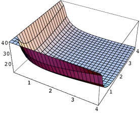
Figure 2: 3D-Plot and contour plot of the invariant function $g(x,y)$ for $\tilde{\alpha}=2$.

In Section 2 we prove several lemmas before giving the proof of the main theorem, which is done in order to simplify the exposition. For practical reasons, some of the calculations were performed with the computer algebra system (or CAS) Mathematica [16]. Code for such calculations, written in the Mathematica language, is given in Section 4.

2 Proofs

For typographical convenience we will use the symbol $u$ to represent the equilibrium $\overline{y}$ of Eq.(2). By direct substitution of the equilibrium $u=\overline{y}$ into (2) we obtain

$$\alpha=u^{2}+(A-1)\,u$$ (8)

By (8), $\alpha>0$ implies $u>1-A$. Using (8) to eliminate $\alpha$ from (2) gives the following equation, equivalent to (E):

$$y_{n+1}=\frac{u^{2}+(A-1)\,u+y_{n}}{A+y_{n-1}},\quad n=0,1,2,\ldots,\quad y_{-1},\,y_{0}\in(0,\infty)$$ (9)

Therefore, to prove the main theorem it suffices to prove that all solutions of Eq.(9) converge to the equilibrium $u$, and this is what the rest of the proof is geared to do.

The following statement is crucial for the proof of the main theorem.

Lemma 1

$u>1$ if and only if $q<p$.

Proof. Since $\overline{x}=q\,\overline{y}=q\,u$, we have $u>1$ if and only if $\overline{x}>q$, which holds if and only if $\frac{1}{2}\left(q-1+\sqrt{(q-1)^{2}+4\,p}\right)>q$. After an elementary simplification, the latter inequality can be rewritten as $q<p$. $\Box$

The hypothesis of the main theorem states $q<p$. In view of Lemma 1 we assume in the rest of the exposition that

$$u\ >\ 1$$ (10)

For the equilibrium $u$ of Eq.(9) to be also the the positive equilibrium of Lyness’ equation (4) one must have

$$u=\frac{\tilde{\alpha}+u}{u}$$ (11)

that is,

$$\tilde{\alpha}=u^{2}-u$$ (12)

For the value of $\tilde{\alpha}$ found in (12) the invariant function (6) becomes

$$g(x,y)=\frac{(1+x)(1+y)(u^{2}-u+x+y)}{x\,y}$$ (13)

One would hope that $g(x,y)$ turns out to be a Lyapunov function for Eq.(9) (see [6]). We shall see in the proof of Lemma 2 that this is not the case. Nevertheless we will be able to use the function $g(x,y)$ to complete the proof of the main theorem. First we need some elementary properties of the sublevel sets

$$S(c):=\{(s,t):g(s,t)\leq c\}\,,\quad c>0$$

We denote with $Q_{\ell}(u,u)$, $\ell=1,2,3,4$ the four regions

$$\begin{array}[]{rcl}Q_{1}(u,u)&:=&\{(x,y)\in(0,\infty)\times(0,\infty)\,:\ u\leq x,\ u\leq y\ \}\\ \\ Q_{2}(u,u)&:=&\{(x,y)\in(0,\infty)\times(0,\infty)\,:\ x\leq u,\ u\leq y\ \}\\ \\ Q_{3}(u,u)&:=&\{(x,y)\in(0,\infty)\times(0,\infty)\,:\ x\leq u,\ y\leq u\ \}\\ \\ Q_{4}(u,u)&:=&\{(x,y)\in(0,\infty)\times(0,\infty)\,:\ u\leq x,\ y\leq u\ \}\\ \\ \end{array}$$

Let

$$T(x,y):=\left(\,y\,,\,\frac{u^{2}+(A-1)u+y}{A+x}\,\right),\quad(x,y)\in(0,\infty)\times(0,\infty)$$ (14)

be the map associated to Eq. (9) (see [9]).

Lemma 2

If $(x,y)\in Q_{2}(u,u)\cup Q_{4}(u,u)\setminus\{(u,u)\}$, then $g(T(x,y))<g(x,y)$.

Proof. Set

$$\Delta_{1}(x,y):=g(x,y)-g(T(x,y))$$ (15)

A calculation yields

$$\Delta_{1}(x,y)=\frac{A\,\left(u-u^{2}+u\,x-y\right)\,\left(u-A\,u-u^{2}+A\,x+x^{2}-y\right)\,\left(1+y\right)}{x\,\left(A+x\right)\,y\,\left(-u+A\,u+u^{2}+y\right)}$$ (16)

By inspecting the factors in (16) one can see that $\Delta_{1}(x,y)$ changes sign on the line $y=u-u^{2}+u\,x$ and on the parabola $y=u-A\,u-u^{2}+A\,x+x^{2}$. Both curves are the graphs of strictly increasing functions of $x$ that intersect in the positive quadrant $\{(x,y):x>0,\ y>0\}$ at a unique point, namely $(u,u)$. At the point $(u,u)$, the slope of the parabola, $2\,u+A$, is larger than the slope of the line, $u$. See Figure 3. Clearly $\Delta_{1}(x,y)$ becomes negative for points $(x,y)$ between both curves, which, except for $(u,u)$, are contained in the complement of $Q_{2}(u,u)\cup Q_{4}(u,u)$.

Figure 3: $\Delta_{1}(x,y)<0$ for $(x,y)$ in the interior of the shaded region bounded by the line $y=u-u^{2}+u\,x$ and the parabola $y=u-A\,u-u^{2}+A\,x+x^{2}$.

$\Box$

Lemma 3

If $(x,y)\in Q_{1}(u,u)\cup Q_{3}(u,u)\setminus\{(u,u)\}$, then $g(T^{2}(x,y))<g(x,y)$.

Proof. Set

$$\Delta_{2}(x,y):=g(x,y)-g(T^{2}(x,y))$$ (17)

A calculation yields

$$\Delta_{2}(x,y)=\frac{-A^{2}\,u^{3}+A^{3}\,u^{3}+A^{4}\,u^{3}-A^{5}\,u^{3}+\cdots\mbox{\it 386 monomials}\cdots+2\,A^{2}\,u\,x^{2}\,y^{4}+A\,u\,x^{3}\,y^{4}+A\,y^{5}}{x\,\left(A+x\right)\,y\,\left(A+y\right)\,\left(-u+A\,u+u^{2}+y\right)\,\left(-u+A^{2}\,u+u^{2}+A\,u^{2}-u\,x+A\,u\,x+u^{2}\,x+y\right)}$$ (18)

Since $u^{2}-u>0$ by (10), the denominator of $\Delta_{2}(x,y)$ is positive. We now proceed to prove that the numerator of $\Delta_{2}(x,y)$, denoted by $Num$, is positive on $Q_{1}(u,u)\setminus\{(u,u)\}$. Begin by changing variables: $x=x_{0}+u$, $y=y_{0}+u$, where $x_{0}\geq 0$, $y_{0}\geq 0$ to get

$$Num=A\,u^{4}\,{x_{0}}^{2}+A\,u^{5}\,x_{0}^{2}+2\,A\,u^{6}\,x_{0}^{2}+2\,A\,u^{7}\,x_{0}^{2}+2\,A\,u^{3}\,x_{0}^{3}-A\,u^{4}\,x_{0}^{3}+\cdots\mbox{287 monomials}$$ (19)

Since some monomials in the right-hand-side of (19) have negative coefficient, it is not obvious that $Num>0$ for $x_{0}\geq 0$, $y_{0}\geq 0$, $(x_{0},y_{0})\neq(0,0)$. The last step here consists in considering subcases ($y_{0}>x_{0}$, $y_{0}<x_{0}$, and $y_{0}=x_{0}$). Substituting $y_{0}=x_{0}+k$ and $u=1+t$ for $k\geq 0$ and $t>0$, we obtain

$$Num=2\,A\,k^{2}+8\,A^{2}\,k^{2}+\cdots\mbox{368 monomials}\cdots+2\,A\,t\,x_{0}^{7}$$ (20)

By using a computer algebra system one can show that the coefficients of the monomials that form the expression in the right-hand-side of (20) are all positive integers. Thus $Num>0$ whenever (a) $x_{0}>0$, $y_{0}\geq x_{0}$. It can be easily verified that $Num>0$ in the other cases: (b) $y_{0}>0$, $y_{0}\leq x_{0}$, (c) $x_{0}=0$, $y_{0}>0$, and (d) $x_{0}>0$, $y_{0}=0$. We conclude that $\Delta_{2}(x,y)>0$ on $Q_{1}(u,u)\setminus\{(u,u)\}$. See Section 4 for details.

To verify that $Num>0$ on $Q_{3}(u,u)\setminus\{(u,u)\}$, we consider first $Num$ on the interior of $Q_{3}(u,u)$, and introduce the algebraic transformation

$$x=\frac{u\,w}{w+1},\quad y=\frac{u\,v}{v+1},\quad(w,v)\in(0,\infty)\times(0,\infty)$$

that maps the open positive quadrant $\{(w,v):w>0,\ v>0\}$ one-to-one and onto the interior of $Q_{3}(u,u)$. Then substitute $u=1+t$ with $t>0$, and consider subcases above, below, and on the diagonal just as we did before to conclude by direct inspection of coefficients that the transformed expression for $Num$ is positive.

A similar strategy works for proving $\Delta_{2}(x,y)>0$ on the open line segment with endpoints $(u,0)$ and $(u,u)$, and on the open line segment with endpoints $(0,u)$ and $(u,u)$. See Section 4 for details. $\Box$

Proof of the Main Theorem. Let $(\phi,\psi)\in(0,\infty)\times(0,\infty)$. Let $\{y_{n}\}_{n\geq-1}$ be the solution to (9) with initial condition $(y_{-1},y_{0})=(\phi,\psi)$, and let $\{T^{n}(\phi,\psi)\}_{n\geq 0}$ be the corresponding orbit of $T$. Define

$$\hat{c}:=\liminf_{n}g(T^{n}(\phi,\psi))$$ (21)

Note that $\hat{c}<\infty$, which can be shown by applying Lemma 2 and Lemma 3 repeatedly as needed to obtain a nonincreasing subsequence of $\{g(T^{n}(\phi,\psi))\}_{n\geq 0}$ that is bounded below by $0$. Let $\{g(T^{n_{k}}(\phi,\psi))\}_{k\geq 0}$ be a subsequence convergent to $\hat{c}$. Therefore there exists $c>0$ such that

$$g(T^{n_{k}}(\phi,\psi))\leq c\quad\mbox{ for all $k\geq 0$,}$$

that is,

$$T^{n_{k}}(\phi,\psi))\in S(c):=\{(s,t):g(s,t)\leq c\}\quad\mbox{for }k\geq 0$$

The set $S(c)$ is closed by continuity of $g(x,y)$. Boundedness of $S(c)$ follows from

$$0<x,\,y<\frac{(1+x)(1+y)(u^{2}-u+x+y)}{x\,y}=g(x,y)=c,\quad\mbox{for}\quad(x,y)\in S(c)$$

Thus $S(c)$ is compact, and there exists a convergent subsequence $\{T^{n_{k_{\ell}}}(\phi,\psi))\}_{\ell}$ with limit $(\hat{x},\hat{y})$ (say). Note that

$$\hat{c}=\lim_{\ell\rightarrow\infty}g(T^{n_{k_{\ell}}}(\phi,\psi))=g(\hat{x},\hat{y})$$ (22)

We claim that $(\hat{x},\hat{y})=(u,u)$. If not, then by Lemma 2 and Lemma 3,

$$\min\{g(T(\hat{x},\hat{y})),g(T^{2}(\hat{x},\hat{y}))\}<\hat{c}$$ (23)

Let $\|\cdot\|$ denotes the euclidean norm. By (23) and continuity, there exists $\delta>0$ such that

$$\|(s,t)-(\hat{x},\hat{y})\|<\delta\implies\min\{g(T(s,t)),g(T^{2}(s,t))\}<\hat{c}$$ (24)

Choose $L\in\mathbb{N}$ large enough so that

$$\|T^{n_{k_{L}}}(\phi,\psi)-(\hat{x},\hat{y})\|<\delta$$ (25)

But then (24) and (25) imply

$$\min\{g(T^{n_{k_{L}}+1}(\phi,\psi)),g(T^{n_{k_{L}}+2}(s,t))\}<\hat{c}$$ (26)

which contradicts the definition (21) of $\hat{c}$. We conclude $(\hat{x},\hat{y})=(u,u)$. From this and the definition of convergence of sequences we have that for every $\epsilon>0$ there exists $L\in\mathbb{N}$ such that $\|T^{n_{k_{L}}}(\phi,\psi)-(u,u)\|<\epsilon$. Finally, since

$$\max\left\{|y_{n_{k_{L}}-1}-u|,|y_{n_{k_{L}}}-u|\right\}\leq\|(y_{n_{k_{L}}-1}-u,y_{n_{k_{L}}}-u)\|=\|T^{n_{k_{L}}}(\phi,\psi)-(u,u)\|$$

we have that for every $\epsilon>0$ there exists $L\in\mathbb{N}$ such that $|y_{n_{k_{L}}}-u|<\epsilon$ and $|y_{n_{k_{L}}-1}-u|<\epsilon$. Since $u$ is a locally asymptotically stable equilibrium for Eq.(9) (this is Lemma 3.4.1 in page 67 of [4]), it follows that $y_{n}\rightarrow u$. This completes the proof of the Main Theorem. $\Box$

Acknowledgment The author thanks M. Kulenović for helpful discussions and for suggesting the change of variables (1) which established a direct connection of the main difference equation to Lyness’ equation, and J. Montgomery for suggesting a simplification of the proof.

3 Bibliography

4 Appendix: Mathematica Code

Table 1: Mathematica code needed to do the calculations in Lemma 3. This input was tested on Mathematica Version 5.0 [16]. See Table 2 for meaning of the input.

Input #	Description of input
In[1]	Define the invariant function for Lyness’ equation.
In[2]	Define the map associated to difference equation (9).
In[3]	Define the expression $\Delta_{2}(x,y)$ given in (17).
In[4]	Define word $Num$ to be numerator of expression $\Delta_{2}(x,y)$.
In[5]	Replace $x$ and $y$ in $Num$ by $x_{0}+u$ and $y_{0}+u$.
In[6]	Calculate smallest coefficient of monomials in $Num11$ for $y_{0}>x_{0}$.
In[7]	Calculate smallest coefficient of monomials in $Num11$ for $x_{0}>y_{0}$.
In[8]	Calculate smallest coefficient of monomials in $Num11$ for $y_{0}=x_{0}$.
In[9]	Calculate smallest coefficient of monomials in $Num11$ on line $\{(0,y_{0}):\,y_{0}>0\}$.
In[10]	Calculate smallest coefficient of monomials in $Num11$ on line $\{(x_{0},0):\,x_{0}>0\}$.
In[11]	Numerator of map that takes $\mbox{int}\,Q_{3}(u,u)$ to the positive quadrant in the plane.
In[12]	Calculate smallest coefficient of monomials in $Num22$ for $v>u$.
In[13]	Calculate smallest coefficient of monomials in $Num22$ for $v<u$.
In[14]	Calculate smallest coefficient of monomials in $Num22$ for $v=u$.
In[15]	Numerator of map that takes (open) line segment joining $(0,u)$, $(u,u)$ to $(0,\infty)$.
In[16]	Calculate smallest coefficient of monomials in $Num22a$.
In[17]	Numerator of map that takes (open) line segment joining $(u,0)$, $(u,u)$ to $(0,\infty)$.
In[18]	Calculate smallest coefficient of monomials in $Num22b$.

Table 2: Explanation for Mathematica input that appears in Table 1.

References

- [1]
- [2] H. A. El-Morshedy, The Global Attractivity of Difference Equations of Nonincreasing Nonlinearities with Applications. Computers & Mathematics with Applications 45, 2003, 749–758.
- [3] V. Jiménez López, The Y2K problem revisited. To appear, J. Differ. Equations Appl.
- [4] V.L. Kocic and G. Ladas, Global Behavior of Nonlinear Difference Equations of Higher Order with Applications, Kluwer Academic Publishers, Dordrecht, 1993.
- [5] V. L. Kocic, G. Ladas, and I. W. Rodrigues, On the rational recursive sequences, J. Math. Anal. Appl. 173(1993), 127-157.
- [6] M. R. S. Kulenović, Invariants and related Liapunov functions for difference equations, Appl. Math. Lett. 13(2000), 1–8.
- [7] M. R. S. Kulenović and G. Ladas, Dynamics of Second Order Rational Difference Equations, Chapman & Hall/CRC, Boca Raton, London, 2001.
- [8] M. R. S. Kulenović, G. Ladas, L. F. Martins, and I. W. Rodrigues, The Dynamics of Facts and Conjectures, Computers and Mathematics with Applications 45(2003), 1087–1099.
- [9] M. R. S. Kulenović and O. Merino, Discrete Dynamical Systems and Difference Equations with Mathematica, Chapman& Hall/CRC Press, Boca Raton, 2002.
- [10] G. Ladas, Invariants for generalized Lyness equations, J. Differ. Equations Appl. 1(1995), 209–214.
- [11] G. Ladas, On the recursive sequence , J. Differ. Equations Appl. 1(1995), 317–321.
- [12] W. Li, Y. Zhang, and Y. Su, Global attractivity in a class of higher-order nonlinear difference equation, Acta Math. Sci. Ser. B. English Edition 25 (2005), pp. 59–66.
- [13] R. C. Lyness, Notes 1581, 1847 and 2952, Mathematical Gazette 26 (1942) p. 62, 29 (1945) p. 231, and 45 (1961) p. 201.
- [14] C. H. Ou, H. S. Tang, and W. Luo, GLobal Stability for a Class of Difference Equation, Appl. Math. J. Chinese Univ. Ser. B 2000, 15 (1), 33–36.
- [15] R. L. Nussbaum, Global stability, two conjectures and Maple, Nonlinear Analysis TMA, 66 (2007), 1064-1090.
- [16] Wolfram Research, Inc., Mathematica, Version 5.0, Champaign, IL (2005).
- [17] E. C. Zeeman, Geometric Unfolding of a Difference Equation. 1996. Unpublished.