Nuclear Parton Distribution Functions

Abstract

We study nuclear effects of charged current deep inelastic neutrino-iron scattering in the framework of a $\chi^{2}$ analysis of parton distribution functions (PDFs). We extract a set of iron PDFs which are used to compute $x_{Bj}$-dependent and $Q^{2}$-dependent nuclear correction factors for iron structure functions which are required in global analyses of free nucleon PDFs. We compare our results with nuclear correction factors from neutrino-nucleus scattering models and correction factors for $\ell^{\pm}$-iron scattering. We find that, except for very high $x_{Bj}$, our correction factors differ in both shape and magnitude from the correction factors of the models and charged-lepton scattering.

1 Impact of Nuclear Corrections on PDFs

The high statistics measurements of neutrino deeply inelastic scattering (DIS) on heavy nuclear targets has generated significant interest in the literature since these measurements provide valuable information for global fits of parton distribution functions (PDFs). It is necessary to use both Charged Current (CC) $W^{\pm}$ probes and Neutral Current (NC) $\{\gamma,Z\}$ probes to disentangle the separate PDF flavor components. Toward this goal, the use of nuclear targets is unavoidable due to the weak nature of the $\{W^{\pm},Z\}$ interactions, and this complicates the extraction of free nucleon PDFs because model-dependent corrections must be applied to the data.

In early PDF analyses, the nuclear corrections were static correction factors without any (significant) dependence on the energy scale $Q$, the atomic number $A$, or the specific observable. The increasing precision of both the experimental data and the extracted PDFs demand that the applied nuclear correction factors be equally precise as these contributions play a crucial role in determining the PDFs.

In this study we reexamine the source and size of the nuclear corrections that enter the PDF global analysis, and quantify the associated uncertainty. Additionally, we provide the foundation for including the nuclear correction factors as a dynamic component of the global analysis so that the full correlations between the heavy and light target data can be exploited.

A recent study[1] analyzed the impact of new data sets from the NuTeV, Chorus, and E-866 Collaborations on the PDFs. This study found that the NuTeV data set (together with the model used for the nuclear corrections) pulled against several of the other data sets, notably the E-866, BCDMS and NMC sets. Reducing the nuclear corrections at large values of $x$ reduced the severity of this pull and resulted in improved $\chi^{2}$ values. These results suggest on a purely phenomenological level that the appropriate nuclear corrections for $\nu$-DIS may well be smaller than assumed.

2 Global Analysis Framework

To investigate this question further, we use the high-statistics $\nu$-DIS experiments to perform a dedicated PDF fit to neutrino–iron data.[2] Since we first will study iron alone and will not (initially) combine the data with measurements on different target materials, we need not make any assumptions about the nuclear corrections; this side-steps a number of difficulties.[3, 1, 4] While this approach has the advantage that we do not need to model the $A$-dependence, it has the drawback that the data from just one experiment will not be sufficient to constrain all the parton distributions; therefore, other assumptions must enter the analysis. The theoretical framework will roughly follow the CTEQ6 analysis of free proton PDFs.[5] We outline the key features of our analysis below, and focus on the issues specific to our study of NuTeV neutrino–iron data in terms of nuclear parton distribution functions.

2.1 Basic formalism

For our PDF analysis, we will use the general features of the QCD-improved parton model and the $\chi^{2}$ analyses as outlined in Ref. [5]. We adopt the framework of the recent CTEQ6 analysis of proton PDFs where the input distributions at the scale $Q_{0}=1.3\leavevmode\nobreak\ {\rm GeV}$ are parameterized as

$$xf_{i}(x,Q_{0})=A_{0}x^{A_{1}}(1-x)^{A_{2}}e^{A_{3}x}(1+e^{A_{4}}x)^{A_{5}}$$

for $i=\{u_{v},d_{v},g,\bar{u}+\bar{d},s,\bar{s}\}$, and

$$xf_{i}(x,Q_{0})=A_{0}x^{A_{1}}(1-x)^{A_{2}}+(1+A_{3}x)(1-x)^{A_{4}}$$

for $i=\{\bar{d}/\bar{u}\}$ where $u_{v}$ and $d_{v}$ are the up- and down-quark valence distributions, $\bar{u}$, $\bar{d}$, $s$, $\bar{s}$ are the up, down, strange and anti-strange sea distributions, and $g$ is the gluon. Furthermore, the $f_{i}=f_{i}^{p/A}$ denote parton distributions of bound protons in the nucleus $A$, and the variable $0\leq x\leq A$ is defined as $x:=Ax_{A}$ where $x_{A}=Q^{2}/2p_{A}\cdot q$ is the usual Bjorken variable formed out of the four-momenta of the nucleus and the exchanged boson. This parameterization is designed for $0\leq x\leq 1$ and we here neglect the distributions at $x>1$. Note that the condition $f_{i}(x>1,Q)=0$ is preserved by the DGLAP evolution and has the effect that the evolution equations and sum rules for the $f_{i}^{p/A}$ are the same as in the free proton case.

The PDFs for a nucleus $(A,Z)$ are constructed as

$$f_{i}^{A}(x,Q)=\frac{Z}{A}\ f_{i}^{p/A}(x,Q)+\frac{(A-Z)}{A}\ f_{i}^{n/A}(x,Q)$$

where we relate the distributions inside a bound neutron, $f_{i}^{n/A}(x,Q)$, to the ones in a proton by assuming isospin symmetry. The nuclear structure functions are given by parallel relations such that they can be computed in next-to-leading order as convolutions of the nuclear PDFs with the conventional Wilson coefficients, i.e., generically $F_{i}^{A}(x,Q)=\sum_{k}C_{ik}\otimes f_{k}^{A}$.

In order to take into account heavy quark mass effects we calculate the relevant structure functions in the ACOT scheme[11, 12] in NLO QCD.[13] Finally, the differential cross section for charged current (anti-)neutrino–nucleus scattering is given in terms of three structure functions:

$$\frac{d^{2}\sigma}{dx\,dy}^{{(-)\atop\nu}A} = \frac{G_{F}^{2}ME}{\pi}\left[(1-y-\frac{Mxy}{2E})F_{2}^{{(-)\atop\nu}A}\right.$$

$$+ \left.\frac{y^{2}}{2}2xF_{1}^{{(-)\atop\nu}A}\pm y(1-\frac{y}{2})xF_{3}^{{(-)\atop\nu}A}\right]\,,$$

where the ’$+$’ (’$-$’) sign refers to neutrino (anti-neutrino) scattering and where $G_{F}$ is the Fermi constant, $M$ the nucleon mass, and $E$ the energy of the incoming lepton (in the laboratory frame).

2.2 Methodology

The basic formalism described in the previous sections is implemented in a global PDF fitting package, but with the difference that no nuclear corrections are applied to the analyzed data; hence, the resulting PDFs are for a bound proton in an iron nucleus. The parameterization provides enough flexibility to describe current data sets entering a global analysis of free nucleon PDFs; given that the nuclear modifications of the $x$-shape appearing in this analysis are modest, this parameterization will also accommodate the iron PDFs.

Because the neutrino data alone do not have the power to constrain all of the PDF components, we will need to impose some minimal set of external constraints. For example, our results are rather insensitive to the details of the gluon distribution with respect to both the overall $\chi^{2}$ and also the effect on the quark distributions. The nuclear gluon distribution is very weakly constrained by present data, and a gluon PDF with small nuclear modifications has been found in the NLO analysis of Ref. [14]. We have therefore fixed the gluon input parameters to their free nucleon values. For the same reasons the gluon is not sensitive to this analysis, fixing the gluon will have minimal effect on our results. Furthermore, we have set the $\bar{d}/\bar{u}$ ratio to the free nucleon result assuming that the nuclear modifications to the down and up sea are similar such that they cancel in the ratio. This assumption is supported by Fig. 6 in Ref. [14].

3 Analysis of iron data

Figure 1: Parton distributions for iron. The central PDF from fit ‘A2’ is shown by the solid line. The dashed lines depict parton distributions constructed with $A=56$ and $Z=26$ using the Base-1 free-proton PDFs. Additional results are shown from HKN04 [7], (NLO) HKN07 [8], and (DS) [14]. The vertical line marks the lower limit of the data in the $x$ variable.

3.1 Iron Data Sets

We determine iron PDFs using the recent NuTeV differential neutrino and anti-neutrino DIS cross section data.[15] In addition, we include NuTeV/CCFR dimuon data [16] which are sensitive to the strange quark content of the nucleon. There are other measurements of neutrino–iron DIS available in the literature from the CCFR [17, 18, 19, 20], CDHS[21] and CDHSW[22] collaborations; see, e.g., Ref. [23] for a review. There is also a wealth of charged lepton–iron DIS data including SLAC[24] and EMC[25, 26]. For the initial study we limit our analysis to the NuTeV experiment alone; we will compare and contrast different experiments in a subsequent study.

3.1.1 PDF Reference Sets

For the purposes of this study, we use two different reference sets of free-proton PDFs which we denote ‘Base-1’ and ‘Base-2’.

Since we focus on iron PDFs and the associated nuclear corrections, we need a base set of PDFs which are essentially free of any nuclear effects; this is the purpose of the Base-1 reference set [1]. Therefore, to extract the Base-1 PDFs we omit the CCFR and NuTeV data from our fit so that our base PDFs do not contain any large residual nuclear corrections. The absence of such nuclear effects will be important when we extract the nuclear corrections factors.

The Base-2 PDFs are essentially the CTEQ6.1M PDFs with a modified strange PDF introduced to accommodate the NuTeV dimuon data. In the manner of the CTEQ6.1M PDF’s, the Base-2 fit does not apply any deuteron corrections to the data; this is in contrast to the Base-1 PDFs. Also, the Base-2 fit does include the CCFR data that has been corrected to a free nucleon using charged-lepton correction factors.[20]

By comparing the free-proton PDF ‘Base-1’ and ‘Base-2’ sets with the iron PDF sets, we can gauge the size of the nuclear effects. Furthermore, differences between observables using the ‘Base-1’ respectively the ‘Base-2’ reference sets will indicate the uncertainty due to the choice of the free-proton PDF.

3.1.2 Comparison of the Fits with Data

Specifically, we determine iron PDFs using the recent NuTeV differential neutrino (1371 data points) and anti-neutrino (1146 data points) DIS cross section data,[15] and we include NuTeV/CCFR dimuon data (174 points) which are sensitive to the strange quark content of the nucleon. Using the ACOT scheme, we impose kinematic cuts of $Q>2$ GeV and $W>3.5$ GeV, and obtain a good fit with a $\chi^{2}$ of 1.35 per data point; we identify this fit as ‘A2.’[2]

3.2 Iron PDFs

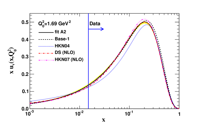
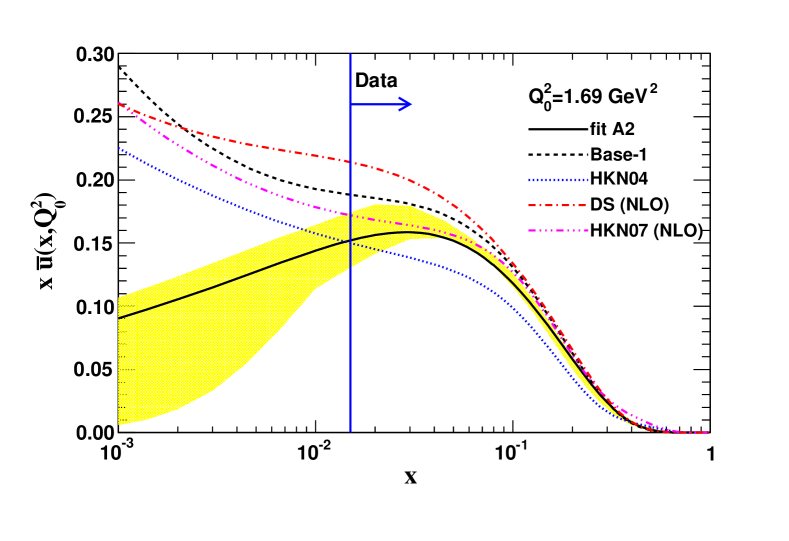
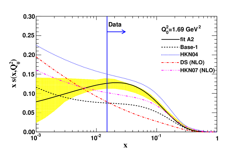
We now examine the nuclear (iron) parton distributions $f_{i}^{A}(x,Q^{2})$ in Figure 1 which shows the PDFs from fit ‘A2’ at our input scale $Q_{0}=m_{c}=1.3\leavevmode\nobreak\ {\rm GeV}$ versus $x$. For an almost isoscalar nucleus like iron the $u$ and $d$ distributions are very similar. Therefore, we only show the $u_{v}$ and $\bar{u}$ partons, together with the strange sea. As explained above, the gluon distribution is very similar to the familiar CTEQ6M gluon at the input scale such that we don’t show it here. In order to indicate the constraining power of the NuTeV data, the band of reasonable fits is depicted. The fits in this band were obtained (as outlined above) by varying the initial conditions and the number of free parameters to fully explore the solution space. All the fits shown in the band have $\chi^{2}/DOF$ within 0.02, which roughly corresponds to a range of $\Delta\chi^{2}\sim 50$ for the 2691 data points.

As can be seen in Figure 1, the $u_{v}$ distribution has a very narrow band across the entire $x$-range. The up- and strange-sea distributions are less precisely determined. At values of $x$ down to, say, $x\simeq 0.07$ the bands are still reasonably well confined; however, they open up widely in the small-$x$ region. Cases where the strange quark sea lies above the up-quark sea are unrealistic, but are present in some of the fits since this region ($x\lesssim 0.02$) is not constrained by data. We have included the curves for our free-proton Base-1 PDFs (dashed), as well as the HKN04 [7] (dotted), the NLO HKN07 [8] (dotted-dashed), and DS [14] (dot-dashed) nuclear PDFs.

The comparison with the Base-1 PDFs is straightforward since the same theoretical framework (input scale, functional form, NLO evolution) has been utilized for their determination. Therefore, the differences between the solid band (‘A2’) and the dashed line (Base-1) exhibit the nuclear effects, keeping in mind that the free-proton PDFs themselves have uncertainties.

For the comparison with the HKN04 distributions, it should be noted that a SU(3)-flavor symmetric sea has been used; therefore, the HKN04 strange quark distribution is larger, and the light quark sea smaller, than their Base-1 PDF counterparts over a wide range in $x$. Furthermore, the HKN04 PDFs are evolved at leading order.

In a recent analysis, the HKN group has published a new set of NPDFs (HKN07) including uncertainties [8]. They provide both LO and NLO sets of PDFs, and we display the NLO set. These PDFs also use a more general set of sea distributions such that $\bar{u}(x)\not=\bar{d}(x)\not=\bar{s}(x)$ in general.

The DS PDFs are linked to the GRV98 PDFs [27] with a rather small radiatively generated strange sea distribution. Consequently, the light quark sea is enhanced compared to the other sets. Additionally, the DS sets are evolved in a 3-fixed-flavor scheme in which no charm parton is included in the evolution. However, at the scale $Q=m_{c}$ of Fig. 1 this is of no importance.

4 Nuclear Correction Factors

In the previous section we analyzed charged current $\nu$–Fe data with the goal of extracting the iron nuclear parton distribution functions. In this section, we now compare our iron PDFs with the free-proton PDFs (appropriately scaled) to infer the proper heavy target correction which should be applied to relate these quantities.

Within the parton model, a nuclear correction factor $R[{\cal O}]$ for an observable ${\cal O}$ can be defined as follows:

$$R[{\cal O}]=\frac{{\cal O}[{\rm NPDF}]}{{\cal O}[{\rm free}]}$$ (1)

where ${\cal O}[{\rm NPDF}]$ represents the observable computed with nuclear PDFs, and ${\cal O}[{\rm free}]$ is the same observable constructed out of the free nucleon PDFs. Clearly, $R$ can depend on the observable under consideration simply because different observables may be sensitive to different combinations of PDFs.

This means that the nuclear correction factor $R$ for $F_{2}^{A}$ and $F_{3}^{A}$ will, in general, be different. Additionally, the nuclear correction factor for $F_{2}^{A}$ will yield different results for the charged current $\nu$–$Fe$ process ($W^{\pm}$ exchange) as compared with the neutral current $\ell^{\pm}$–$Fe$ process ($\gamma$ exchange). Schematically, we can write the nuclear correction for the DIS structure function $F_{2}$ in a charged current (CC) $\nu$–$A$ process as:

$$R_{CC}^{\nu}(F_{2};x,Q^{2}) \simeq \frac{d^{A}+\bar{u}^{A}+...}{d^{{\,\emptyset}}+\bar{u}^{{\,\emptyset}}+...}$$ (2)

and contrast this with the neutral current (NC) $\ell^{\pm}$–$A$ process:

$$R_{NC}^{e,\mu}(F_{2};x,Q^{2})\simeq\qquad\qquad\qquad\qquad\qquad\qquad$$

$$\frac{\left(-\frac{1}{3}\right)^{2}\left[d^{A}+\bar{d}^{A}+...\right]+\left(+\frac{2}{3}\right)^{2}\left[u^{A}+\bar{u}^{A}+...\right]}{\left(-\frac{1}{3}\right)^{2}\left[d^{{\,\emptyset}}+\bar{d}^{{\,\emptyset}}+...\right]+\left(+\frac{2}{3}\right)^{2}\left[u^{{\,\emptyset}}+\bar{u}^{{\,\emptyset}}+...\right]}\ ,$$

where the superscript “${\,\emptyset}$” denotes the “free nucleon” PDF which is constructed via the relation:

$$f_{i}^{{\,\emptyset}}(x,Q)=\frac{Z}{A}\ f_{i}^{p}(x,Q)+\frac{(A-Z)}{A}\ f_{i}^{n}(x,Q)\quad.$$ (3)

Clearly, the $R$-factors depend on both the kinematic variables and the factorization scale. Finally, we note that Eq. (1) is subject to uncertainties of both the numerator and the denominator.

We will now evaluate the nuclear correction factors for our extracted PDFs, and compare these with selected results from the literature [28, 29]. Because we have extracted the iron PDFs from only iron data, we do not assume any particular form for the nuclear $A$-dependence; hence the extracted $R[{\cal O}]$ ratio is essentially model independent.

4.1 $F_{2}^{Fe}/F_{2}^{D}$ NC charged lepton scattering

Figure 2: Parameterization for the neutral current charged lepton structure function $F_{2}^{Fe}/F_{2}^{D}$. For comparison we show experimental results from the BCDMS collaboration (BCDMS-85 [30], BCDMS-87 [31]) and from experiments at SLAC (SLAC-E049 [32], SLAC-E139 [3], and SLAC-E140 [24]). Normalization uncertainties of the data have not been included.

We will also find it instructive to compare our results with the $F_{2}^{{\rm Fe}}/F_{2}^{{\rm D}}$ as extracted in neutral current charged-lepton scattering, $\ell^{\pm}$–$Fe$. In Fig. 2 we compare the experimental results for the structure function ratio $F_{2}^{{\rm Fe}}/F_{2}^{{\rm D}}$ for the following experiments: BCDMS-85 [30], BCDMS-87 [31], SLAC-E049 [32], SLAC-E139 [3], SLAC-140 [24]. The curve (labeled SLAC/NMC parameterization) is a fit to this data. While there is a spread in the individual data points, the parameterization describes the bulk of the data at the level of a few percent or better. It is important to note that this parameterization is independent of atomic number $A$ and the energy scale $Q^{2}$ [33]; this is in contrast to the results we will derive using the PDFs extracted from the nuclear data. Additionally, we note that while this parameterization has been extracted using ratios of $F_{2}$ structure functions, it is often applied to other observables such as $F_{1,3,L}$ or $d\sigma$. We can use this parameterization as a guide to judge the approximate correspondence between this neutral current (NC) charged lepton DIS data and our charged current (CC) neutrino DIS data.

4.2 R Factors for $d^{2}\sigma/dx\,dQ^{2}$

Figure 3: Nuclear correction factor $R$ for the differential cross section $d^{2}\sigma/dx\,dQ^{2}$ in charged current neutrino-Fe scattering at $Q^{2}=5\leavevmode\nobreak\ {\rm GeV}^{2}$. Results are shown for the charged current neutrino (solid lines) and anti-neutrino (dashed lines) scattering from iron. The upper (lower) pair of curves shows the result of our analysis with the Base-2 (Base-1) free-proton PDFs.

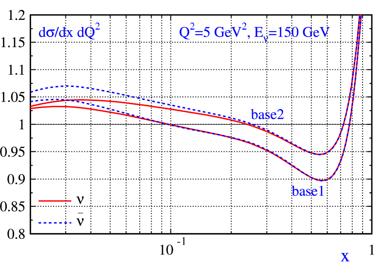
We begin by computing the nuclear correction factor $R$ according to Eq. (1) for the neutrino differential cross section as this represents the bulk of the NuTeV data included in our fit. More precisely, we show $R$-factors for the charged current cross sections $d^{2}\sigma/dx\,dQ^{2}$ at fixed $Q^{2}$. Our results are displayed in Fig. 3 for $Q^{2}=5\leavevmode\nobreak\ {\rm GeV}^{2}$ and a neutrino energy $E_{\nu}=150\ {\rm GeV}$ which implies, due to the relation $Q^{2}=2ME_{\nu}xy$, a minimal $x$-value of $x_{{\rm min}}=0.018$. The solid (dashed) lines correspond to neutrino (anti-neutrino) scattering using the iron PDFs from the ‘A2’ fit.

We have computed $R$ using both the Base-1 and Base-2 PDFs for the denominator of Eq. (1); recall that Base-1 includes a deuteron correction while Base-2 uses the CCFR data and does not include a deuteron correction. The difference between the Base-1 and Base-2 curves is approximately 2% at small $x$ and grows to 5% at larger $x$, with Base-2 above the Base-1 results. The difference of these curves, in part, reflects the uncertainty introduced by the proton PDF.[2] As this behavior is typical, in the following plots (Figs. 4) we will only show the Base-1 results. We also observe that the neutrino (anti-neutrino) results coincide in the region of large $x$ where the valence PDFs are dominant, but differ by a few percent at small $x$ due to the differing strange and charm distributions.

4.3 R Factors for $F_{2}^{\nu}(x,Q^{2})$ and $F_{2}^{\bar{\nu}}(x,Q^{2})$

Figure 4: Nuclear correction factor $R$ for the structure function $F_{2}$ in neutrino and anti-neutrino scattering from Fe for $Q^{2}=\{5,20\}$ GeV². The solid curve shows the result of our analysis of NuTeV data; the uncertainty from the fit is represented by the shaded (yellow) band. For comparison we show the correction factor from the Kulagin–Petti model (dashed-dot line),[28] HKN07 (dashed-dotted line),[8] and the SLAC/NMC parametrization (dashed line).

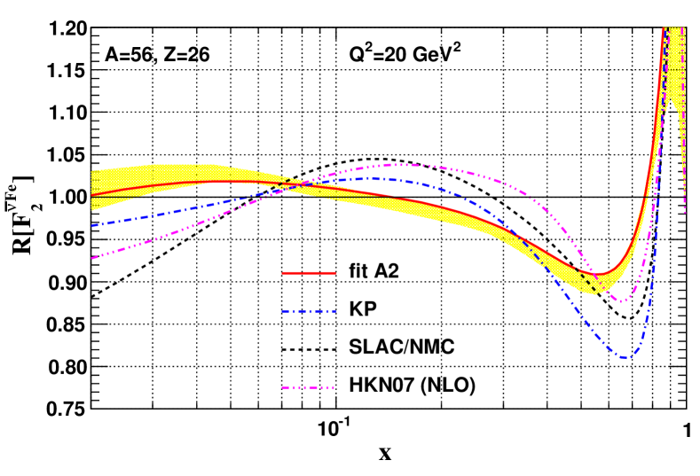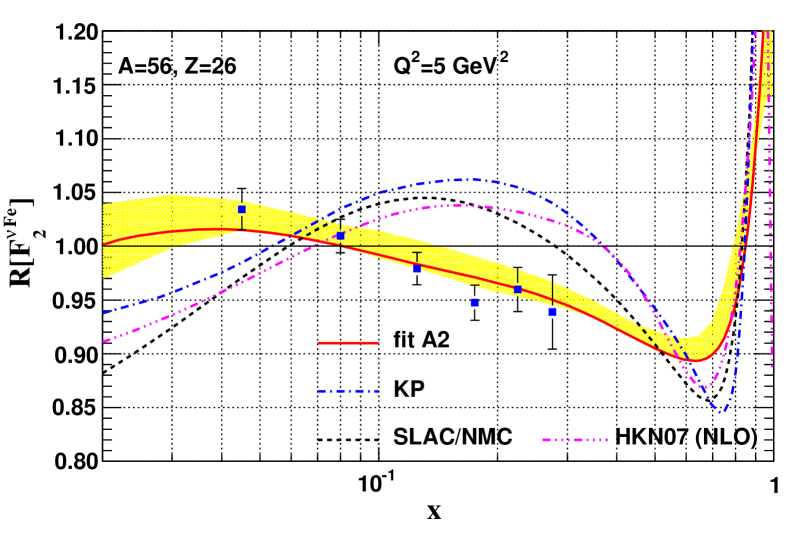
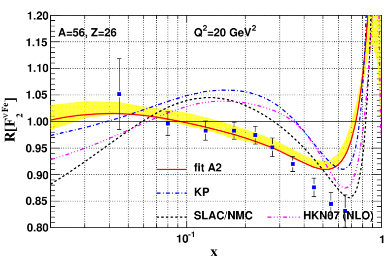
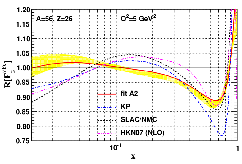
We now compute the nuclear correction factors for charged current neutrino–iron scattering. The results for $\nu$–$Fe$ and those of $\bar{\nu}$–$Fe$ are shown in Fig. 4. The numerator in Eq. (1) has been computed using the nuclear PDF from fit ‘A2’, and for the denominator we have used the Base-1 PDFs. For comparison we also show the correction factor from the Kulagin–Petti model [28, 29] (dashed-dotted), and the SLAC/NMC curve (dashed) which has been obtained from an $A$ and $Q^{2}$-independent parameterization of calcium and iron charged–lepton DIS data.

Due to the neutron excess in iron, both our curves and the KP curves differ when comparing scattering for neutrinos and anti-neutrinos; the SLAC/NMC parameterization is the same in both figures. For our results (solid lines), the difference between the neutrino and anti-neutrino results is relatively small, of order $3\%$ at $x=0.6$. Conversely, for the KP model (dashed-dotted lines) the $\nu$–$\bar{\nu}$ difference reaches $10\%$ at $x\sim 0.7$, and remains sizable at lower values of $x$.

To demonstrate the dependence of the $R$ factor on the kinematic variables, in Fig. 4 we have plotted the nuclear correction factor for two separate values of $Q^{2}$. Again, our curves and the KP model yield different results for different $Q^{2}$ values, in contrast to the SLAC/NMC parameterization.

Comparing the nuclear correction factors for the $F_{2}$ structure function with those obtained for the differential cross section (Fig. 3), we see these are quite different, particularly at small $x$. Again, this is because the cross section $d^{2}\sigma$ is comprised of a different combination of PDFs than the $F_{2}$ structure function. In general, our $R$-values for $F_{2}$ lie below those of the corresponding $R$-values for the cross section $d\sigma$ at small $x$. Since $d\sigma$ is a linear combination of $F_{2}$ and $F_{3}$, the $R$-values for $F_{3}$ (not shown) therefore lie above those of $F_{2}$ and $d\sigma$. Again, we emphasize that it is important to use an appropriate nuclear correction factor which is matched to the particular observable.

As we observed in the previous section, our results have general features in common with the KP model and the SLAC/NMC parameterization, but the magnitude of the effects and the $x$-region where they apply are quite different. Our results are noticeably flatter than the KP and SLAC/NMC curves, especially at moderate-$x$ where the differences are significant. The general trend we see when examining these nuclear correction factors is that the anti-shadowing region is shifted to smaller $x$ values and any turn-over at low $x$ is minimal given the PDF uncertainties. In general, these plots suggest that the size of the nuclear corrections extracted from the NuTeV data are smaller than those obtained from charged lepton scattering (SLAC/NMC) or from the set of data used in the KP model. We will investigate this difference further in the following section.

4.4 $F_{2}^{Fe}/F_{2}^{D}$ from Iron PDFs

Figure 5: Predictions (solid and dashed line) for the structure function ratio $F_{2}^{Fe}/F_{2}^{D}$ using the iron PDFs extracted from fits to NuTeV neutrino and anti-neutrino data. The SLAC/NMC parameterization is shown with the dot-dashed line. The structure function $F_{2}^{D}$ in the denominator has been computed using either the Base-2 (solid line) or the Base-1 (dashed line) PDFs.

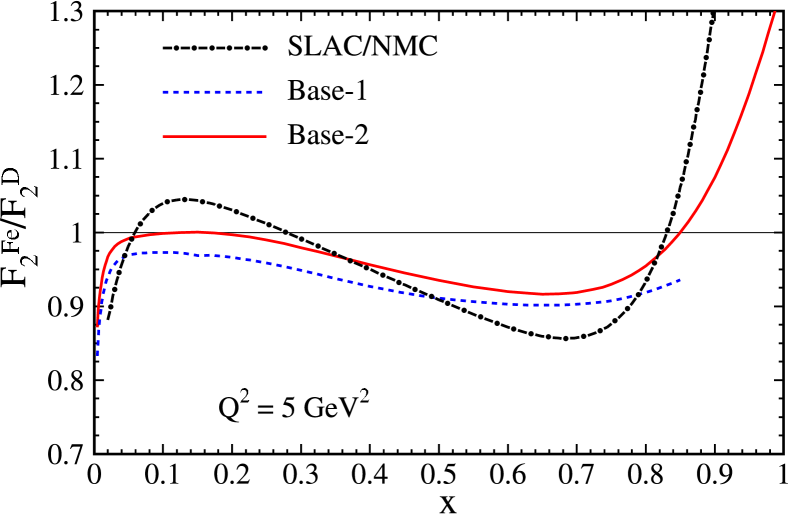
Since the SLAC/NMC parameterization was fit to $F_{2}^{Fe}/F_{2}^{D}$ for charged-lepton DIS data, we can perform a more balanced comparison by using our iron PDFs to compute this same quantity. The results are shown in Fig. 5 where we have used our iron PDFs to compute $F_{2}^{Fe}$, and the Base-1 and Base-2 PDFs to compute $F_{2}^{D}$.

As with the nuclear correction factor results of the previous section, we find our results have some gross features in common while on a more refined level the magnitude of the nuclear corrections extracted from the CC iron data differs from the charged lepton data. In particular, we note that the so-called “anti-shadowing” enhancement at $x\sim[0.06-0.3]$ is not reproduced by the charged current (anti-)neutrino data. Examining our results among all the various $R[{\cal O}]$ calculations, we generally find that any nuclear enhancement in the small $x$ region is reduced and shifted to a lower $x$ range as compared with the SLAC/NMC parameterization. Furthermore, in the limit of large $x$ ($x\gtrsim 0.6$) our results are slightly higher than the data, including the very precise SLAC-E139 points; however,the large theoretical uncertainties on $F_{2}^{D}$ in this $x$-region make it difficult to extract firm conclusions.

This discussion raises the more general question as to whether the charged current ($\nu$–$Fe$) and neutral current ($\ell^{\pm}$–$Fe$) correction factors are entirely compatible [15, 34, 35, 36, 37, 38]. There is a priori no requirement that these be equal; in fact, given that the $\nu$–$Fe$ process involves the exchange of a $W$ and the $\ell^{\pm}$–$Fe$ process involves the exchange of a $\gamma$ we necessarily expect this will lead to differences at some level.

4.5 Future Studies

Figure 6: Illustration of the gluon PDF $x\,f_{g}^{A}(x,\mu)$ vs. $x$ as a function of the nuclear $A$.

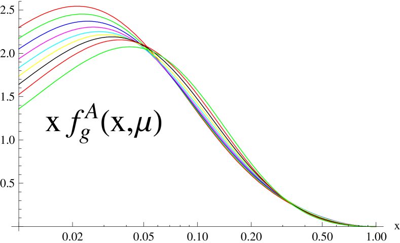
It is important to resolve whether the differences we observe in Fig. 5 arise from the uncertainty of the nuclear corrections, or if they are genuinely a consequence of NC/CC effects. A combined analysis of CC neutrino and NC charged-lepton data sets will shed more light on these issues. To best address these questions, we need to include the nuclear dimension (parameterized by the nuclear A value) as a dynamic component of the global fit; this will allow us to fit both the CC $W^{\pm}$-exchange processes at large A, as well as the NC $\gamma$-exchange processes at small A in a coherent framework. Figure 6 presents an illustrative example of how the PDFs can be extended to incorporate the necessary A dependence to implement such a program. This extended analysis with additional data sets is in progress, and should help clarify these questions.

5 CONCLUSIONS

While the nuclear corrections extracted from charged current $\nu$–$Fe$ scattering have similar characteristics as the neutral current $l^{\pm}$–$Fe$ charged-lepton results, the detailed $x$ and $Q^{2}$ behavior is quite different. This observation raises the deeper question as to whether the charged current and neutral current nuclear correction factors may be substantially different. This present study of the iron PDFs provides a foundation for a general investigation (involving a variable A parameter) that can definitively address this topic. Resolving these questions is essential if we are to reliably use the plethora of nuclear data to obtaining free-proton PDFs which form the basis of the LHC analyses.

References

- [1] J. F. Owens et al. Phys. Rev., D75:054030, 2007.
- [2] I. Schienbein et al. Phys. Rev., D77:054013, 2008.
- [3] J. Gomez et al. Phys. Rev., D49:4348–4372, 1994.
- [4] R. S. Thorne, A. D. Martin, and W. J. Stirling. 2006.
- [5] J. Pumplin et al. JHEP, 07:012, 2002.
- [6] M. Hirai, S. Kumano, and M. Miyama. Phys. Rev., D64:034003, 2001.
- [7] M. Hirai, S. Kumano, and T. H. Nagai. Phys. Rev., C70:044905, 2004.
- [8] M. Hirai, S. Kumano, and T. H. Nagai. Phys. Rev., C76:065207, 2007.
- [9] K. J. Eskola, V. J. Kolhinen, and C. A. Salgado. Eur. Phys. J., C9:61–68, 1999.
- [10] Kari J. Eskola, Vesa J. Kolhinen, Hannu Paukkunen, and Carlos A. Salgado. JHEP, 05:002, 2007.
- [11] M. A. G. Aivazis, Frederick I. Olness, and Wu-Ki Tung. Phys. Rev., D50:3085–3101, 1994.
- [12] M. A. G. Aivazis, John C. Collins, Fredrick I. Olness, and Wu-Ki Tung. Phys. Rev., D50:3102–3118, 1994.
- [13] S. Kretzer and I. Schienbein. Phys. Rev., D58:094035, 1998.
- [14] D. de Florian and R. Sassot. Phys. Rev., D69:074028, 2004.
- [15] M. Tzanov et al. Phys. Rev., D74:012008, 2006.
- [16] M. Goncharov et al. Phys. Rev., D64:112006, 2001.
- [17] E. Oltman et al. Z. Phys., C53:51–71, 1992.
- [18] W. G. Seligman et al. Phys. Rev. Lett., 79:1213–1216, 1997.
- [19] Un-Ki Yang et al. Phys. Rev. Lett., 86:2742–2745, 2001.
- [20] Un-Ki Yang. FERMILAB-THESIS-2001-09.
- [21] H. Abramowicz et al. Z. Phys., C25:29, 1984.
- [22] J. P. Berge et al. Z. Phys., C49:187–224, 1991.
- [23] Janet M. Conrad, Michael H. Shaevitz, and Tim Bolton. Rev. Mod. Phys., 70:1341–1392, 1998.
- [24] S. Dasu et al. Phys. Rev., D49:5641–5670, 1994.
- [25] J. J. Aubert et al. Nucl. Phys., B272:158, 1986.
- [26] J. J. Aubert et al. Nucl. Phys., B293:740, 1987.
- [27] M. Gluck, E. Reya, and A. Vogt. Eur. Phys. J., C5:461–470, 1998.
- [28] S. A. Kulagin and R. Petti. Nucl. Phys., A765:126–187, 2006.
- [29] S. A. Kulagin and R. Petti. Phys. Rev., D76:094023, 2007.
- [30] G. Bari et al. Phys. Lett., B163:282, 1985.
- [31] A. C. Benvenuti et al. Phys. Lett., B189:483, 1987.
- [32] A. Bodek et al. Phys. Rev. Lett., 50:1431, 1983.
- [33] J. Arrington, R. Ent, C. E. Keppel, J. Mammei, and I. Niculescu. Phys. Rev., C73:035205, 2006.
- [34] M. Tzanov. AIP Conf. Proc., 792:241–244, 2005.
- [35] C. Boros, J. T. Londergan, and Anthony William Thomas. Phys. Rev. Lett., 81:4075–4078, 1998.
- [36] C. Boros, Fernando Monti Steffens, J. T. Londergan, and Anthony William Thomas. Phys. Lett., B468:161–167, 1999.
- [37] A. Bodek, Q. Fan, M. Lancaster, K. S. McFarland, and Un-Ki Yang. Phys. Rev. Lett., 83:2892–2895, 1999.
- [38] S. Kretzer, Fredrick I. Olness, R. J. Scalise, R. S. Thorne, and Un-Ki Yang. Phys. Rev., D64:033003, 2001.
- [39] Stanley J. Brodsky, Ivan Schmidt, and Jian-Jun Yang. Phys. Rev., D70:116003, 2004.