Distribution amplitude for the photon-pion transition

Abstract:

The exclusive production of $\pi\pi$ and $\pi\rho$ in hard $\gamma^{\ast}\gamma$ scattering in the forward kinematical region where the virtual photon is highly off-shell are studied through the $\gamma\to\pi^{-}\,$ Transition Distribution Amplitudes. The calculation is based on a covariant Bethe-Salpeter approach, applied to the Nambu - Jona-Lasinio model, for the determination of the pion bound state. In particular it is shown that the pion pole contribution produces a large enhancement of the differential cross section for the pion pair production with respect to previous estimates.

The study of the exclusive meson pair production in $\gamma^{\ast}\gamma$ scattering allows the introduction of a new kind of distribution amplitudes [1]. At small momentum transfer $t$ and in the kinematical regime where the photon is highly virtual, a factorization between the perturbative and the nonperturbative regimes is assumed to be valid. The amplitude for such reactions, represented in Fig. 1, can be written as a convolution of a hard part $M_{h}$, with a meson distribution amplitude $\phi_{M}$ and a soft part describing the photon-pion transition. This soft part is called Transition Distribution Amplitude (TDA).

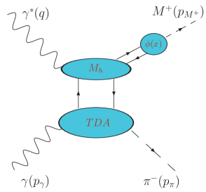
Figure 1: Factorization for the amplitude of the process $\gamma^{\ast}\gamma\rightarrow\pi^{-}M^{+}$ at small momentum transfer.

Cross section estimates for the processes

$$\gamma_{L}^{\ast}\gamma\rightarrow\pi^{+}\pi^{-}\ \ ,\quad\gamma_{L}^{\ast}\gamma\rightarrow\rho^{+}\pi^{-}$$ (1)

have been proposed in Ref. [2] using for the TDA a $t$-independent double distributions, in a first approach, and, in a second, the $t$-dependent results of Ref. [3]. In this paper we evaluate these cross sections in our formalism. To do so we compare results for the TDAs calculated in different realistic models for the pion [4, 5, 6]. Since the results obtained are in agreement, we choose to use the results of a single model calculation, i.e. the NJL model [5]. As shown in Ref. [7], the estimate for the $\pi\pi$ production increases by a factor about 60 due to the presence of the pion pole contribution in our analysis.

1 Transition Distribution Amplitudes

We introduce the light-front vectors $\bar{p}^{\mu}=P^{+}\left(1,0,0,1\right)/\sqrt{2}$ and $n^{\mu}=\left(1,0,0,-1\right)/(\sqrt{2}P^{+})$ where $P^{+}$ is the plus componente of the vector $P=\left(p_{\pi}+p_{\gamma}\right)/2$. The momentum transfer is defined as $\Delta=p_{\pi}-p_{\gamma}$, with $t=\Delta^{2}$ and $P^{2}=m_{\pi}^{2}/2-t/4$. The skewness variable describes the loss of plus momentum of the incident photon, i.e. $\xi=\left(p_{\gamma}-p_{\pi}\right)^{+}/2P^{+},$ and its value ranges between $-1<\xi<-t/\left(2m_{\pi}^{2}-t\right)$. With these conventions, the vector and axial TDA are defined by

$$\int\frac{dz^{-}}{2\pi}e^{ixP^{+}z^{-}}\left.\left\langle\pi^{\pm}(p_{\pi})\right|\bar{q}\left(-\frac{z}{2}\right)\gamma^{+}\tau^{\pm}\ q\left(\frac{z}{2}\right)\left|\gamma(p_{\gamma}\varepsilon)\right\rangle\right|_{z^{+}=z^{\bot}=0}$$

$$=\frac{1}{P^{+}}\ i\,e\,\varepsilon_{\nu}\,\epsilon^{+\nu\rho\sigma}\,P_{\rho}\,(p_{\pi}-p_{\gamma})_{\sigma}\,\frac{V^{\gamma\rightarrow\pi^{\pm}}(x,\xi,t)}{\sqrt{2}f_{\pi}}\quad,$$

(2)

$$\int\frac{dz^{-}}{2\pi}e^{ixP^{+}z^{-}}\left.\left\langle\pi^{\pm}\left(p_{\pi}\right)\right|\bar{q}\left(-\frac{z}{2}\right)\gamma^{+}\gamma_{5}\ \tau^{\pm}\ q\left(\frac{z}{2}\right)\left|\gamma\left(p_{\gamma}\varepsilon\right)\right\rangle\right|_{z^{+}=z^{\bot}=0}$$

$$=\pm\ \frac{1}{P^{+}}\left[-\ e\,\left(\vec{\varepsilon}^{\bot}\cdot(\vec{p}_{\pi}^{\bot}-\vec{p}_{\gamma}^{\bot})\right)\frac{A^{\gamma\rightarrow\pi^{\pm}}(x,\xi,t)}{\sqrt{2}f_{\pi}}\right.\left.+\ e\,\left(\varepsilon\cdot(p_{\pi}-p_{\gamma})\right)\frac{2\sqrt{2}f_{\pi}}{m_{\pi}^{2}-t}~{}\epsilon(\xi)~{}\phi_{\pi}\left(\frac{x+\xi}{2\xi}\right)\right].$$

(3)

where the pion decay constant is $f_{\pi}=92.4$ MeV, $\epsilon\left(\xi\right)$ is equal to $1$ for $\xi>0$ and to $-1$ for $\xi<0$ and $\phi_{\pi}(x)$ is the pion DA. Here we have modified the definition given in [1, 2] in order to introduce the pion pole contribution in the Eq. (3) [3, 5]. This pion pole term describes a point-like pion propagator multiplied by the distribution amplitude (DA) of an on-shell pion. It contributes to the axial current through a different momentum structure and must be subtracted in order to obtain de axial TDA. With these -model independent- definitions we recover the sum rules

$$\int_{-1}^{1}dx\ D\left(x,\xi,t\right)=\frac{\sqrt{2}\ f_{\pi}}{m_{\pi}}\ F_{D}\left(t\right)\ \ \ ,\ \ \ \ \ \ \ \ \ \ \ \ \ \ \ D=V,A$$ (4)

with the standard definitions for the form factors $F_{V,A}$ appearing in the $\pi^{\pm}\rightarrow\ell^{\pm}\nu\gamma$ decay [8]. Notice that the on-shell pion DA obeys the normalization condition $\int_{0}^{1}dx\,\phi_{\pi}(x)=1$. A model calculation for $A\left(x,\xi,t\right)$ implies the evaluation of all diagrams contributing to the matrix element of the axial current and to extract from this result the pion pole contribution calculated in the same model.

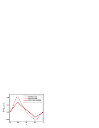
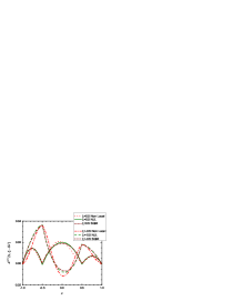
Figure 2: The $\pi^{+}$-$\gamma$ TDAs for $t=-0.1$ GeV² of Refs. [4, 6] for $m_{\pi}=0$ MeV and Ref. [5] for $m_{\pi}=140$ MeV. On the left, the vector TDA for $\xi=\pm 0.5$ as a single (solid) curve for the results of both the NJL model and SQM (these four curves are indistinguishable); the result of the non-local $\chi$QM calculation for $\xi=0.5$ (dotted line) and for $\xi=-0.5$ (dashed-dotted line). On the right, the axial TDA.

Recently the pion-photon TDAs have been calculated in the Spectral Quark Model (SQM) [4], the Nambu - Jona-Lasinio model with Pauli-Villars regularization procedure (NJL) [5] and a nonlocal chiral quark model ($\chi$QM) [6]. A comparison of the TDAs obtained in these three models has been shown in Ref. [9]. We here recall the conclusion of the comparison by plotting the different results for the $\pi^{+}\to\gamma$ transition in Fig. 2. There is good agreement between the different studies of the pion-photon TDAs in spite of the discrepancy coming from the vector TDA for a negative $\xi$ in the non-local $\chi$QM. Thus, in the present analysis, we can concentrate on the TDAs obtained in a single model, e.g. the NJL model [5]. The $\gamma$-$\pi$ TDAs defined in Eqs. (2-3) are connected to the $\pi$-$\gamma$ TDAs through the $T$ or $CPT$ symmetries; we find [9]

$$D^{\gamma\rightarrow\pi^{+}}\left(x,\xi,t\right)=D^{\pi^{+}\rightarrow\gamma}\left(x,-\xi,t\right)\quad\&\quad D^{\gamma\rightarrow\pi^{-}}\left(x,\xi,t\right)=D^{\pi^{+}\rightarrow\gamma}\left(-x,-\xi,t\right)\quad,$$ (5)

with $D=V,A$.

2 Exclusive meson production in $\gamma^{\ast}\gamma$ scattering: Cross section estimates

The $\gamma^{\ast}\gamma\rightarrow M^{+}\pi^{-}$ processes, with $M=\rho_{L}$ or $\pi$, are subprocesses of the $e\left(p_{e}\right)+\gamma\left(p_{\gamma}\right)\rightarrow e\left(p_{e}^{\prime}\right)+M^{+}\left(p_{M}\right)+\pi^{-}\left(p_{\pi}\right)$ processes. We follow all the kinematics given in Section III. A and Fig. 3 of Ref. [2], but with $n.p=1$. In particular, for massless pions,

$$Q^{2}=-q^{2}=-\left(p_{e}-p_{e}^{\prime}\right)^{2}\quad,\qquad s_{e\gamma}=\left(p_{e}+p_{\gamma}\right)^{2}\quad,$$ (6)

$$p_{\gamma}=(1+\xi)\bar{p},\quad p_{\pi}=(1-\xi)\bar{p}+\frac{\vec{\Delta}^{\perp 2}}{2\left(1-\xi\right)}n+\vec{\Delta}^{\perp},$$

$$q=-2\xi\bar{p}+\frac{Q^{2}}{4\xi}n\quad,$$

where $\Delta_{T}=(0,\vec{\Delta}^{\perp},0)$ and therefore $\Delta_{T}^{2}=-\vec{\Delta}^{\perp 2}$. Notice that $\vec{\Delta}^{\perp 2}=(-t)(1-\xi)/(1+\xi)$, with $t<0$. The longitudinal polarization of the incoming virtual photon is defined through the conditions $\varepsilon_{L}^{2}=1$ and that $\varepsilon_{L}.q=0$,

$$\varepsilon_{L}=\left(\frac{2\xi}{Q}\bar{p}+\frac{Q}{4\xi}n\right)\quad;$$

while the real photon polarization is defined by $\varepsilon\cdot p_{\gamma}=0$, which leads to $\varepsilon^{-}=0$ together with the gauge condition $\varepsilon^{+}=0$.

The differential cross sections are given by [2]

$$\frac{d\sigma^{e\gamma\to e\rho_{L}^{+}\pi^{-}}}{dQ^{2}dtd\xi} = \frac{64\pi^{2}}{9}\,\frac{\alpha_{elm}^{3}}{s_{e\gamma}\,Q^{8}}\,(-t)\,\frac{1-\xi}{(1+\xi)^{4}}\,\left(2\xi\,s_{e\gamma}\,-\,(1+\xi)Q^{2}\right)\,\left\{\Re^{2}{I}_{x}^{\rho}+\Im^{2}{I}_{x}^{\rho}\right\};$$

$$\frac{d\sigma^{e\gamma\to e\pi^{+}\pi^{-}}}{dQ^{2}dtd\xi} = \frac{64\pi^{2}}{9}\,\frac{\alpha_{elm}^{3}}{s_{e\gamma}\,Q^{8}}(-t)\frac{1-\xi}{(1+\xi)^{4}}\left(2\xi s_{e\gamma}-(1+\xi)Q^{2}\right)\left\{\left(\Re{I}_{x}^{\pi}-\frac{3}{4\pi}\frac{Q^{2}\,F_{\pi}\left(Q^{2}\right)}{t-m_{\pi}^{2}}\right)^{2}+\Im^{2}{I}_{x}^{\pi}\right\},$$

(8)

with

$${I}_{x}^{\rho} = \frac{\alpha_{s}}{6}\int_{-1}^{1}dx\,\int_{0}^{1}dz\,\left(\frac{f_{\rho}}{\sqrt{2}\,f_{\pi}}\right)\,\phi_{\rho}(z)\,\frac{1}{z(1-z)}\left(\frac{Q_{u}}{x-\xi+i\epsilon}+\frac{Q_{d}}{x+\xi-i\epsilon}\right)V(x,\xi,t)\quad;$$ (9)

$${I}_{x}^{\pi} = \frac{\alpha_{s}}{6}\int_{-1}^{1}dx\,\int_{0}^{1}dz\,\phi_{\pi}(z)\,\frac{1}{z(1-z)}\left(\frac{Q_{u}}{x-\xi+i\epsilon}+\frac{Q_{d}}{x+\xi-i\epsilon}\right)A(x,\xi,t)\quad,$$ (10)

where $z$ is the light-cone momentum fraction carried by the quark entering the meson $M^{+},$ $f_{\rho}=0.216$ GeV. The term proportional to $F_{\pi}$ on the r.h.s. of Eq. (8) is the pion pole contribution to the amplitude coming from the second term of Eq. (3).

From Eqs. (2-8) it can be observed that $\xi\geq Q^{2}/\left(2s_{e\gamma}-Q^{2}\right)$. In other words, there is a (positive) lower limit on the value of $\xi$. It is indeed a particularly interesting restriction because the sign of $\xi$ defines the shape of the axial TDA.

We proceed now to the evaluation of the integrals (9-10). The meson DA, $\phi_{M}\left(z\right),$ is chosen to be the usual asymptotic normalized meson DA, i.e. $\phi_{M}(z)=6z(1-z)$, what cancels the $z$-dependence of the hard amplitude. Because of the non perturbative information they contain, the TDAs have to be evaluated in a model. We here focus on the TDAs calculated in the NJL model [5]. This approach is based on the determination of the pion as a bound state through the Bethe-Salpeter equation, what guarantees the preservation of all the invariances of the problem. As a consequence, the obtained TDAs explicitly verify the sum rules, the polynomiality condition and have the correct support in $x$. The NJL model gives a good description of the low energy pion physics [11] and it has already been applied to the study of the pion parton distribution (PD) [12] and the pion generalized parton distribution (GPD) [13]. Once evolution is taken into account, the calculated PD is in good agreement with the experimental one [12]. The QCD evolution of the pion GPD calculated in the NJL model has been studied in [14]. More elaborated studies of the pion PD has been done in, e.g., the Instanton Liquid Model [15], lattice calculation based models [17] using non local lagrangians [16], which confirms that the result obtained in the NJL model for the PD is a good approximation. It is therefore of interest to obtain the cross sections for the processes (1) in such a realistic model.

In order to numerically estimate the cross sections, we need to fix the strong coupling constant $\alpha_{s}$. In Ref. [18] it is indicated that a large value of $\alpha_{s}$ ($\alpha_{s}=1$) should be used together with the asymptotic DA. We hence use the value $\alpha_{s}=1$.

The result for the cross section for $\rho$ production is shown in Fig. 3 as a function of $\xi$. The cross section is largely dominated by the imaginary part (dotted line) of the integral of Eq. (9). Comparing with the previous obtained results in Ref. [2], we observe that our predictions are higher by a factor 2 or 3.

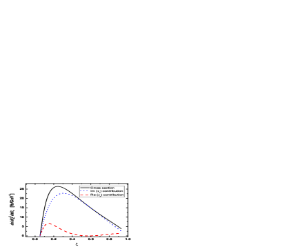
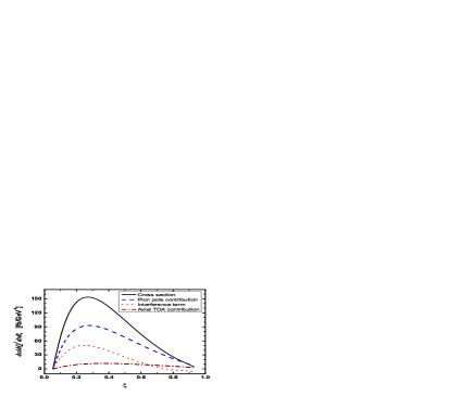
Figure 3: The $e\gamma\rightarrow e^{\prime}M^{+}\pi^{-}$ differential cross section with $M=\rho_{L}$ on the left and $M=\pi$ on the right. The plots are given as functions of $\xi$ for $Q^{2}=4$ GeV${}^{2},$ $s_{e\gamma}=40$ GeV${}^{2},$ $t=-0.5$ GeV².

The $\pi\pi$ production is described by Eq. (8). The pion pole term of the axial current leads to a contribution proportional to the pion form factor $F_{\pi}(Q^{2})$. If we use the asymptotic form of the pion DA, $\phi_{\pi}\left(z\right)$ with $z=\left(x+\xi\right)/2\xi,$ for the evaluation of this contribution we obtain the Brodsky-Lepage result for $F_{\pi}(Q^{2})$,

$$\frac{3}{4\pi}Q^{2}\,F_{\pi}\left(Q^{2}\right)=12\,\alpha_{s}f_{\pi}^{2}$$ (11)

The cross section for pion production as a function of $\xi$ is given on the right of Fig. 3. We notice an enhancement of about 2 orders of magnitude [7] with respect to the first estimates given in Ref. [2], due to the presence of the pion pole in Eq. (8). The cross section is indeed dominated by the pion pole contribution (dashed line) whose behavior is governed by the pion FF. The latter being experimentally determined, the pion pole contribution is perfectly known. Thus one could extract information about the axial TDA from the interference term (dotted line) whose contribution is more important than the pure axial TDA’s contribution (dotted-dashed line).

We finally remark that, contrary to the contributions coming from the TDAs, the pion pole strongly depends on the momentum transfer for small values of $t$. Neglecting the pion mass, the cross section for this contribution goes like $t^{-1}$. For large values of $t$ the behaviour of all contributions is as $t^{-1}$.

- [1] B. Pire and L. Szymanowski, Hadron annihilation into two photons and backward VCS in the scaling regime of QCD, Phys. Rev. D71 (2005) 111501 [hep-ph/0411387].
- [2] J. P. Lansberg, B. Pire and L. Szymanowski, Exclusive meson pair production in gamma* gamma scattering at small momentum transfer, Phys. Rev. D73 (2006) 074014 [hep-ph/0602195].
- [3] B. C. Tiburzi, Estimates for pion photon transition distributions, Phys. Rev. D72 (2005) 094001 [hep-ph/0508112].
- [4] W. Broniowski and E. R. Arriola, Pion photon transition distribution amplitudes in the spectral quark model, Phys. Lett. B649 (2007) 49 [hep-ph/0701243].
- [5] A. Courtoy and S. Noguera, The Pion-Photon Transition Distribution Amplitudes in the Nambu-Jona Lasinio Model, Phys. Rev. D76, 094026 (2007) [0707.3366 [hep-ph]].
- [6] P. Kotko and M. Praszalowicz, Pion-to-photon transition distribution amplitudes in the non-local chiral quark model, [0803.2847 [hep-ph]].
- [7] A. Courtoy and S. Noguera, Enhancement effect in exclusive pion production in scattering, (in preparation).
- [8] C. Amsler et al. [Particle Data Group], Review of particle physics, Phys. Lett. B667 (2008) 1.
- [9] A. Courtoy and S. Noguera, Pion-Photon Transition Distribution Amplitudes, [arXiv:0804.4337 [hep-ph]]
- [10] J. P. Lansberg, Private communication.
- [11] S. P. Klevansky, The Nambu-Jona-Lasinio model of quantum chromodynamics, Rev. Mod. Phys. 64 (1992) 649.
- [12] R. M. Davidson and E. Ruiz Arriola, Structure Functions Of Pseudoscalar Mesons In The SU(3) Njl Model, Phys. Lett. B348 (1995) 163; Parton distributions functions of pion, kaon and eta pseudoscalar mesons in the NJL model, Acta Phys. Polon. B33 (2002) 1791 [arXiv:hep-ph/0110291].
- [13] S. Noguera, L. Theussl and V. Vento, Generalized parton distributions of the pion in a Bethe-Salpeter approach, Eur. Phys. J. A20 (2004) 483 [nucl-th/0211036].
- [14] W. Broniowski, E. R. Arriola and K. Golec-Biernat, Generalized parton distributions of the pion in chiral quark models and their QCD evolution, Phys. Rev. D77 (2008) 034023. [arXiv:0712.1012 [hep-ph]].
- [15] I. V. Anikin, A. E. Dorokhov and L. Tomio, Pion structure in the instanton liquid model, Phys. Part. Nucl. 31, 509 (2000) [Fiz. Elem. Chast. Atom. Yadra 31, 1023 (2000)].
- [16] S. Noguera, Non local lagrangians. I: The pion, Int. J. Mod. Phys. E16 (2007) 97 [hep-ph/0502171].
- [17] S. Noguera and V. Vento, Pion parton distributions in a non local Lagrangian, Eur. Phys. J. A28 (2006) 227 [hep-ph/0505102].
- [18] V. M. Braun, A. Lenz, G. Peters and A. V. Radyushkin, Light cone sum rules for gamma* N –¿ Delta transition form factors, Phys. Rev. D73 (2006) 034020 [arXiv:hep-ph/0510237].