Minimum entropy production closure of the photo-hydrodynamic equations for radiative heat transfer

Abstract

In the framework of a two-moment photo-hydrodynamic modelling of radiation transport, we introduce a concept for the determination of effective radiation transport coefficients based on the minimization of the local entropy production rate of radiation and matter. The method provides the nonequilibrium photon distribution from which the effective absorption coefficients and the variable Eddington factor (VEF) can be calculated. The photon distribution depends on the frequency dependence of the absorption coefficient, in contrast to the distribution obtained by methods based on entropy maximization. The calculated mean absorption coefficients are not only correct in the limit of optically thick and thin media, but even provide a reasonable interpolation in the cross-over regime between these limits, notably without introducing any fit parameter. The method is illustrated and discussed for grey matter and for a simple example of non-grey matter with a two-band absorption spectrum. The method is also briefly compared with the maximum entropy concept.

I Introduction

Excessive effort is required for modelling and simulation of radiation heat transfer in media with complex optical absorption spectra, like hot gases or plasma Tien1968 . If the radiation model is part of a larger model for hot, compressible mixtures of various chemically reacting species consisting of complex ions, electrons, neutral molecules etc., and subject to transonic and turbulent flow, an exact treatment is not nearly possible. Applications range from arc physics in welding or electrical switching Jones1980 ; Eby1998 ; Nordborg2008 , atomic explosions, up to astrophysics Goupil1984 . A frequently used approximate radiation model is photo-hydrodynamics, which is based on a two-moment expansion of the radiative transfer equation and a variable Eddington factor (VEF) closure Levermore1984 . This concept can even be realized in a multiband framework, where the relevant quantities are decomposed according to their spectral properties Ripoll2008 .
The main problem of photo-hydrodynamic models is the optimal choice of the effective transport parameters, i.e., the effective absorption coefficients and the Eddington factor, which generally depend on the hydrodynamic and thermodynamic variables. The most prominent examples are the Planck mean absorption coefficient for optically thin media, the corresponding Rosseland mean for optically thick media SiegelHowell1992 , and the constant Eddington factor of $1/3$ for isotropic radiation.
Besides these special limit cases, the optimal definition of effective transport parameters is not straightforward Ripoll2001 ; Ripoll2004 . Accurate treatment of the general case is particularly important when radiation in the cross-over range between optically thin and thick limit dominates the physical behavior of a system, or if a medium is simultaneously transparent and opaque for different relevant wavelength bands. A simple approximate approach to solve that problem can consist in the construction of fitting expressions that interpolate between the limit cases. This has been done, for instance, by Sampson Sampson1965 for the absorption coefficient and by Kershaw Kershaw1976 for the variable Eddington factor. Another suggestion by Patch Patch1967 generalizes heuristically averages, which are exact for special cases. A very common approach is based on entropy maximization Levermore1984 ; Minerbo1977 ; Anile1991 . However, Struchtrup StruchtrupUP has pointed out a weakness of this procedure due to the neglect of the of radiation-matter coupling for the determination of the nonequilibrium photon distribution function, which plays indeed a main role for equilibration Planck1906 . One of the consequences is that already the Rosseland mean aborption coefficient in the near-equilibrium case is not correctly reproduced by a two-moment photo-hydrodynamics with the maximum entropy closure. In this paper, we propose to use an entropy production rate principle, and we will show that the limit cases are correctly reproduced and the cross-over between them is provided in a natural way, i.e., without further model parameters.

Maximization and minimization of the entropy production rate $\dot{S}$ have turned out to be powerful approaches for modelling many complex nonequilibrium systems Martyushev2006 . We mention that whether the optimum of $\dot{S}$ is a maximum or a minimum depends on the type of constraints Christen2006a and emphasize that entropy production optimization is in general not an exact physical law except near equilibrium, i.e., in linear deviation from equilibrium. However, it often provides useful approximate results even far away from equilibrium, provided a predominance of strongly irreversible equilibration processes. It is also important for the discussion below that the method is not restricted to systems in (partial) local equilibrium, i.e., where the notion of (probably several) local temperatures can be introduced (e.g., electron and ion temperatures in a plasma, light pencil temperatures for radiation Oxenius1966 ; Kroll1967 , etc.). Entropy production optimization has been shown to be applicable to local nonequilibrium systems, for instance to Knudsen layers in material ablation or evaporation processes FordLee2001 ; Christen2007a . In such cases, the notion of entropy can still be defined LandauLifshitz .
Entropy production of radiation has been discussed by Oxenius Oxenius1966 and Kröll Kroll1967 . Various results related to entropy production principles in radiation have been reported. Essex Essex1984 has shown that the entropy production rate is minimum in a grey atmosphere in local radiative equilibrium. Also this author has pointed out that a consideration of the interaction between radiation and matter is crucial because it contains the appropriate equilibration, i.e. entropy production, mechanism. Later on, Würfel and Ruppel WurfelRuppel1985 ; Kabelac1994 discussed entropy production rate maximization by introducing an effective chemical potential of the photons, related to their interaction with matter. Finally, we mention Santillan et al. Santillan1998 who showed that for a constraint of fixed radiation power, the black bodies are those which maximize the entropy production rate.

This paper is organized as follows. In order to fix notation and to introduce the relevant quantities, in Sect. II the photo-hydrodynamic equations are recalled. We will consider a system that is characterized by similar assumptions as in Patch1967 . Scattering as well as photon time of flight effects are assumed to be negligible, the matter is non-relativistic and in thermal equilibrium, and the ordinary index of refraction is unity. Section III provides the basic result, i.e., Eq. (23) determining the non-equilibrium photon distribution function. From this distribution function the transport coefficients can be calculated. In Sect. IV we show that the approach provides the Rosseland mean in the corresponding limit case. In Sect. V cases far from equilibrium are discussed. In particular, the emission limit, grey matter, and a simple artificial but illustrative example for non-grey matter are investigated. Our results are compared with the method of entropy maximization in Sect. VI.

II Photo-Hydrodynamics

We start from the Boltzmann equation (which is equivalent to the radiative transfer equation Tien1968 ) for the photon distribution function $f(\vec{x},\vec{k})$ at location $\vec{x}$ and wave number $\vec{k}=k\vec{s}$, with direction vector $\vec{s}$, $\mid\vec{s}\mid=1$. The function $f$ is related to the spectral radiation intensity (radiance) $I$ by $I=(\omega^{3}/c^{2})\hbar f$, where $c$ is the velocity of light and $\omega=ck$ is the angular frequency. Neglecting scattering, the Boltzmann equation for $f$ reads Tien1968 ; StruchtrupUP (here, in contrast to Ref. Tien1968 , $\kappa(k)$ includes the material density)

$$\partial_{t}f+c\vec{s}\cdot\vec{\nabla}f=-c\kappa(k)(f-f^{(eq)})\;\;.$$ (1)

Assuming that matter is in thermal equilibrium (at temperature $T$), the emission term contains the well-known Planck distribution

$$f^{(eq)}(k)=\frac{y}{\exp(\hbar ck/k_{B}T)-1}\;\;,$$ (2)

with the photon density of states $y=2/(2\pi)^{3}$ including two polarization states. (For a generalization to nonequilibrium matter, e.g., a plasma with separate electron and ion temperatures, the emission term has to be replaced by the appropriate emission source function, and the entropy production of matter has to be treated in an appropriately generalized way.)
In Eq. (1) scattering is neglected, absorption and spontaneous as well as induced emission are taken into account in the spectral absorption coefficient $\kappa(k)=\kappa^{(0)}(k)[1-\exp(-\hbar ck/k_{B}T)]$.
It is well-known that in local equilibrium particle gas dynamics, from the Boltzmann transport equation hydrodynamic balance equations for mass, momentum, and energy balance can be derived. For photons one can proceed in a similar way but with two serious restrictions. First, because the photon number is not conserved, a continuity equation analogous to mass balance will not appear. The first moment is related to the energy, which is proportional to wave number for massless particles. Secondly, because the photon gas is generally not near equilibrium, one should in principle consider a large number of moments of general order and degree StruchtrupUP ; Struchtrup1998 . Although we will restrict the number of moments to two, the entropy production method to be used is principally not limited to a specific number of moments (cf. also StruchtrupWeiss1998 ).
In analogy to the P-N model SiegelHowell1992 , an expansion can be defined in terms of spherical harmonics,

$$f_{lm}=\int d^{3}k\,f(k,\Theta,\varphi)kY_{lm}^{\ast}(\Theta,\varphi),$$ (3)

where $\Theta$ and $\varphi$ are the zenith and azimuthal angle of the vector $\vec{k}$, and the asterisk indicates complex conjugation. $Y_{lm}$ are the usual spherical harmonic functions with indices $l$ and $m$. Here, $l$ gives the order of the moment. Due to the factor $\vec{s}$ in Eq. (1), the equation of motion for moments of order $l$ is linked to moments of order $l+1$. We introduce this notation, because for the analytical calculations below, it is sometimes convenient to use spherical harmonics.
In Cartesian coordinates, the first three moments $f_{lm}$ are associated with energy ($l=0$), momentum ($l=1$), and radiation pressure tensor ($l=2$). Energy (photon energy $\hbar\omega=\hbar ck$) and momentum (photon momentum $\hbar\vec{k}$) densities are defined by

$$e(\vec{x}) = \int d^{3}k\,f\hbar ck\;\;,$$ (4)

$$\vec{p}(\vec{x}) = \int d^{3}k\,f\hbar\vec{s}k\;\;.$$ (5)

The relations of energy and momentum to the moments defined in (3) are, for instance $e=\hbar c\sqrt{4\pi}f_{00}$ and $p_{z}=\hbar\sqrt{4\pi/3}f_{10}$, respectively. Multiplication of Eq. (1) with $\hbar ck$ and $\hbar k\vec{s}$ and integration over momentum space gives

$$\partial_{t}e+c^{2}\vec{\nabla}\cdot\vec{p} = P_{e}\;\;,$$ (6)

$$\partial_{t}\vec{p}+\vec{\nabla}\cdot\Pi = \vec{P}_{p}\;\;,$$ (7)

where $\Pi$ is the pressure tensor of the photon gas, having the components

$$\Pi_{mn}=\int d^{3}k\,s_{m}s_{n}f\hbar ck\;\;.$$ (8)

The radiation pressure is $\Sigma_{n=1}^{3}\Pi_{nn}/3=e/3$. The source terms of Eqs. (6) and (7), which mediate the interaction of radiation with matter, are

$$P_{e} = -\hbar c^{2}\int d^{3}k\,k\kappa(k)(f-f^{(eq)})\;\;,$$ (9)

$$\vec{P}_{p} = -\hbar c\int d^{3}k\,\vec{k}\kappa(k)f\;\;.$$ (10)

The radiative heat production $w(\vec{x})$, which will appear as a source term in the energy balance equation for the matter is given by

$$w=-P_{e}\;\;.$$ (11)

For a closure of two-moment expansion, the pressure tensor $\Pi$ has to be expressed as a function of energy $e$ and momentum $\vec{p}$. Based on tensor symmetry arguments and on the trace requirement, one can show that $\Pi$ has the general form StruchtrupUP

$$\Pi_{mn}=e\left(\frac{1-\chi}{2}\delta_{mn}+\frac{3\chi-1}{2}\frac{p_{m}p_{n}}{p^{2}}\right)\;\;,$$ (12)

where $\chi(e,p)$ (with $p=\mid\vec{p}\mid$) is the so-called variable Eddington factor (VEF) describing radiation anisotropy. If radiation is isotropic (e.g., in the purely diffusive limit) $\Pi$ must be proportional to the identity matrix, which implies $\chi=1/3$. For a beam (e.g., $\vec{p}$ in $z$-direction), however, $\chi=1$ must hold. Therefore, $\chi$ allows to describe non-diffusive, directed radiation. The pressure tensor is related to the second order moments $f_{2m}$. For instance, assuming $\vec{p}$ in $z$-direction, Eq. (8) and $Y_{20}=\sqrt{5/16\pi}(3\cos^{2}(\Theta)-1)$ imply the relation

$$\Pi_{33}=e\,\chi=\frac{1}{3}\left(e+\sqrt{\frac{16\pi}{5}}\hbar cf_{20}\right)\;\;,$$ (13)

which will be needed below. Effective absorption coefficients $\kappa_{e,p}$ can be formally defined by expressing the source terms (9) and (10) by

$$P_{e} = c\kappa_{e}(e^{(eq)}-e)\;\;,$$ (14)

$$\vec{P}_{p} = -c\kappa_{p}\vec{p}\;\;.$$ (15)

The effective absorption coefficients $\kappa_{e,p}(e,p,T)$ generally depend on $e$, $p$, and $T$. Here, $e^{(eq)}$ is the equilibrium energy density

$$e^{(eq)}=\frac{4}{c}\sigma T^{4}\;\;,$$ (16)

where $\sigma=2\pi^{5}k_{B}^{4}/15c^{2}h^{3}\approx 5.67\,10^{-8}\,$W/m²K⁴ is the Stefan-Boltzmann constant. The energy radiated by a blackbody per time and area is given by $\sigma T^{4}=ce^{(eq)}/4$.
Equations (6) and (7) define the photo-hydrodynamic equations for the variables $e$ and $\vec{p}$ of the photon gas. In order to solve a complete radiation problem, Eqs. (6) and (7) must be solved together with the hydrodynamic equations for the matter. This work focuses on the problem of the determination of the yet unknown effective transport coefficients $\kappa_{e,p}$ and $\chi$. For this, the distribution $f(\vec{x},\vec{k})$ must be known. Often simple approximate averages are used involving the equilibrium function $f^{(eq)}$, like the above mentioned Planck mean,

$$\kappa_{\rm Pl}=\frac{\hbar c\int d^{3}k\,\kappa kf^{(eq)}}{e^{(eq)}}\;\;,$$ (17)

and Rosseland mean,

$$\kappa_{\rm Ro}=\frac{\int d^{3}k\,k^{2}\partial_{k}f^{(eq)}}{\int d^{3}k\,\kappa^{-1}k^{2}\partial_{k}f^{(eq)}}\;\;.$$ (18)

While the former is a weighted spectral average of the absorption coefficient $\kappa(k)$ that depends on the wave number $k$, the latter is the inverse of a weighted spectral average of the inverse absorption coefficient $\kappa^{-1}$. The two cases strongly differ as the Planck limit is dominated by wave number bands with large $\kappa(k)$ values, while the Rosseland limit is dominated by small $\kappa(k)$. In the associated limit cases radiation is isotropic and the Eddington factor, being the ratio of pressure and energy density, equals $1/3$.
Prior to the calculation of $f$ and the effective transport coefficients with entropy production minimization, we mention that the issue of photo-hydrodynamic boundary conditions for $e$ and $\vec{p}$ will not be discussed in this paper. We refer the reader to appropriate literature SiegelHowell1992 ; Su2000 .

III Minimization of the Entropy Production Rate

In the following, we determine $f$, and from this $\chi(e,p)$ and $\kappa_{e,p}(e,p)$, by minimizing the total entropy production rate $\dot{S}$ under constraints of fixed values of $e$ and $p$ (we always assume $\vec{p}$ in $z$-direction). First, we derive an expression for the relevant part of the entropy production rate. The radiation entropy is given by (see, e.g., StruchtrupUP )

$$S_{\rm rad}(\vec{x})=-k_{B}\int d^{3}k\Biggl{(}f\ln(f/y)-(y+f)\ln(1+f/y)\Biggr{)}\;\;.$$ (19)

The part of the entropy production rate of the photon gas alone is obtained by differentiation of Eq. (19) with respect to time and subsequent replacement of $\partial_{t}f$ with the help of Eq. (1). This leads to an equation $\partial_{t}S_{\rm rad}+\vec{\nabla}q_{S_{\rm rad}}=\Sigma$, with $q_{S_{\rm rad}}$ being the entropy flow density, and the local entropy production rate

$$\Sigma(\vec{x})=k_{B}\int d^{3}k\ln\left(y/f+1\right)c\kappa(f^{(eq)}-f)\;\;.$$ (20)

The total matter-radiation system includes the hydrodynamic equations for the matter. The entropy production rate of matter contains a matter-specific radiation-independent part, which is constant under variation of $f$ and is thus not of interest here. Additionally, the energy balance of matter contains the power density Eq. (11), which can be associated with a local entropy production rate, $w/T$, where $w$ is obtained from Eq. (9). The $f$-dependent part of the total local entropy production rate of the radiation-matter system is thus $\dot{S}=\Sigma+w/T$. Using Eq. (2) for replacement of the temperature $T$ leads finally to (see, e.g., StruchtrupUP )

$$\dot{S}(\vec{x})=-k_{B}c\int d^{3}k\ln\left(\frac{y/f+1}{y/f^{(eq)}+1}\right)\kappa(f-f^{(eq)})\;\;.$$ (21)

Optimization of $\dot{S}$ subject to the constraints of fixed $\vec{p}$ and $e$ implies that the variation of

$$\dot{S}-\frac{k_{B}}{\hbar}\lambda_{e}\Biggl{(}e(\vec{x})-\int d^{3}k\,f\hbar ck\Biggr{)}-\frac{k_{B}c}{\hbar}\vec{\lambda}_{p}\cdot\Biggl{(}\vec{p}(\vec{x})-\int d^{3}k\,f\hbar\vec{k}\Biggr{)}$$ (22)

with respect to $f$ vanishes. It follows from the form of Eq. (21) that the optimum is a minimum, which we confirmed also numerically. In Eq. (22) dimensionless Lagrange parameters $\lambda_{e}$ and $\vec{\lambda}_{p}$ have been introduced. Variation gives

$$y\frac{f-f^{(eq)}}{(y+f)f}-\ln\left(\frac{y/f+1}{y/f^{(eq)}+1}\right)+\lambda_{e}\frac{k}{\kappa(k)}+\vec{\lambda}_{p}\cdot\frac{\vec{k}}{\kappa(k)}=0\;\;.$$ (23)

This is the central result of this paper. The appearance of $\kappa(k)$ expresses radiation-matter interaction as the entropy generation process.
The radiation heat transfer model proposed in this paper can now be summarized. Equation (23) delivers implicitly $f(k,T,\lambda_{e},\vec{\lambda}_{p})$. Using this $f$, from the constraints (4) and (5) one can derive $e(\lambda_{e},\vec{\lambda}_{p},T)$ and $\vec{p}(\lambda_{e},\vec{\lambda}_{p},T)$, as well as $\kappa_{e}(\lambda_{e},\vec{\lambda}_{p},T)$ and $\kappa_{p}(\lambda_{e},\vec{\lambda}_{p},T)$, all of them still dependent on $\lambda_{e,p}$. These Lagrange parameters are functions of $e,\vec{p}$ and $T$ by virtue of $e=e(\lambda_{e},\vec{\lambda}_{p},T)$ and $\vec{p}=\vec{p}(\lambda_{e},\vec{\lambda}_{p},T)$. Appropriate replacement leads then to the wanted functions $\chi(e,p,T)$ and $\kappa_{e,p}(e,p,T)$.
Although this procedure can be cumbersome, for a given material (gas, plasma, etc.) it can be done once, and the results can then be stored in look-up tables or described by appropriate fit functions, which can be used further in the simulation of the hydrodynamic approximation. In the following section we discuss specific cases that are simple enough for an analytical treatment.
Before we discuss the results, we anticipate a remark on the maximum entropy approach (see e.g. Ripoll2001 ; StruchtrupUP ), where $S_{\rm rad}$ takes then the part of $\dot{S}$ in Eq. (22), which has to be optimized. Because, in contrast to $\dot{S}$ in Eq. (21) the entropy $S_{\rm rad}$ in Eq. (19) does not depend on the absorption spectrum $\kappa(k)$, the resulting ME distribution function $f_{\rm ME}$ does neither. Hence, in contrast to our approach, the ME approach does not take into account radiation-matter interaction explicitly at the level of the photon distribution function.
As a side remark, we mention that irreversibility, due to radiation-matter coupling, again enters in both approaches at the hydrodynamic level, i.e., when Eqs. (6) and (7) are solved together with hydrodynamic equations for the matter. Therefore, eventually both methods exhibit irreversibility. But ME assumes that radiation is in a conditional maximum entropy state, while our approach goes one step further by considering nonequilibrium states away from the entropy maximum.

IV Radiation near thermodynamic equilibrium: Rosseland limit

If the deviation from equilibrium can be approximated by linearization (’near equilibrium’ or ’weak nonequilibrium’ of the radiation), one can expand Eq. (23) in a Taylor series with respect to $\delta f=f-f^{(eq)}$ and keep only the leading order terms. In this section we will use spherical moments (3), in order to show that the approach yields the Rosseland limit up to arbitrary order $l$ of moments. Furthermore, we make an expansion to second order in $\delta f$, which yields for the VEF the first nontrivial order in $p$ beyond the constant value of $1/3$.
Vanishing variation of entropy production with constraints of fixed moments $f_{lm}$ reads

$$\delta\left[\dot{S}-\sum_{l,m}k_{B}c\lambda_{lm}\left(f_{lm}-\int d^{3}k\,kfY_{lm}^{\ast}\right)\right]=0\;\;.$$ (24)

Here, $\delta$ denotes the variation with respect to $f$ and $\lambda_{lm}$, the constant factor $k_{B}c$ in the constraints is used to obtain dimensionless Lagrange-multipliers $\lambda_{lm}$ with indices $l$ and $m$, and the sum extends over all moments that are to be constrained. By expanding the expression in $\delta f$ up to second order and solving in second order of the Lagrange multipliers, we obtain

$$\delta f=-f^{(eq)}(y+f^{(eq)})\;\mu+3(y+2f^{(eq)})f^{(eq)}(y+f^{(eq)})\;\frac{\mu^{2}}{4}\;\;$$ (25)

with $\mu=(k/2y\kappa(k))\sum\lambda_{lm}Y_{lm}^{\ast}$, which must be real. The unknown Lagrange multipliers $\lambda_{lm}$ must be determined from the constraints $f_{lm}=\int d^{3}k\,k(f^{(eq)}+\delta f)Y_{lm}^{\ast}$. Insertion of $\delta f$ from Eq. (25) gives

$$f_{lm}=\delta_{m0}\delta_{l0}f^{(eq)}_{00}+C_{1}\lambda_{lm}^{\ast}+C_{2}\int d\Omega\,Y_{lm}^{\ast}\left(\sum_{lm}\lambda_{lm}Y_{lm}^{\ast}\right)^{2}\;\;,$$ (26)

with $f_{00}^{(eq)}=e^{(eq)}/\hbar c\sqrt{4\pi}$ and

$$C_{1} = \frac{1}{2}\frac{k_{B}T}{\hbar c}\int_{0}^{\infty}dk\,k^{4}\frac{\partial_{k}f^{(eq)}}{\kappa}\;\;,$$ (27)

$$C_{2} = \frac{3}{16}\left(\frac{k_{B}T}{\hbar c}\right)^{2}\int_{0}^{\infty}dk\,k^{5}\frac{\partial^{2}_{k}f^{(eq)}}{\kappa^{2}}\;\;.$$ (28)

We used $f^{(eq)}(y+f^{(eq)})\hbar c=-yk_{B}T\partial_{k}f^{(eq)}$, which simplifies both terms on the right hand side of Eq. (25). Solving Eq. (26) for the Lagrange multiplier $\lambda_{lm}^{*}$ and inserting into Eq. (25), gives to leading order in $\lambda$

$$\delta f=\frac{k_{B}T\partial_{k}f^{(eq)}}{2\hbar c}\frac{k}{\kappa(k)}\sum_{lm}\frac{f_{lm}^{*}-\delta_{m0}\delta_{l0}f^{(eq)}_{00}}{C_{1}}Y_{lm}^{*}\;\;.$$ (29)

Generalizing (14),(15), effective absorption coefficients for mode $l$ and $m$ can be defined by

$$P_{lm}=-\kappa_{lm}\left(f_{lm}-\delta_{m0}\delta_{l0}\right)\;\;.$$ (30)

Inserting (29) into the source term $P_{lm}=-\hbar c\int d^{3}k\,\vec{k}\kappa f$ [see Eqs. (9), (10)], we obtain

$$\kappa_{lm}=\frac{\int_{0}^{\infty}dk\,k^{4}\partial_{k}f^{(eq)}}{\int_{0}^{\infty}dk\,k^{4}\kappa^{-1}\partial_{k}f^{(eq)}}=\kappa_{\rm Ro}\;\;.$$ (31)

In this approximation, the absorption coefficients do not depend on the order of the moment and are equal to the Rosseland mean (18). Hence, $\kappa_{e}=\kappa_{p}=\kappa_{\rm Ro}$ near equilibrium. This is not very astonishing, because the Rosseland average is the appropriate effective radiation absorption coefficient near local thermal equilibrium and, in this limit, the entropy production rate principle holds exactly.

Let us now calculate the Eddington factor $\chi$ near equilibrium. Only constraints with $l\leq 1$ have to be used. Aligning the $z-$axis of the coordinate system along the momentum $\vec{p}$, the Eddington factor is given by $\chi=\Pi_{33}/e$, and all moments with $m\neq 0$ vanish. We will thus ignore the index $m$ in the following (e.g., $f_{0}\equiv f_{00}$, $f_{1}\equiv f_{10}$, etc.). The two equations (26) for $l=0,1$ can be solved for $\lambda_{l}$ up to second order in deviation from equilibrium:

$$\lambda_{0} = \frac{1}{C_{1}}\left(f_{0}-f_{0}^{(eq)}\right)-\frac{C_{2}}{2{C_{1}}^{3}}\left[\left(f_{0}-f_{0}^{(eq)}+f_{1}\right)^{2}+\left(f_{0}-f_{0}^{(eq)}-f_{1}\right)^{2}\right],$$ (32)

$$\lambda_{1} = \frac{1}{C_{1}}f_{1}-\frac{C_{2}}{2{C_{1}}^{3}}\left[\left(f_{0}-f_{0}^{(eq)}+f_{1}\right)^{2}-\left(f_{0}-f_{0}^{(eq)}-f_{1}\right)^{2}\right].$$ (33)

This allows to calculate from Eq. (25) up to second order $\delta f$ and $f_{20}$ needed in Eq. (13). One finds $f_{20}=C_{2}f_{1}^{2}/\sqrt{5\pi}C_{1}^{2}$. Using $p_{z}\equiv p=c\sqrt{4\pi/3}f_{1}$, the Eddington factor becomes up to quadratic order away from equilibrium

$$\chi\approx\frac{1}{3}+\left(\frac{k_{B}T}{\hbar c}\right)^{4}\frac{C_{2}}{75C_{1}^{2}}\left(\frac{cp}{e^{(eq)}}\right)^{2}\;\;.$$ (34)

Thus, near equilibrium, the Eddington factor is $1/3$ as it must be, and the VEF grows quadratically with $p$. The curvature depends on $\kappa(k)$ unless the medium is grey, as will be discussed in Sect. V.2.

V General nonequilibrium radiation

V.1 The emission limit

If the photon density is so small that absorption can be neglected, the emission approximation can be applied. Formally, this refers to the limit $f\ll f^{(eq)}$, or $e/e^{(eq)}\to 0$, such that the source term on the right hand side of Eq. (1) becomes $c\kappa(k)f^{(eq)}$. It is clear from Eq. (9) that the matter is then cooled, with a cooling power density $w=-c\kappa_{\rm Pl}e^{(eq)}$ that contains the Planck mean (17) for $\kappa_{e}$. In order to determine $\kappa_{p}$, we must go to first order in $f$ beyond the Planck limit. Expansion of Eq. (23) up to leading order of $f/f^{(eq)}$ gives

$$f=\frac{\kappa(k)}{\lambda_{e}k+\vec{\lambda}_{p}\cdot\vec{k}}\;f^{(eq)}(k)\;\;.$$ (35)

Substitution of $f$ in Eqs. (4) and (5) leads to implicit equations for $e(\lambda_{e},\vec{\lambda}_{p})$ and $p(\lambda_{e},\vec{\lambda}_{p})$. They can be solved in leading order of $\lambda_{p}$ corresponding to the case of small momentum $\vec{p}$ or almost isotropic radiation. One finds $\lambda_{e}=\hbar c\tilde{\kappa}/e$ and $\vec{\lambda}_{p}=-3\hbar c^{2}\tilde{\kappa}\vec{p}/e^{2}$ with $\tilde{\kappa}=\int d^{3}k\kappa f^{(eq)}$. Replacement of $f$ in Eq. (10) and using these results leads to $\vec{P}_{p}=-\widetilde{\kappa^{2}}c\vec{p}/\tilde{\kappa}$, with $\widetilde{\kappa^{2}}=\int d^{3}k\kappa^{2}f^{(eq)}$. In summary:

$$\kappa_{e} = \kappa_{\rm Pl}$$ (36)

$$\kappa_{p} = \frac{\widetilde{\kappa^{2}}}{\tilde{\kappa}}\;\;.$$ (37)

Energy and momentum relaxation have different effective relaxation constants in the limit of small $e$ for non-grey matter. From Eq. (35) one obtains with Eq. (8) the Eddington factor $\chi=1/3$ in this limit, i.e., in the emission approximation radiation is also isotropic.

V.2 Grey matter

Grey matter is characterized by wave number independent spectral absorption, $\kappa(k)\equiv$ const. The effective absorption coefficients are $\kappa_{e}\equiv\kappa_{p}\equiv\kappa$, and the nonequilibrium distribution $f$ does not depend explicitly on the $\kappa$ value. This follows from the proportionality of the entropy production rate to $\kappa$ in Eq. (23). However, note that in the framework of the hydrodynamic equations (6) and (7), $f$ depends implicitly on the $\kappa$ value via its $e$ and $p$ dependence.

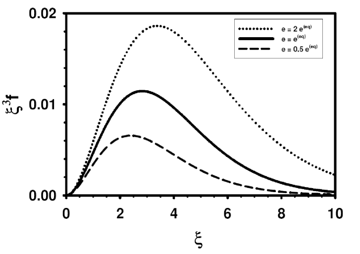
Figure 1: Function $f\xi^{3}$ for $p=0$ as a function of $\xi=\hbar ck/k_{B}T$ (in analogy to the spectral power density) obtained from the entropy maximization method applied to a grey body. $e=e^{(eq)}$ (solid, Planck function), $e=2e^{(eq)}$ (dotted), and $e=0.5e^{(eq)}$ (dashed). Larger energy implies a considerably higher photon occupation number and only a weak shift to larger wave numbers.

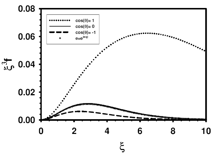
Figure 2: Function $f\xi^{3}$ as function of $\xi=\hbar ck/k_{B}T$ and for different values of the cosine of the angle $\Theta$ between $\vec{k}$ and $\vec{p}$. The value $\cos(\Theta)=1$ corresponds to photons parallel to $\vec{p}$, while $\cos(\Theta)=-1$ corresponds to anti-parallel photons. Here, the energy is roughly equipartitioned between ballistic and diffusive motion, i.e., $e=2e^{(eq)}$, $p=e^{(eq)}/c$; symbols indicate the equilibrium distribution.

We have numerically calculated $f$ for grey matter. In Fig. 1 a plot of $\xi^{3}f$ is shown as a function of $\xi=\hbar ck/k_{B}T$ for different values of $e$ at $p=0$. One observes that it is mainly the photon occupation number, which increases for higher energy $e$, while the shift of the wave number at maximum $f$ towards larger values is comparatively weak.
As the momentum $p$ increases, however the wave number is expected to be more affected. Figure 2 shows the distribution as a function of wave number for different values of the direction cosine. In this example, $pc=e^{(eq)}$ and $e=2e^{(eq)}$, which roughly means that half of the energy is thermal and half is ”ballistic”. The function $\xi^{3}f$ at $\cos(\Theta)=0$ is thus very close to the equilibrium distribution for $e=e^{(eq)}$, which is also plotted in the figure. Besides a change in their number density, the photons parallel ($\cos(\Theta)=1$) and anti-parallel ($\cos(\Theta)=-1$) to the beam are shifted towards higher and lower wave numbers, respectively.

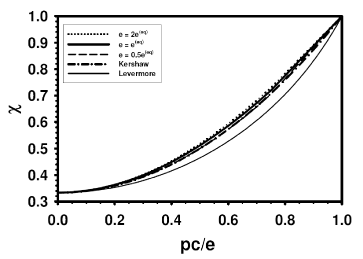
Figure 3: VEF of a grey body for the different cases listed in the legend. Deviations from $\chi_{K}$ are below the percentage range, deviations from the Levermore-Eddington factor $\chi_{ME}$ are larger.

The variable Eddington factor (VEF) obtained from our results turns out to be close to the heuristic proposal by Kershaw Kershaw1976 , $\chi_{K}=(1+2(cp/e)^{2})/3$. In particular, as required $\chi=1/3$ for $p=0$ and $\chi\rightarrow 1$ for $pc\rightarrow e$. Figure 3 shows a plot of $\chi$ as a function of $cp/e$ for various cases. $\chi_{K}$ seems to be a reasonable approximation for the VEF. For grey matter the integrals (27) and (28) can be calculated analytically by partial integration. Equation (34) implies then for the VEF near equilibrium (i.e., $e\approx e^{(eq)}$ and $pc\ll e$) $\chi(e,p)\approx(1+(3cp/2e)^{2})/3$.

The results obtained from the entropy production method are not only exact in the weak nonequilibrium limit, but provide the correct VEF in the limit of directed radiation ($p\to e/c$). This supports the conjecture that the entropy production method, in the present context, can serve as a useful approximation even far from equilibrium.

V.3 Non-grey matter

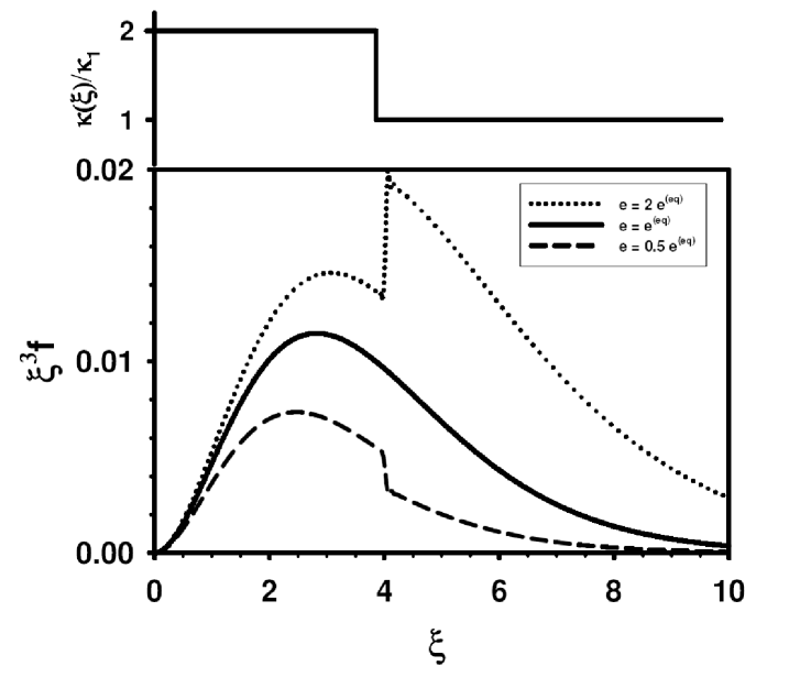
Figure 4: Top: Step-function absorption coefficient. Bottom: Function $f\xi^{3}$ for different $e/e^{(eq)}$-values. The change in $\kappa$ at $\xi=4$ implies a change in the distribution function. Higher $\kappa(k)$ values pulls the distribution function $f$ stronger towards the equilibrium distribution $f^{(eq)}$ because of stronger radiation-matter interaction.

As a simple example with mainly illustrative purpose, we consider now an artificial two-band absorption coefficient. We will use the non-dimensional quantity $\xi$ instead of the wave number $k$ and consider a step-function absorption-spectrum of the form $\kappa(\xi)=2\kappa_{1}$ for $\xi<\xi_{c}$ and $\kappa(\xi)=\kappa_{1}$ for $\xi>\xi_{c}$, where $\kappa_{1}$ is constant (cf. Fig. 4). This artificial spectrum $\kappa(\xi)$ describes matter-radiation interaction that is stronger for long than for short wavelengths. To be concrete, $\xi_{c}=4$, which gives $\kappa_{\rm Pl}=1.6\,\kappa_{1}$, $\kappa_{\rm Ro}=1.26\,\kappa_{1}$, and $\tilde{\kappa^{2}}/\tilde{\kappa}=1.89\,\kappa_{1}$.
One might have expected that for $e\to 0$ (emission limit) the value of $\kappa_{p}$ becomes equal to $\kappa(\xi\to 0)=2\kappa_{1}$, which is obviously not the case. The value $\kappa_{p}=1.89\,\kappa_{1}$ in this limit can be understood with the help of Eq. (35), which yields $f\approx f^{(eq)}\kappa(k)e/\tilde{\kappa}\hbar ck$. Hence $f$ is a given function of $k$ (or $\xi$), and is proportional to $e$. This implies that $\kappa_{p}$ is a fixed weighting of the spectral absorption coefficient.

The function $\xi^{3}f$ obtained from the minimum entropy production principle is shown in Fig. 4 for $p=0$ and different $e/e^{(eq)}$ values. A similar qualitative dependence of the photon occupation number on $e/e^{(eq)}$ appears as for grey matter. Furthermore, the step in $\kappa(\xi)$ leads to a step in $f$, such that the nonequilibrium distributions are closer to equilibrium for $\xi<\xi_{c}$. This pull of the long-wavelength part towards equilibrium can be understood from the larger $\kappa(\xi)$ value in this region. Indeed, stronger interaction of radiation with matter leads to stronger equilibration.

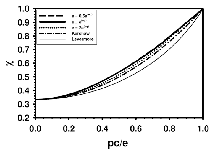
Figure 5: Same as in Fig. 3, but now for the step-function absorption coefficient of Fig. 4. The deviations from $\chi_{K}$ are a few percent, while deviations from $\chi_{ME}$ are twice as large.

The VEF for this special case of a stepwise absorption spectrum is shown in Fig. 5. The VEF has increased as compared to the grey medium, hence the deviations from Kershaw’s VEF are a little bit larger. The increase of $\chi$ at fixed $cp/e$ might be understood qualitatively as follows, if one interprets $\chi$ as a measure for the radiation pressure in direction of momentum $\vec{p}$. Because the considered absorption spectrum leads to enhanced equilibration of the long wavelength photons, there must be an increased amount of short wavelength photons contributing to the momentum $\vec{p}$, which leads to the larger $\chi$

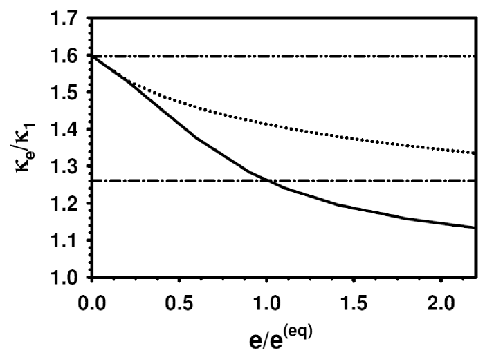
Figure 6: Effective absorption coefficient $\kappa_{e}$ (divided by $\kappa_{1}$) at $p=0$ for the step function absorption coefficient of Fig. 4. $\kappa_{e}$ obviously takes the Planck mean value (dashed-double-dotted) at $e=0$ (emission limit) and the Rosseland mean (dashed-dotted) at $e=e^{(eq)}$ (equilibrium radiation). For large energies, $\kappa_{e}$ will converge to $\kappa_{1}$, i.e. to the $\kappa(k)$ value at large wave numbers populated by most of the photons. Entropy maximization leads to a mean absorption $\kappa_{\rm ME}$ (dotted) with the correct Planck mean at $e=0$, but with a deviation from the Rosseland mean at $e=e^{(eq)}$.

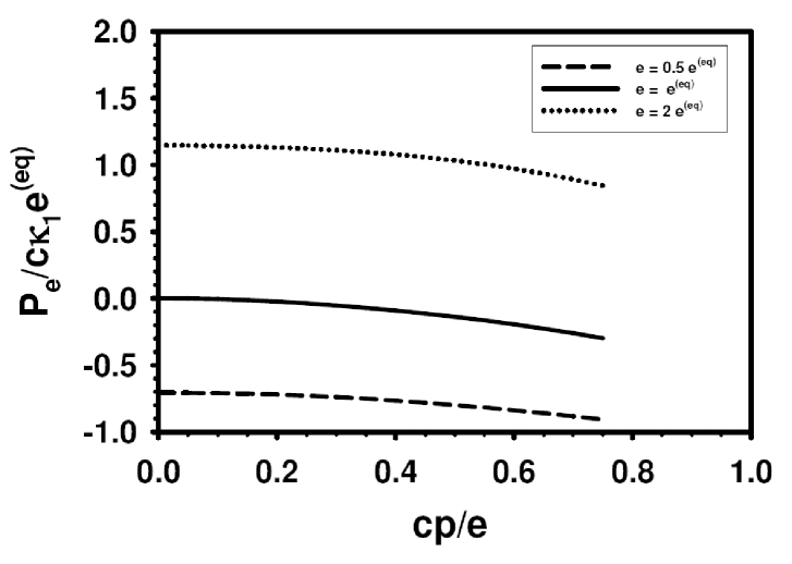
Figure 7: Energy loss function $P_{e}$ as a function of $cp/e$ for different $e/e^{(eq)}$ values. This figure illustrates that the zero of $P_{e}(e)$ is located at $e^{(eq)}$ only for equilibrium conditions, i.e., $p=0$. For finite $p$ the zero slightly shifts, i.e. $P_{e}(e^{(eq)})$ is finite.

The normalized effective absorption coefficient $\kappa_{e}/\kappa_{1}$ is shown in Fig. 6 as a function of $e/e^{(eq)}$ at $p=0$. In the limits $e\to 0$ and $e=e^{(eq)}$, the Planck and Rosseland mean are obtained as one expects. For $e\to\infty$ it holds $\kappa_{e}(e,p=0)\to\kappa_{1}$, as most photons will populate the short wavelength band. For finite $p$, it is inconvenient to discuss $\kappa_{e}(e,p)$ because the zero of $P_{e}(e,p)$ is no longer given by $e=e^{(eq)}$ but shifts as a function of $p$. (Note that finite $p$ is always associated with nonequilibrium.) An effective $\kappa_{e}$, however, can still be defined as in Eq. (9), but has a pole at $e^{(eq)}$ and a zero shifted away from $e^{(eq)}$. This fact is illustrated in Fig. 7, which shows that $P_{e}(e,p)$ starts to deviate from the value at $p=0$ as $p$ increases (particularly the shift of $P_{e}(e^{(eq)},p)$ from zero). Although equivalent, it might be more convenient to work with $P_{e}$ or with representations as in, e.g., Ref. Ripoll2008 than with $\kappa_{e}$, if general simulations of a fully coupled hydrodynamic radiation problem are performed.

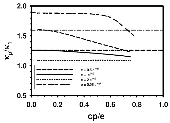
Figure 8: Effective absorption coefficient $\kappa_{p}$ (divided by $\kappa_{1}$) as a function of $cp/e$ for the step function absorption coefficient of Fig. 4. The dashed-dotted and the dashed-double-dotted lines indicate the Rosseland and Planck means, respectively.

Figure 8 shows the effective absorption coefficient $\kappa_{p}(e,p)/\kappa_{1}$ as a function of $pc/e$ for different $e/e^{(eq)}$-values. Again, for small $p$, $\kappa_{p}$ is large at small $e$ (emission approximation, where it goes to the value $1.89$), while near equilibrium the Rosseland mean is reproduced. At large $e$, $\kappa_{p}$ goes to $\kappa_{1}$ because the distribution function $f$ extends to higher and higher wave numbers. The same behavior occurs when $cp/e$ becomes large, i.e., $\kappa_{p}$ approaches $\kappa_{1}$, as can be concluded from the dotted curve in Fig. 2, which indicates that the distribution function of directed photons involves large wave numbers.

VI Comparison with the Maximum Entropy Method

In this section we compare our method with the well-known ME approach, where the radiation entropy is maximized. Especially, effective absorption coefficients and VEF are compared for the different explicit cases treated in the previous sections. The basic drawback of ME is the explicit independence of $f$ on $\kappa(k)$. The implicit dependence on $\kappa$ via radiation-matter coupling at the hydrodynamic level (i.e.,via an $e$ and $p$-dependence due to the ME constraints) is not able to spectrally resolve the absorption properties in the distribution function. Indeed, one can easily calculate $f$, which is given by StruchtrupUP

$$f_{\rm ME}=\frac{y}{\exp{(\hbar ck(\lambda_{e}-\vec{\lambda}_{p}\vec{s}))}-1}$$ (38)

with $e$ and $p$ dependent Lagrange parameters. At this level, information about the absorption spectrum is not contained.
On the other hand, according to Eq. (23), the distribution function $f$ obtained from entropy production minimization does explicitely depend on $\kappa(k)$. In subsection V.3, it has been shown that there is a significant and easily understandable effect of wave number dependent $\kappa(k)$ on the distribution function, and thus also on the effective absorption coefficients and on the VEF.
First, we note that because of the $\kappa$-independece of $f_{\rm ME}$, the associated VEF is a unique function of $e$ and $p$,

$$\chi_{\rm ME}=\frac{5}{3}-\frac{4}{3}\sqrt{1-\frac{3}{4}\frac{c^{2}p^{2}}{e^{2}}}\;\;,$$ (39)

which is the well-known Levermore-Eddington factor StruchtrupUP . It is also plotted in Figs. 3 and 5 for comparison. For grey matter the Eddington factors obtained by our approach and by ME are different, but probably similar enough to justify the use of $\chi_{\rm ME}$. For non-grey matter the deviations increase.
The difference in the effective absorption coefficients $\kappa_{e,p}$ is more important. In the limit case of weak nonequilibrium, where entropy production minimization reproduces the correct Rosseland mean, ME gives (i.e., up to leading order in $f_{\rm ME}-f^{(eq)}$)

$$\kappa_{\rm ME}=\frac{\int d^{3}k\,\kappa\,k^{2}\partial_{k}f^{(eq)}}{\int d^{3}k\,k^{2}\partial_{k}f^{(eq)}}\;\;,$$ (40)

which is clearly different from the correct Rosseland mean (18) (cf. StruchtrupUP ). Note that the two methods yield different results for the transport quantities in equilibrium limit, because the deviation from equilibrium, $\delta f=f-f^{(eq)}$, is different. Although the zero’th order term $f^{(eq)}$ is the same and $\delta f$ goes to zero, it is $\delta f$ which determines the transport coefficients. As an example, we have added the curve for $\kappa_{\rm ME}$ in Fig. 6. While the Planck limit ($e\to 0$) is correctly obtained by ME, there is a difference of about $10\%$ to the Rosseland limit ($e=e^{eq}$) for our simple example. As has been shown in Ref. StruchtrupUP , the ME approach is able to reproduce the Rosseland mean only if one considers a larger number of moments, which goes beyond a two-moment photo-hydrodynamic description of the photon gas with variables $e$ and $\vec{p}$.

A remark on the $\kappa$-dependence of our approach is in order. One might conclude from Eq. (21) that in the case of vanishing $\kappa$ the minimum entropy production rate approach is not defined, while the maximum entropy approach is defined because $\kappa$ does not appear. However, zero $\kappa$ means absence of equilibration. But maximum entropy requires that equilibration to the associated maximum entropy state already occurred. Because for zero $\kappa$ there is no process that drives the photon gas towards the associated maximum entropy state, both approaches encounter a similar conceptual problem.

VII Conclusion

The description of radiative heat transfer with photo-hydrodynamic equations requires a closure procedure to restrict the number of coupled equations. If radiative energy density $e$ and momentum density $\vec{p}$ are to be considered, effective absorption coefficients and a variable Eddington factor (VEF) have to be determined as a function of $e$ and $\vec{p}$. Using the minimization of the (local) entropy production rate of radiation and matter, a closure procedure is introduced that yields the photon distribution function, which depends on the spectral absorption coefficient, and which allows for the calculation of transport coefficients in general.
It has been shown that the derived expressions are exact near equilibrium, in the emission limit, and correctly describe directed radiation with a VEF $\chi=1$. Whereas the first fact is not very surprising as minimum entropy production is known to be exact near equilibrium, the other correct limiting behavior demonstrates that entropy production optimization can provide sound and useful results also far from equilibrium.
For the general case, effective absorption coefficients and a variable Eddington factor are found, which reasonably interpolate between the limiting cases, notably without introduction of any fit parameter. The variable Eddington factor for grey matter is close to the one proposed by Kershaw Kershaw1976 , and not far from the Levermore-Eddington factor, which can be derived from a maximum entropy approach.
In contrast to our approach, the distribution function obtained from the maximum entropy (ME) method does not contain the absorption spectrum. Hence, ME cannot describe frequency resolved absorption effects on the distribution function. An example of such an effect, which is taken into account by our method, is the enhanced photon equilibration in wave number bands with larger absorption as discussed in Sect. V.3. Another difference is that in the two-moment photo-hydrodynamic framework, ME is unable to reproduce the Rosseland mean absorption coefficient in the equilibrium limit.
Roughly speaking, the maximum entropy approach is a zero order approximation in the sense that radiation has equilibrated to a conditional maximum entropy state. Our approach can be understood as a first order approximation by assuming that the radiation is away from equilibrium and equilibrates according the minimum entropy production method. To summarize, we conjecture that this method may serve as a useful approach in various radiation heat transfer problems.
A benchmarking and critical discussion of specific application examples will be necessary in the future. Furthermore, the feasibility of improvements in the framework of multiband extensions Ripoll2008 or by taking into account higher order moments should be investigated.

References

- (1) Tien C L, ”Radiation properties of gases”, in Advances in heat transfer, Vol.5, Academic Press, New York (1968).
- (2) Jones G R and Fang M T C, Rep. Prog. Phys. 43, 1415 (1980).
- (3) Eby S D, Trepanier J Y, and Zhang X D, J. Phys. D: Appl Phys. 31, 1578 (1998).
- (4) Nordborg H and Iordanidis A A, J. Phys. D: Appl Phys. 41, 135205 (2008).
- (5) Goupil M J, Astron. Astrophys. 139, 353 (1984).
- (6) Levermore C D, J. Quant. Spectrosc. Radiat. Transfer. 31, 149 (1984).
- (7) Ripoll J-F and Wray A A, J. Comput. Phys. 227, 2212 (2008).
- (8) Siegel R and Howell J R, Thermal radiation heat transfer, Hemisphere Publishing Corp., Washington, Philadelphia, London (1992).
- (9) Ripoll J-F, Dubroca B and Duffa G, Combust. Theory Modeling 5, 261 (2001).
- (10) Ripoll J-F, J. Quant. Spectrosc. Radiat. Transfer. 83, 493 (2004).
- (11) Sampson D H, J. Quant. Spectrosc. Radiat. Transfer. 5, 211 (1965).
- (12) Kershaw D, ”Flux limiting nature’s own way”, Lawrence Livermore Laboratory, UCRL-78378 (1976).
- (13) Patch R W, J. Quant. Spectrosc. Radiat. Transfer. 7, 611 (1967).
- (14) Anile A, Pennisi S and Sammartino M, J. Math. Phys. 32, 544 (1991).
- (15) Minerbo G, J. Quant. Spectrosc. Radiat. Transfer. 20, 541 (1978).
- (16) Struchtrup H, in ”Rational extended thermodynamics” by I. Müller and T. Ruggeri, Springer, New. York, Second Edition, p. 308 (1998).
- (17) Planck M, Vorlesungen über die Theorie der Wärmestrahlung, Chapt. 5, Verlag J. A. Barth, Leipzig (1906).
- (18) Martyushev L M and Seleznev V D, Phys. Rep. 426, 1 (2006).
- (19) Christen T, J. Phys. D: Appl Phys. 39, 4497 (2006).
- (20) Oxenius J, J. Quant. Spectrosc. Radiat. Transfer. 6, 65 (1966).
- (21) Kröll W, J. Quant. Spectrosc. Radiat. Transfer. 7, 715 (1967).
- (22) Ford I J and Lee T-J 2001 J. Phys. D: Appl. Phys. 34, 413.
- (23) Christen T, J. Phys. D: Appl Phys. 40, 5719 (2007).
- (24) Landau L D and Lifshitz E M, Statistical Physics, Elsevier, Amsterdam (2005).
- (25) Essex C, The Astrophys. J. 285, 279 (1984).
- (26) Würfel P and Ruppel W, J. Phys. C: Solid State Phys. 18, 2987 (1985).
- (27) Kabelac S, ”Thermodynamik der Strahlung” Vieweg, Braunschweig (1994).
- (28) Santillan M, Ares de Parga G, and Angulo-Brown F, Eur. J. Phys. 19, 361 (1998).
- (29) Struchtrup H, Annals of Physics 266, 1 (1998).
- (30) Struchtrup H and Weiss W, Phys. Rev. Lett. 80, 5048 (1998).
- (31) Su B, J. Quant. Spectrosc. Radiat. Transfer. 64, 409 (2000).