Comment on “Phase Reduction of Stochastic Limit Cycle Oscillators”

In a recent Letter, Yoshimura and Arai Yoshimura claimed that the conventional phase stochastic differential equation (SDE) used in TN ; GP ; ER does not give a proper approximation to limit-cycle oscillators driven by noise, and proposed a modified phase SDE. Here we argue that their claim is not always correct; both SDEs are valid depending on the situation.

Since physical noise has an associated time scale and all oscillators have a characteristic rate of attraction, which of the two SDEs is appropriate depends on the relative sizes of these two scales. As a simple example, let us consider the Stuart-Landau (SL) model used in Yoshimura ; TN driven by a colored noise generated by the Ornstein-Uhlenbeck process (OUP) SP , which is rescaled such that the amplitude relaxation time explicitly appears while keeping the limit cycle and its isochrons invariant,

$$\dot{W}(t)=\{T^{-1}(1+ic)+i\omega\}W-T^{-1}(1+ic)|W|^{2}W+\sqrt{2\varepsilon}\xi(t),$$ (1)

where $W$ is a complex variable representing the oscillator state, $T$ is the relaxation time of the amplitude, $c$ and $\omega$ are parameters, $\varepsilon$ is the noise intensity, and $\xi(t)$ is OUP noise that is applied only to the real component of $W$ for simplicity. $\xi(t)$ is Gaussian-distributed, and its correlation function is given by $\langle\xi(t)\xi(s)\rangle=\exp\left(-|t-s|/\tau\right)/(2\tau)$, which converges to $\delta(t)$ as $\tau\to 0$. Thus, $\xi(t)$ gives a colored-noise approximation to the Wiener process SP .

Introducing the amplitude $R=|W|$ and the isochron phase $\phi=\arg W-c\ln|W|$ Yoshimura ; TN , Eq. (1) can be written as

$$\dot{R}(t)=T^{-1}(R-R^{3})+\sqrt{2\varepsilon}\cos(\phi+c\ln R)\ \xi(t),$$ (2)

$$\dot{\phi}(t)=\omega-\sqrt{2\varepsilon}R^{-1}\left\{\sin(\phi+c\ln R)+c\cos(\phi+c\ln R)\right\}\ \xi(t).$$ (3)

It is now clear that $T$ actually determines the relaxation time of the amplitude $R$. The limit cycle in the absence of the noise ($\varepsilon=0$) is simply $R(t)\equiv 1$ and $\phi(t)=\omega t+\mbox{const}$.

Two different SDEs have been previously derived describing this and other noisy oscillators. The non-agreement is due to the order in which the white-noise limit and the phase limit are taken Brown . The “conventional” model obtained by taking the phase limit in the first has the form:

$$d\phi(t)=\left[\omega+\varepsilon Z(\phi)Z^{\prime}(\phi)\right]dt+\sqrt{2\varepsilon}Z(\phi)dw(t),$$ (4)

where the phase sensitivity (or response) function $Z(\phi)=-\sin\phi-c\cos\phi$ in the present example. Yoshimura and Arai’s modified phase model obtained by taking the white-noise limit first is given by

$$d\phi(t)=\left[\omega+\varepsilon\left\{Z(\phi)Z^{\prime}(\phi)+Y(\phi)\right\}\right]dt+\sqrt{2\varepsilon}Z(\phi)dw(t),$$ (5)

where the extra term $Y(\phi)=(1+c^{2})\sin(2\phi)/2$ Yoshimura .

To see which of the two reduced phase SDEs (4, 5) approximates the original noisy SL model Eqs. (2, 3) better, we compare the stationary phase probability density functions (PDFs) obtained by direct Langevin simulations of Eqs. (2, 3) for different pairs of $(\tau,T)$ with the PDFs obtained from the two phase SDEs (4, 5) by numerically solving the corresponding Fokker-Planck equations. We fix $\omega=1$, $c=2$, $\varepsilon=0.01$, and vary $\tau$ and $T$ keeping $\tau T=0.001$ constant.

Figure 1(a) shows the stationary phase PDFs obtained for two typical cases, $T=0.01\ll\tau=0.1$ and $\tau=0.01\ll T=0.1$. The conventional phase SDE (4) nicely fits the original model when $T\ll\tau$, whereas the modified phase SDE (5) is better when $\tau\ll T$. Figure 1(b) shows mean-square errors of the approximate PDFs yielded by SDEs (4, 5) from the original PDF given by Eqs. (2, 3) as functions of $T(=0.001/\tau)$. It is clear that the conventional phase SDE (4) gives a better approximation for $T<T{*}$, while the modified SDE (5) is better for $T>T{*}$.

Summarizing, we have demonstrated that the conventional phase SDE (4) is also a proper approximation to noisy limit cycles with sufficiently fast amplitude relaxation, which can be used as a starting point for further analysis. It is a natural generalization of the ordinary phase equation driven by smooth signals (which becomes evident when written in the Stratonovich Langevin form SP ), and it has a practical advantage of being completely determined by $\omega$ and $Z(\phi)$, which are both experimentally measurable. The results in Yoshimura are valid when literally white noise is given to limit-cycle oscillators from the outset. However, white noise is actually an idealization of physical processes with small but finite time correlations. One should be careful of competing small time scales involved in the problem when the white-noise limit is taken. For example, near the bifurcation of a limit cycle, the attraction to the limit cycle is slow so that the SDE (5) is reasonable. However, far from the bifurcation or for relaxation oscillators where the time scale $T$ is very small, the conventional SDE (4) should be used.

Finally, the above intuitive arguments can be made rigorous by using a multi-scale or projection-operator method Brown ; SP , which yields a family of effective phase SDEs depending on the ratio $\tau/T$ TE . It can be shown that the two SDEs (4, 5) are actually two extreme cases corresponding to $T\to 0,\tau>0$ and $T>0,\tau\to 0$, respectively.

H. N. thanks Yoshiki Kuramoto and Kensuke Arai for useful comments.

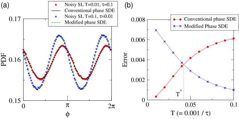
Figure 1: (a) Comparison of stationary phase PDFs obtained directly from Eqs. (2, 3) with those obtained from the phase SDEs (4, 5) for $(T,\tau)=(0.1,0.01)$ and $(0.01,0.1)$. (b) Mean-square errors of the approximate phase PDFs of SDEs (4, 5) from the original PDFs of Eqs. (2, 3) plotted as functions of the amplitude relaxation time $T(=0.001/\tau)$.

References

- (1) K. Yoshimura and K. Arai, Phys. Rev. Lett. 101, 154101 (2008).
- (2) J. Teramae and D. Tanaka, Phys. Rev. Lett. 93, 204103 (2004); H. Nakao, K. Arai, and Y. Kawamura, Phys. Rev. Lett. 98, 184101 (2007).
- (3) D. S. Goldobin and A. Pikovsky, Physica 351A, 126 (2005).
- (4) G. B. Ermentrout, R. F. Galán, and N. N. Urban, Phys. Rev. Lett. 99, 248103 (2007).
- (5) W. Horsthemke and R. Lefever, “Noise-Induced Transitions” (Springer, Berlin, 1984).
- (6) A similar situation arises in the analysis of classical Brownian particles with inertia driven by colored noises. See e.g. R. Kupferman, G. A. Pavliotis, and A. M. Stuart, Phys. Rev. E 70, 036120 (2004).
- (7) J. Teramae, H. Nakao, and G. B. Ermentrout, in preparation.