Reconnectionless CME eruption: putting the Aly-Sturrock conjecture to rest

Abstract

We demonstrate that magnetic reconnection is not necessary to initiate fast CMEs. The Aly-Sturrock conjecture states that the magnetic energy of a given force free boundary field is maximized when the field is open. This is problematic for CME initiation because it leaves little or no magnetic energy to drive the eruption, unless reconnection is present to allow some of the field to escape without opening. Thus, it has been thought that reconnection must be present to initiate CMEs. This theory has not been subject to rigorous numerical testing because conventional MHD numerical models contain numerical diffusion, which introduces uncontrolled numerical reconnection. We use a quasi-Lagrangian simulation technique to run the first controlled experiments of CME initiation in the complete lack of reconnection. We find that a flux rope confined by an arcade, when twisted beyond a critical amount, can escape to an open state, allowing some of the surrounding arcade to shrink and releasing magnetic energy from the global field. This mechanism includes a true ideal MHD instability. We conclude that reconnection is not a necessary trigger for fast CME eruptions.

1 Introduction

Coronal mass ejections (CMEs), are large expulsions of magnetic field and plasma from the solar corona. The kinetic and gravitational potential energy contained in a CME is around $10^{31-32}$ ergs, making these events some of the most energetic in our solar system (Canfield et al., 1980; Forbes, 2000; Hundhausen et al., 1994; Low, 1990, 2001). It is thought that CMEs derive their energy from the magnetic field of the solar corona because this field is the only possible source for such a large reserve of energy (e.g. Forbes, 2000; Klimchuk, 2001; Low, 1996).

The flux rope model is one possible pre-eruptive CME configuration. A flux rope is a length of magnetic field that has been twisted along its axis, often held in place in the corona by an overlying arcade or ambient field. It is thought that cool photospheric plasma can become be trapped in the center of a flux rope, creating a solar filament or prominence (van Ballegooijen and Martens, 1989; Ridgway et al., 1991; Priest et al., 1989). The flux rope configuration easily explains the clear three-part structure seen in many CMEs, specifically those associated with prominence eruptions (Hudson et al., 1999). Because these structures are present in the low corona where magnetic field is strong and plasma density is low, they are magnetic-field-dominated. Recently, movies from Hinode have shown interesting dynamics that are not described by the flux rope model which imply that at least some prominences are not low-$\beta$ (Berger et al., 2008), but the flux rope model remains useful. The lower coronal environment is also frequently modeled as being force-free because flow speeds are low, and $\mathbf{J}\times\mathbf{B}$ is the dominant force in the equation of motion. Gravity is also frequently ignored because it is a factor of $\sim 5$ weaker than the magnetic forces. Low-$\beta$ flux ropes are stable when the outward magnetic pressure force is balanced by an inward-directed tension force. In models, an exterior arcade field is often added to increase the tension force and keep the flux rope from simply expanding in length and width as twist is added. The approximate energy per unit length along the axis, $U$, stored in an unconfined Gold-Hoyle flux rope (Gold and Hoyle, 1960) is given by

$$U=\frac{1}{8\pi^{2}}\frac{\Phi^{2}b^{2}}{ln\left(1+b^{2}R^{2}\right)}$$ (1)

where $\Phi$ is the magnetic flux, $R$ is the radius of the tube, and $b$ is the twist parameter such that $\frac{B_{\phi}}{B_{z}}=br$ (Sturrock et al., 2001). As the twist accumulates, $b$ increases, $\Phi$ is constant and $R$ remains approximately constant so the total energy increases. When an unconfined flux rope anchored at both ends on the photosphere accumulates twist, its equilibrium state is expanded in length relative to the untwisted state so the twist per unit length does not necessarily increase with the total twist. Thus, flux ropes that are confined by an overlying arcade contain more energy because their length changes very little as $b$ increases.

The energy stored in the magnetic field is given by the volume integral of $B^{2}/8\pi$, up to conversion factors. The minimum energy of a magnetic system with a given photospheric boundary occurs in the potential, or vacuum field, configuration. As the field is stressed away from this configuration due to photospheric movements, the energy is increased above the evolving potential state by an amount commonly referred to as the magnetic ‘free energy’. If the field reverts to the potential configuration, this free energy is released and in the case of solar active regions, is available to drive a CME. If the reconnection is localized and helicity is conserved, the lowest accessible energy state may not be potential, so the free energy is an upper boundary on the amount of energy that can be released. There is a global cap on the amount of energy that the magnetic field can provide. The magnetic virial theorem asserts that the total pressure force can not exceed the tension force in a stable plasma environment (Priest, 1982). The related Aly-Sturrock conjecture states that the global magnetic energy of a force free field is at a maximum when the field is completely ‘open’. This refers to magnetic flux that is anchored at the solar surface and extends radially outward a significant distance so that, near the Sun, the field appears open (Aly, 1984, 1991; Sturrock, 1991). Many CME observations show prominences lifting off of the surface of the Sun, expanding to several solar radii and leaving behind long radial field lines. If this conjecture is correct, then the implication is that CMEs which open large amounts of field must derive the bulk of their kinetic energy from sources other than the magnetic field because the field energy is actually greater in the post-CME configuration. Order of magnitude analysis has shown, however, than the magnetic field is the only source of energy that can potentially drive a $10^{32}$erg CME (Forbes, 2000). This poses a significant problem to ideal CME models. In an azimuthally symmetric 2.5-D case, all of the field lines originally above a prominence-like feature would have to open to release the filament (Fig. 1a). Thus, in the 2.5-D case, to have an eruption which results in a net decrease of magnetic energy, reconnection must be present. There have been studies in which a 2.5-D field is shown to have magnetic energy exceeding the open field energy when mass loading is present, but it has not been demonstrated that these fields can erupt without reconnection (Low, 1996; Fong et al., 2002; Zhang and Low, 2004). In three dimensions, the flux rope is anchored in the photosphere, and the surrounding field can move away in the direction parallel to the flux rope axis (Fig. 1b). Reconnection is not necessary in the fully three-dimensional case, as not all of the field must be open to have an eruption, only the flux rope opens, and thus the eruption is not relevant to the hypothesis of Aly and Sturrock because some of the field remains closed (Low, 1986).

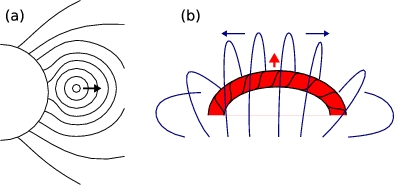
Figure 1: Behavior of flux rope expansion in 2.5D (a) and 3D (b).

The full Aly-Sturrock conjecture has yet to be disproved. However, it is not usually relevant to 3-dimensional models and analysis for the reasons stated above. A more relevant question which has been asked, is whether a configuration with some open force free field can contain less energy than a configuration with the same boundary conditions that is fully closed (Low, 1990). This question has been addressed semi-analytically by Wolfson and Low (1992) and Wolfson (1993), who showed that a fully closed field can contain magnetic free energy above the partially open field threshold, but they did not demonstrate a release mechanism for this energy. A demonstration of the ideal evolution of a field whereby free energy is stored then released, resulting in a partially open state, would once and for all eliminate the problem posed by the magnetic virial theorem and the Aly-Sturrock conjecture in a fully 3D case.

Sturrock et al. (2001) describe the possibility of driving CMEs with metastable magnetic fields. They analytically describe one system in particular as a known metastable state: the previously mentioned twisted flux rope under an overlying arcade. This system is metastable because it is stable (due to the confining arcade) against small perturbations, but the energy of the erupted flux rope is lower than the contained flux rope. If the rope is tightly wound, it can open and escape the arcade by herniating through it, leaving the deflated arcade near the footpoints. The amount of twist needed is not unreasonable for the solar surface. Analytically, for a flux rope that is ten times longer than its radius, the rope need only exceed 1.5 total turns about its axis to be in this metastable state (Sturrock, 1991).

Numerous simulations exist which model flux rope CME initiation of the metastable configuration described above (e.g. Aulanier et al., 2005; Fan and Gibson, 2004; Titov and Démoulin, 1999; Török et al., 2004; Roussev et al., 2003). Most of these simulations have found that it is possible to herniate through the arcade, but they do not agree exactly on how much twist is needed, or how unstable the resulting configuration is after the onset of writhe (helical geometry in the central field line) in the flux rope. Typically, these codes agree that the the critical twist needed to erupt is around 1.5 turns, and that it is possible to get an eruptive event by twisting the footpoints of a flux rope.

CME initiation with these flux ropes has been modeled both with and without reconnection as the intended primary destabilizing factor. Theories that do not involve reconnection are referred to as ideal “loss of equilibrium” models (e.g. Roussev et al., 2003). The initial structure generally undergoes an ideal instability, such as the MHD kink instability, caused by a large amount of twist. Another possibility, if mass loading is critical in keeping the structure contained, is that mass displacement could upset the force balance and start the CME (Klimchuk, 2001; Fong et al., 2002; Zhang and Low, 2004). Other theories, such as tether cutting (Moore and Roumeliotis, 1980) or “breakout” (Antiochos et al., 1999), explicitly include reconnection to decrease the strength of the overlying arcade. In models such as tether cutting and breakout, there are generally two stages of reconnection. Slow – Sweet-Parker style (Parker, 1963) – reconnection occurs early in the evolution and destabilizes the system, allowing it to expand. This is often followed by fast – Petcheck style (Petschek, 1964) – reconnection, which releases large amounts of energy in a short time and is believed to be the primary driver for fast, impulsive CMEs.

Essentially all existing numerical simulations of CME onset use Eulerian methods, in which a 3-D grid of values is used. With magnetic fields (and indeed all vector fields and flows), sharp gradients are not conserved because derivatives are represented as finite differences. For magnetic fields, this means that the field will reconnect if gradients approach the size of the grid whether the modeler wishes it or not. Techniques such as adaptive mesh refinement can reduce the rate of numerical reconnection, but can not remove it altogether. Hence it is not possible to separate the effects of ideal MHD evolution and magnetic reconnection with an Eulerian grid code. This can be problematic insofar as the reconnection destabilizes a metastable system. By switching to a Lagrangian (field-aligned) formulation, we eliminate all reconnection, allowing study of ideal MHD instabilities (DeForest and Kankelborg, 2007).

With our model, we are able to analyze simplified systems where topology is locked in and reconnection is not present. Note that we do not hypothesize that reconnection is not present in the Sun, only that to have a controlled numerical experiment, the effect of reconnection must be isolated, and we do this by eliminating it. Our method is unique in this way, and may offer insights that grid simulations can not. In particular, we are able to demonstrate the existence of a true MHD instability that can release free energy into a CME, even with no triggering reconnection.

2 Numerical Model

2.1 Computational Model

The code used in this work is called FLUX (FieldLine Universal relaXer) (DeForest and Kankelborg, 2007). This quasi-Lagrangian code represents a three-dimensional field as a collection of fluxons, or field lines with finite magnetic flux. Each fluxon is broken into piecewise linear segments called fluxels, which are joined at vertex points (Fig. 2). To reconnect, a fluxon must be explicitly broken and connected to another fluxon. With no reconnection, the code preserves magnetic topology; this is the case used in the current work. FLUX is coordinate free, so in order to compare the simulations with the Sun, we assume that our system is originally the size of an active region, which is a few tens of Mm across (1 spatial unit = 25 Mm). FLUX is under development and the version we used for this work is not a full magnetohydrodynamic code. It does not include the effects of mass or plasma; thus it does not model dynamics. We are neglecting short time-scale changes of the system in favor of concentrating on the large scale evolution.

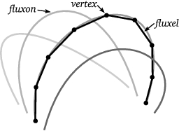
Figure 2: Geometry and nomenclature of the FLUX code. Finite-magnetic-flux field lines are called fluxons, which are broken into linear fluxel segments joined by vertices.

FLUX computes nonlinear force-free equilibrium solutions from a prescribed initial topology and connectivity by balancing the components of the Lorentz force, which are resolved as a magnetic pressure and a magnetic tension force:

$$0=-\nabla\left(\frac{B^{2}}{8\pi}\right)+\frac{\left(\mathbf{B}\cdot\nabla\right)\mathbf{B}}{4\pi}$$ (2)

The tension force is computed from the geometry of the other fluxels on the same fluxon (e.g. the angle between successive fluxels), and the pressure is computed based on the geometry of the nearest surrounding neighboring fluxels. Each vertex is moved in the direction of net calculated force until the ratio of the net force to the sum of the magnitudes of the forces on each vertex is below a threshold level. Once all vertices are below this threshold, e.g. $0.1\%$, the field is deemed to be in equilibrium. (A more detailed mathematical description is available in DeForest and Kankelborg (2007)).

Initial conditions in the code consist of a planar line-tied photosphere-like boundary with a set connectivity. The footpoint of each fluxon can be moved independently to simulate photospheric motions. After each footpoint movement, the field is allowed to relax to equilibrium before the next movement occurs. In this way, it is possible to create a quasi-static evolution of equilibrium states. The simulation is bounded at the top by an open hemisphere. Fluxons that intersect this surface are free to move around on it. Closed loops that approach the surface are truncated and become two separate fluxons that then move independently. Open fluxons move to equalize magnetic pressure (there is no curvature on the final fluxel), which has the effect that the magnetic field at the upper boundary is normal to the surface.

2.2 Simulation set up

The simulated systems consist of a flux rope, an overlying arcade, and an outer ring of open field lines. Figure 3(a) shows this set-up. The fluxons are tied to a planar lower boundary and evolve with a prescribed surface motion. The central flux rope is twisted incrementally in a solid body rotation pattern by four degrees each step and allowed to relax to equilibrium.The flux rope footpoints are set at 2 spatial units apart, or 50 Mm.

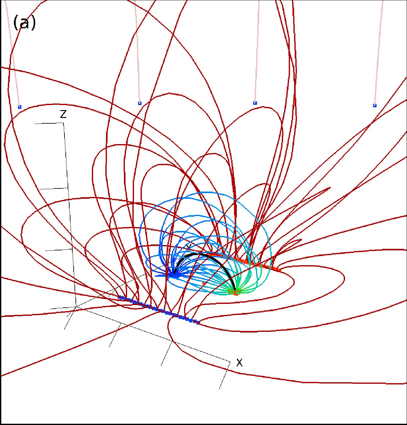
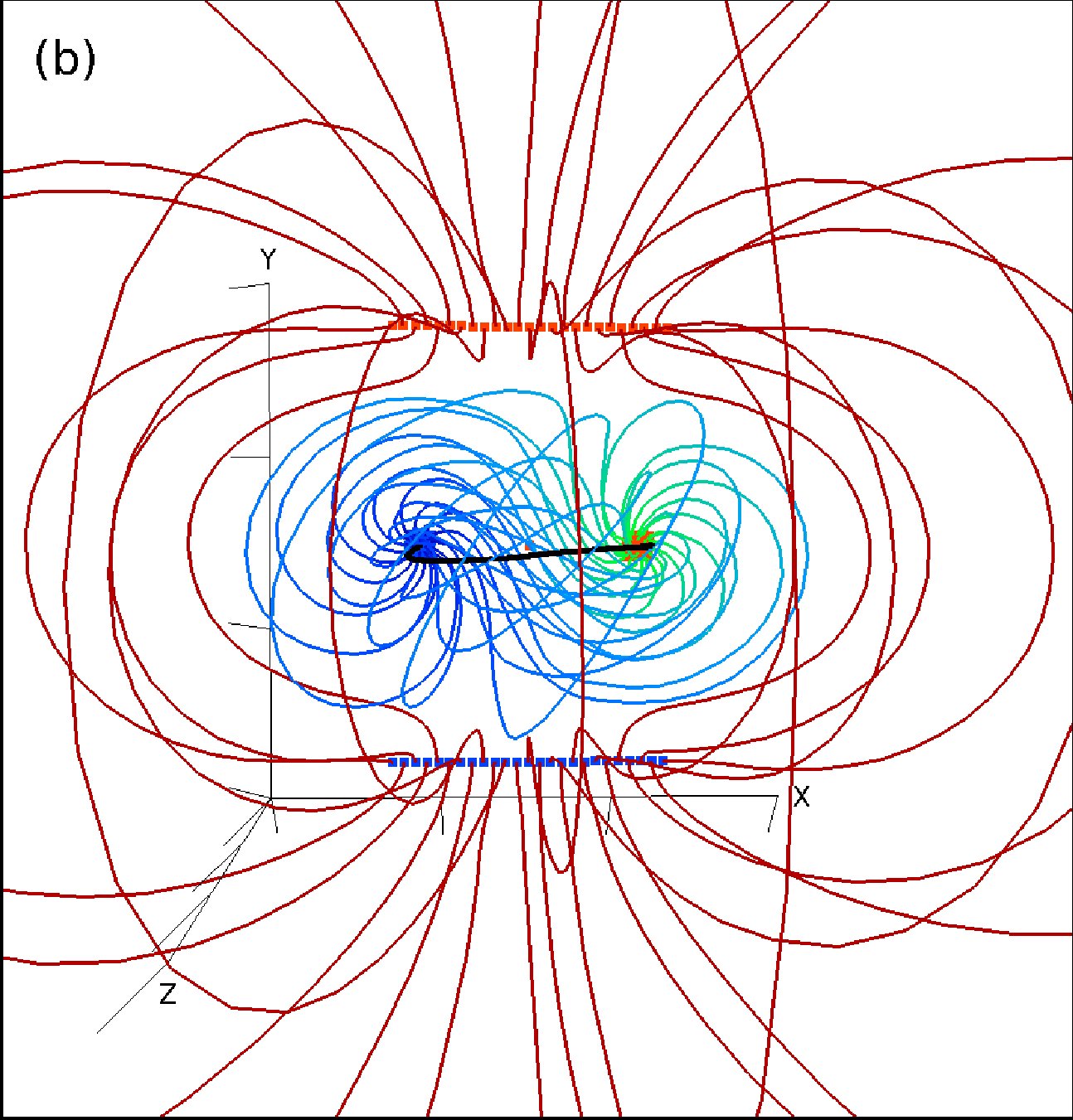
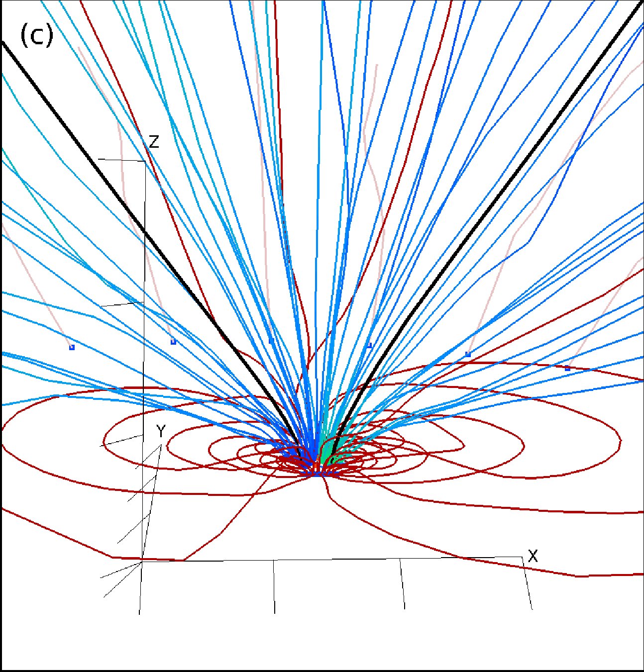
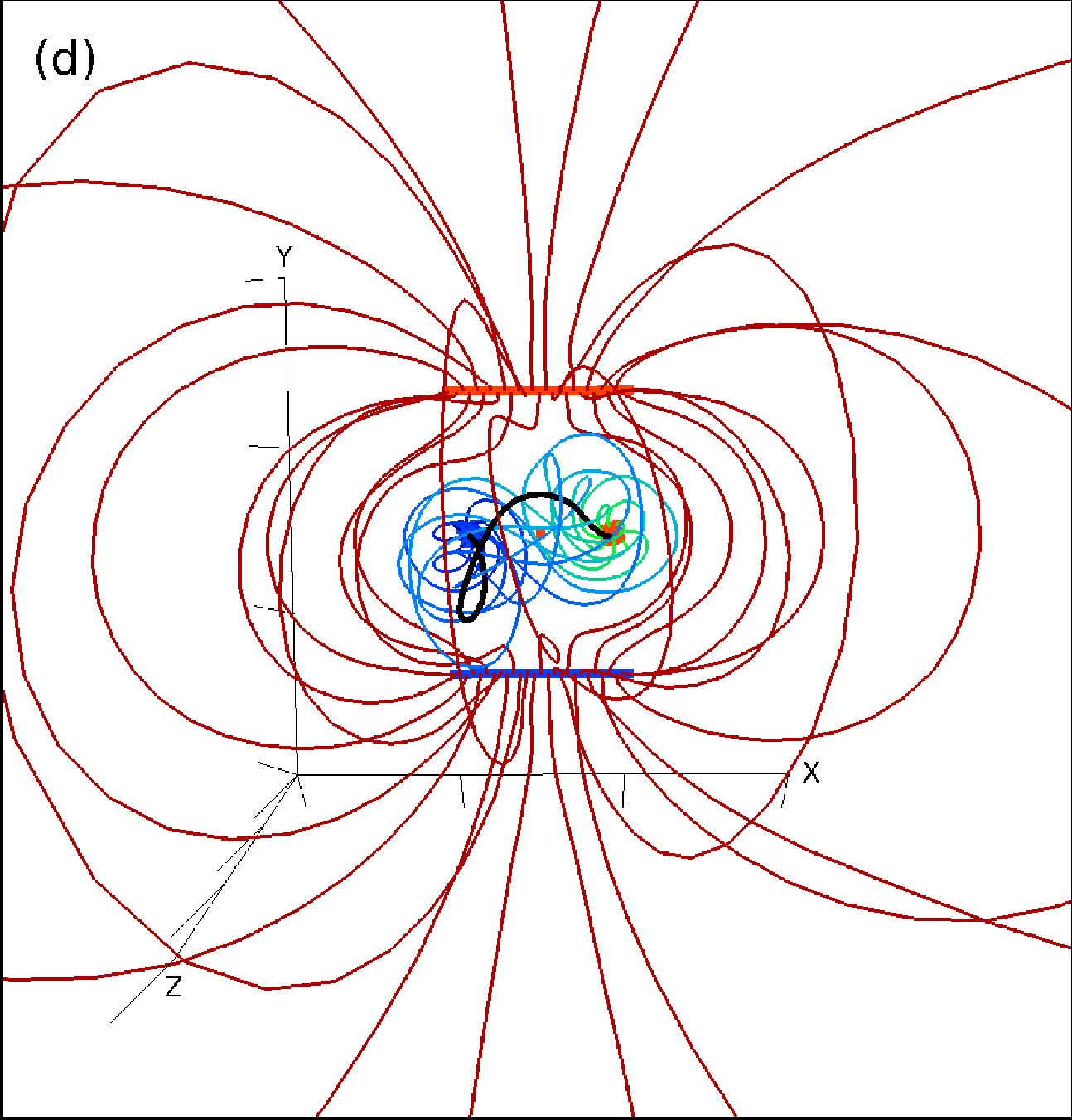
Figure 3: (a)-(c) Initial simulation set-up and evolution of a system with 75 fluxons where the arcade is 25 fluxons shown in red and the flux rope is 25 fluxons in shown in a gradient from blue to green to show directionality. The central fluxon is in black to highlight the flux rope axis. The outer ring of 25 fluxons is shown in light red. (a) The equilibrium system with no twist, (b) with 1 turn, which has not kinked, (c) with 1.43 turns which has herniated and is open at the upper boundary. (d) Shows a different system with 9 fluxons in the flux rope and 3 units of flux (27 fluxons) in the arcade at 2.1 turns, which demonstrates kinking without herniation. Note that the systems with one unit of arcade flux do exhibit a slight kink while confined as evidenced by a small distortion in the central fluxon, but the systems with higher arcade flux exhibit much stronger kink before herniation.

One difficulty in examining these results has been with the energy calculation. Our code calculates the energy of every fluxel based on the cross sectional area it occupies and its length. In regions where the fluxons are close to each other, this method works extremely well, but it has more trouble for the outer-most fluxons in a system. We call this the ‘last-fluxon’ problem and it is discussed by DeForest and Kankelborg (2007). The volume that the last fluxon occupies is infinite, so it cannot be treated as small, violating the approximation used by the code. Once the system has herniated and expanded fully, the number of last-fluxons is much greater, exaggerating the difficulty in determining the post-eruption energy. The open hemispherical surface at $35\,R_{\odot}$ and an outer ring of fluxons were added to alleviate this problem. As a consequence of the surface, the field opens once it encounters the hemisphere and expands to fill the volume.

The footpoints of the outer ring remain stationary throughout the simulation. This outer ring is present to minimize the ‘last fluxon problem’ because with the ring, none of the arcade or flux rope fluxons will be a last fluxon. The ring is positioned far from the rope and the arcade, about $2\,R_{\odot}$ away, so it does not effect the evolution. The outer boundary at a radius of $35\,R_{\odot}$ is much farther than the physical regime of applicability of FLUX. The transition to solar wind occurs at $\sim 4\,R_{\odot}$(Parker, 1960; Kohl et al., 1997), so at most, our results have physical meaning up to this height.

We performed several simulations with varying numbers of fluxons in the flux rope and the arcade, each with the same basic set-up. The flux rope consists of 9, 16, 25, 36 or 49 fluxons arranged in a square on the photosphere. The footprint of the flux rope is the same size in each case. For the rest of this paper, a unit of magnetic flux refers to the amount of magnetic flux associated with the flux rope, or the number of fluxons in the flux rope. In these simulations, the flux rope and the ring consist of one unit of flux, and the arcade contains one, two, or three units.

3 Simulation Results

In all cases, we find that the flux rope herniates through the arcade after a certain amount of twist has been applied, entraining a few arcade fluxons with it as it goes. Figure 3(a)-(c) demonstrates a typical sequence of events for a case of a 25 fluxon flux rope and a one-unit magnetic flux arcade. First, the flux rope twists about its central axis under the arcade. After about 1.4 turns have been applied to the flux rope (for one unit of arcade flux), the rope herniates. In this case, the flux rope does not significantly kink – the central axis remains mostly un-twisted – but in the case of a stronger arcade, the flux rope does kink before it herniates. The stronger the arcade, the flatter the flux rope is, and the more twist is required to initiate herniation. Figure 3(d) shows the three-unit arcade system after it has undergone writhe; the black central fluxon is no longer straight. The onset of kink does not trigger the herniation through the arcade. The flux rope continues to twist and writhe until it begins to herniate. In every case, after the onset of herniation, the flux rope expands rapidly while the arcade deflates. Figure 4 shows a plot of height of the flux rope vs. twist imparted, for various fluxon densities with one unit of arcade flux. The expansion occurs extremely rapidly, within one equilibrium step, once the flux rope breaks through the arcade.

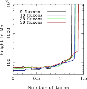
Figure 4: The flux rope remains well confined as it is twisted until it herniates rapidly through the arcade. The data shown are for systems with one unit of flux in the arcade.

We label this rapid expansion as an “eruption,” because the size of the flux rope increases by a factor of 100 or more and breaks through the open surface in a single equilibrium time step, while releasing a non-trivial amount of energy. Thus, these large expansions are deemed eruptions and the flux rope fluxons are labeled as open.

The amount of twist needed to herniate through a given arcade strength varies with the number of fluxons used to represent the field (Fig. 4; this may be indicative of grid effects that are setting an unstable twist level or seeding the instability. Because of the discrete nature of fluxons, the system is not always symmetric, and this probably accounts for some uncertainly in the critical twist. There is not always a consistent trend with fluxon density, and so there may be other reasons behind this behavior.

The energy of the final erupted state is less than the energy of the confined flux rope (Figure 5). Note that the presence of the open boundary does not skew these results. The magnetic energy that escapes through the boundary would not be available to drive the CME in any case because it is present beyond the transition to the solar wind. In the latter stages of the expansion, the twist per unit length in the flux rope is small, and hence the free energy is low. It is the initial expansion that drives the CME, not the later expansion. Compared to the physical case, we overestimate the final magnetic energy of the system because our boundary is much farther out than the transition. A significant amount of energy is available to drive a CME, even without reconnection.

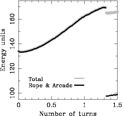
Figure 5: A typical energy plot for the simulations run. This one shows the energy evolution of a 25 fluxon flux rope with a one unit flux arcade. As the flux rope is twisted under the arcade, the energy increases steadily. Once the system herniates, the energy loss is substantial. Note that the energy in the flux rope and arcade only (black line) drops to lower than the initial level. This is because most of the energy in the system at that point is in the outer ring fluxons which are highly stressed toward the horizontal.

This simulation allows us to put a strong upper and lower bound on the amount of energy that is released with the eruption. Of the free energy injected, $12.5\%$ is lost after herniation. The energy calculated in the ring field after herniation is an overestimate, and the energy in the flux rope and the arcade is an underestimate for the following reasons. The ring field was added so that all of the last fluxons were that ring. As stated earlier, we do not trust the energy calculation for the ring field, especially considering that before herniation less than $1\%$ of the system’s energy was in the ring field compared to $\sim 40\%$ after herniation. Also, on a spherical solar surface, the ring field would be farther away than the disk limb if the flux rope were at disk-center, and consequently would not be highly sheared away from radial after the eruption, so it would not store much more energy than it had initially.

Because of the unreliability of the final energy in the ring field, we also looked at the energy in only the flux rope and the arcade. In this partial system, the final energy is less than the initial potential energy in part because some of the energy is carried through the open boundary and lost from the calculation, and in part because this limited system does not account for any background solar field that may be deformed by the CME.

Despite these effects, we are able to conclude that a significant amount of energy is released and could be used to drive an impulsive CME. The best way to resolve the energy would be to run a similar system as a full-Sun simulation in spherical geometry so that there are no last-fluxons, and include an estimate of the energy outside the upper boundary with a force free field extrapolation. This future work may be able to determine quantitatively how much magnetic energy available; a figure which is highly dependent on the geometry of each event.

4 Discussion

Our simulations show that reconnection is not necessary to initiate a CME and that impulsive CMEs may be possible without explosive reconnection. This theory is not new; it was originally published by Sturrock et al. (2001), who describe the existence of metastable states, specifically a system similar to the one we have studied. Since then, other solar physicists have studied this system computationally (Fan and Gibson, 2004; Török et al., 2004; Aulanier et al., 2005, etc.). The results from these studies show that a highly twisted flux rope can herniate through a confining magnetic arcade and reconnect into a plasmoid, causing an eruption. However, this is the first study of this system in the complete lack of reconnection. In general, our results agree with those of other research groups.

The fact that many of these simulations, including ours, agree that about 1.5 total turns is needed to herniate through an arcade implies that reconnection is not greatly important to the overall stability of the system. If it were, then we would expect our ideal simulation to support significantly more twist and therefore release more energy than the dissipative simulations. The exact value of the critical twist will depend on the configurations of the system: strength of the arcade, width of the flux rope, the twist profile within the flux rope, etc. But even with these variables, we conclude that highly twisted flux ropes can not easily be confined by external field, even when the reconnection rate is extremely small.

Current research on the twist available photospheric fields indicates that there may be an excess of one full turn available in many active regions (Leka et al., 2005). This implies that many pre-eruptive active regions may be on the brink of an ideal instability when they flare or erupt, regardless of the eventual trigger mechanism.

Our results together with the results of Wolfson and Low (1992) and Wolfson (1993) can finally put to rest the concerns that the Aly-Sturrock conjecture have created over the initiation of CMEs. Although it has not been proven that a closed force free field can have more energy than a fully open one, that question is not relevant in the complex three dimensional system that is our Sun. A more appropriate question is whether a closed force free field can contain more energy than a configuration with some open field given the same lower boundary and connectivity. Wolfson and Low (1992) began to answer that question with semi-analytic techniques and successfully showed that it was possible. We have proven that it is possible to transition between closed and partially open field while still releasing free energy without reconnection and without the need for gravitational or other non-magnetic confinement. At the beginning of the century there was, “still no model which demonstrates that a partly open magnetic field can be achieved solely by a loss of ideal MHD equilibrium or stability.” (Forbes, 2000). Happily, this statement is no longer true.

References

- Aly [1984] J. J. Aly. On some properties of force-free magnetic fields in infinite regions of space. ApJ, 283:349–362, August 1984. 10.1086/162313.
- Aly [1991] J. J. Aly. How much energy can be stored in a three-dimensional force-free magnetic field? ApJ, 375:L61–L64, July 1991. 10.1086/186088.
- Antiochos et al. [1999] S. K. Antiochos, C. R. DeVore, and J. A. Klimchuk. A Model for Solar Coronal Mass Ejections. ApJ, 510:485–493, January 1999. 10.1086/306563.
- Aulanier et al. [2005] G. Aulanier, P. Démoulin, and R. Grappin. Equilibrium and observational properties of line-tied twisted flux tubes. A&A, 430:1067–1087, February 2005. 10.1051/0004-6361:20041519.
- Berger et al. [2008] T. E. Berger, R. A. Shine, G. L. Slater, T. D. Tarbell, A. M. Title, T. J. Okamoto, K. Ichimoto, Y. Katsukawa, Y. Suematsu, S. Tsuneta, B. W. Lites, and T. Shimizu. Hinode SOT Observations of Solar Quiescent Prominence Dynamics. ApJ, 676:L89–L92, March 2008. 10.1086/587171.
- Canfield et al. [1980] R. C. Canfield, C.-C. Cheng, K. P. Dere, G. A. Dulk, D. J. McLean, E. J. Schmahl, R. D. Robinson, Jr., and S. A. Schoolman. Radiative energy output of the 5 September 1973 flare. In P. A. Sturrock, editor, Skylab Solar Workshop II, pages 451–469, 1980.
- DeForest and Kankelborg [2007] C. E. DeForest and C. C. Kankelborg. Fluxon modeling of low-beta plasmas. Journal of Atmospheric and Terrestrial Physics, 69:116–128, February 2007. 10.1016/j.jastp.2006.06.011.
- Fan and Gibson [2004] Y. Fan and S. E. Gibson. Numerical Simulations of Three-dimensional Coronal Magnetic Fields Resulting from the Emergence of Twisted Magnetic Flux Tubes. ApJ, 609:1123–1133, July 2004. 10.1086/421238.
- Fong et al. [2002] B. Fong, B. C. Low, and Y. Fan. Quiescent Solar Prominences and Magnetic-Energy Storage. ApJ, 571:987–998, 2002. 10.1086/340070.
- Forbes [2000] T. G. Forbes. A review on the genesis of coronal mass ejections. J. Geophys. Res., 105:23153–23166, October 2000. 10.1029/2000JA000005.
- Forbes and Isenberg [1991] T. G. Forbes and P. A. Isenberg. A catastrophe mechanism for coronal mass ejections. ApJ, 373:294–307, May 1991. 10.1086/170051.
- Gold and Hoyle [1960] T. Gold and F. Hoyle. On the origin of solar flares. MNRAS, 120:89–+, 1960.
- Hudson et al. [1999] H. S. Hudson, L. W. Acton, K. L. Harvey, and D. E. McKenzie. A Stable Filament Cavity with a Hot Core. ApJ, 513:L83–L86, March 1999. 10.1086/311892.
- Hundhausen et al. [1994] A. J. Hundhausen, A. L. Stanger, and S. A. Serbicki. Mass and energy contents of coronal mass ejections: SMM results from 1980 and 1984-1988. In J. J. Hunt, editor, Solar Dynamic Phenomena and Solar Wind Consequences, the Third SOHO Workshop, volume 373 of ESA Special Publication, pages 409–+, December 1994.
- Klimchuk [2001] J. A. Klimchuk. Theory of coronal mass ejections. AGU Geophysical Monograph, 125, 2001.
- Kohl et al. [1997] J. L. Kohl, G. Noci, E. Antonucci, G. Tondello, M. C. E. Huber, L. D. Gardner, P. Nicolosi, L. Strachan, S. Fineschi, J. C. Raymond, M. Romoli, D. Spadaro, A. Panasyuk, O. H. W. Siegmund, C. Benna, A. Ciaravella, S. R. Cranmer, S. Giordano, M. Karovska, R. Martin, J. Michels, A. Modigliani, G. Naletto, C. Pernechele, G. Poletto, and P. L. Smith. First Results from the SOHO Ultraviolet Coronagraph Spectrometer. Sol. Phys., 175:613–644, October 1997. 10.1023/A:1004903206467.
- Leka et al. [2005] K. D. Leka, Y. Fan, and G. Barnes. On the Availability of Sufficient Twist in Solar Active Regions to Trigger the Kink Instability. ApJ, 626:1091–1095, June 2005. 10.1086/430203.
- Low [1986] B. C. Low. Blowup of force-free magnetic fields in the infinite region of space. ApJ, 307:205–212, August 1986. 10.1086/164407.
- Low [1990] B. C. Low. Equilibrium and dynamics of coronal magnetic fields. ARA&A, 28:491–524, 1990. 10.1146/annurev.aa.28.090190.002423.
- Low [2001] B. C. Low. Coronal mass ejections, magnetic flux ropes, and solar magnetism. J. Geophys. Res., 106:25141–25164, November 2001. 10.1029/2000JA004015.
- Low [1996] B. C. Low. Solar Activity and the Corona. Sol. Phys., 167:217–265, August 1996.
- Moore and Roumeliotis [1980] R. L. Moore and G. Roumeliotis. Triggering of Eruptive Flares - Destabilization of the Preflare Magnetic Field Configuration. In Z. Svestka and B. V. Jackson and M. E. Machado, editors, IAU Colloq. 133: Eruptive Solar Flares, pages 69+-, 1992.
- Parker [1960] E. N. Parker. The Hydrodynamic Treatment of the Expanding Solar Corona. ApJ, 132:175–+, July 1960.
- Parker [1963] E. N. Parker. The Solar-Flare Phenomenon and the Theory of Reconnection and Annihiliation of Magnetic Fields. ApJS, 8:177–+, July 1963.
- Petschek [1964] H. E. Petschek. Magnetic Field Annihilation. In W. N. Hess, editor, The Physics of Solar Flares, pages 425–+, 1964.
- Priest [1982] E. R. Priest. Solar Magnetohydrodynamics. D. Reidel Publishing Co., Dordrecht, 1982.
- Priest et al. [1989] E. R. Priest, A. W. Hood, and U. Anzer. A twisted flux-tube model for solar prominences. I - General properties. ApJ, 344:1010–1025, September 1989. 10.1086/167868.
- Ridgway et al. [1991] C. Ridgway, E. R. Priest, and T. Amari. A twisted flux tube model for solar prominences. III - Magnetic support. ApJ, 367:321–332, January 1991. 10.1086/169631.
- Roussev et al. [2003] I. I. Roussev, T. G. Forbes, T. I. Gombosi, I. V. Sokolov, D. L. DeZeeuw, and J. Birn. A Three-dimensional Flux Rope Model for Coronal Mass Ejections Based on a Loss of Equilibrium. ApJ, 588:L45–L48, May 2003. 10.1086/375442.
- Sturrock [1991] P. A. Sturrock. Maximum energy of semi-infinite magnetic field configurations. ApJ, 380:655–659, October 1991. 10.1086/170620.
- Sturrock et al. [2001] P. A. Sturrock, M. Weber, M. S. Wheatland, and R. Wolfson. Metastable Magnetic Configurations and Their Significance for Solar Eruptive Events. ApJ, 548:492–496, February 2001. 10.1086/318671.
- Titov and Démoulin [1999] V. S. Titov and P. Démoulin. Basic topology of twisted magnetic configurations in solar flares. A&A, 351:707–720, November 1999.
- Török et al. [2004] T. Török, B. Kliem, and V. S. Titov. Ideal kink instability of a magnetic loop equilibrium. A&A, 413:L27–L30, January 2004. 10.1051/0004-6361:20031691.
- van Ballegooijen and Martens [1989] A. A. van Ballegooijen and P. C. H. Martens. Formation and eruption of solar prominences. ApJ, 343:971–984, 1989. 10.1086/167766.
- Wolfson [1993] R. Wolfson. Energy Requirements for Opening the Solar Corona. ApJ, 419:382–+, December 1993. 10.1086/173491.
- Wolfson and Low [1992] R. Wolfson and B. C. Low. Energy buildup in sheared force-free magnetic fields. ApJ, 391:353–358, May 1992. 10.1086/171350.
- Zhang and Low [2004] M. Zhang and B. C. Low. Magnetic Energy Storage in the Two Hydromagnetic Types of Solar Prominences. ApJ, 600:1043–1051, 2004. 10.1086/379891.