Comparison of Binary Classification Based on Signed Distance Functions with Support Vector Machines

1  Introduction

Efficient and accurate computational solutions for binary classification problems are currently of interest in many contexts, particularly in biomedical informatics and computational biology where the interesting genomic and proteomic data sets are imbued with dimensional complexity and confounded by noise. Over the past several years it has been effectively demonstrated that binary classification of genomic and proteomic data can be used to connect a molecular snapshot of an individual’s internal state with the presence or absence of a disease. This potential promises to revolutionize personalized medicine and is fueling the development and analysis of robust classification algorithms. Among the existing classification algorithms Support Vector Machine (SVM) methods have distinguished themselves as efficient, accurate and robust. Applications of Radial Basis Function Networks (RBFN) to classification have also generated attention.

We consider only a geometric (rather than statistical) formulation of the binary classification problem. Namely, we suppose that the space of measurements $X$ is divided into two subsets, $A$ and its compliment $A^{c}=X\setminus A$. We are given data $\{x_{i}\}$ for which we know the membership in $A$ or $A^{c}$ of each data point. From this data the binary classification problem is to construct a rule or classifier that we can use to predict the class of new, uncharacterized data. As an example, the data may be measurements of genomic activation levels, one class might be measures from individuals known to have a certain type of disease while the other class may be from individuals without the disease.

The linear SVM method was originally designed to be geometric and robust through a constraint that it produce a dividing surface of maximal margin between data of opposite type. However, it has been shown that nonlinear SVM implementations actually are built around reconstruction of the indicator function that ties the location of the data to its class ([2]). The indicator function:

$$i_{A}(x)=\left\{\begin{array}[]{cl}1&\mbox{if $x\in A$}\\ -1&\mbox{if $x\in A^{c}$,}\end{array}\right.$$

encodes only the most primitive geometric information. In [2] we proposed an alternative tool for classification, the Signed Distance Function (SDF), that measures the signed distance from the data to the boundary between the classes, i.e.

$$b_{A}(x)=\left\{\begin{array}[]{cl}d(x,A^{c})&\mbox{if $x\in A$}\\ -d(x,A)&\mbox{if $x\in A^{c}$,}\end{array}\right.$$ (1)

where $d$ is a distance function. While the SDF has not previously been applied to classification, it has been an important tool in other fields, such as free boundary problems in fluid dynamics, and so has a rich mathematical development that could be exploited. We have tested rudimentary classification algorithms based on the idea of reconstructing the SDF from training data. We note that this reconstruction could be based on any accepted method of regression, including SVM or RBFN regression. Thus, new SVM or RBFN classification methods could be built on the SDF foundation. One simple, yet appealing, choice for the nonlinear regression is the least squares regression discussed in [7]. We have implemented this approach in the algorithm for nonlinear data describe below.

We investigate the performance of a simple SDF based method by direct comparison with standard SVM packages, as well as K-nearest neighbor and RBFN methods. We present experimental results comparing the SDF approach with other classifiers on both synthetic geometric problems and five benchmark clinical microarray data sets. On both geometric problems and microarray data sets, the non-optimized SDF based classifiers perform just as well or slightly better than well-developed, standard SVM methods. These results demonstrate the potential accuracy of SDF-based methods on some types of problems.

Algorithms. A procedure for training an SDF classifier is given in Algorithm 1. It takes as arguments a training data set $\{(x_{i},y_{i})\}_{i=1}^{N}$ and a smoothing parameter $\gamma$, and returns a trained SDF classifier

$$\hat{B}(x)=\mbox{sign}[\hat{b}_{A}(x)]=\mbox{sign}[\sum_{i=1}^{N}\hat{\alpha}_{i}K(x,x_{i})].$$

In the SDF paradigm the input training data are marked as to class, but they do not come marked with the values $b_{A}(x_{i})$, and hence these need to be approximated. A reasonable and simple first approximation of $b_{A}$ at $\{x_{i}\}_{i=1}^{m}$ is given by

$$b_{i}=i_{A}(x_{i})\cdot\min_{j\neq i}\{d(x_{i},x_{j}):i_{A}(x_{j})\neq i_{A}(x_{i})\},$$ (2)

i.e. the signed projection onto the data of opposite type.

Algorithm 1
1. For each $1\leq k\leq d$, compute the Pearson’s correlation coefficient $w_{k}$ between $(y_{1},y_{2},...,y_{N})^{T}$ and $(x_{1k},x_{2k},...x_{Nk})$.
2. Calculate the weighted distance matrix $\mathbf{D}$, with $D_{ij}=\sqrt{\sum_{k=1}^{d}[w_{k}(x_{ik}-x_{jk})]^{2}}$ for any $1\leq i,j\leq N$.
3. Estimate the variance of the Gaussian kernel function, $\sigma$, by the Root Mean Squared Distance (RMSD) $\hat{\sigma}=\sqrt{\frac{2}{N(N+1)}\sum_{i=1}^{N-1}\sum_{j=i+1}^{N}D_{ij}^{2}}$.
4. Calculate the Gaussian kernel matrix $\mathbf{K}$, with $K_{ij}=K(x_{i},x_{j})=\exp(-D_{ij}^{2}/2\sigma^{2})$ for any $1\leq i,j\leq N$.
5. Estimate $\mathbf{b}=\{b_{i}\}_{i=1}^{N}$ at the training data $\{x_{i}\}_{i=1}^{N}$ using (2).
6. Reconstruct $b_{A}$, on the entire domain through regression, i.e. solving the linear system of equations $$(\mathbf{K}+N\gamma\mathbf{I})\mathbf{\alpha}=\mathbf{b}$$ (3) where $\mathbf{I}$ is the identity matrix.

In the preliminary explorations on microarray data, we used the Pearson’s correlation coefficients to rank the relevant importance of the features (Step 1), and use these to compute the weighted distances between cases (Step 2). The parameter $\sigma$ determines the width of the Gaussian functions centered at the data points. In Algorithm 1, $\sigma$ was determined based on mean data distances (Step 3). The Gaussian kernel matrix was calculated from the distance matrix just in the same way as in conventional SVM algorithms (Step 4). The SDF was estimated using the simple heuristic improvement of equation (2). The problem of solving (3) is well-posed since $(\mathbf{K}+N\gamma\mathbf{I})$ is strictly positive definite and the condition number will be good provided that $N\gamma$ is not too small (Step 6).

The procedure for training the SDF classifier on linearly separable data is simpler and can be obtained by removing Step 2 and 3 from Algorithm 1, and replacing the Gaussian kernel function $K(x_{i},x_{j})$ by the inner product operator $\langle x_{i},x_{j}\rangle=x_{i}^{T}x_{j}$.

2  Experimental Results

In [2] we investigated these methods in linearly separable problems, the 4 by 4 checkerboard problem and two cancer diagnosis problems involving micro-array data. In this manuscript we report tests of primitive SDF based methods on two new geometric problems and four additional cancer diagnosis problems. We compare our algorithm with the standard SVM methods, as well as the Lagrangian SVM [6] and Proximal SVM [3]. A software implementation of our algorithm with GUI can be found at: http://people.vanderbilt.edu/ minhui.xie/sdf2005/.

Checkerboard Problems. In [2] we presented numerical results on the 4 by 4 checkerboard problem, a geometric problem that is known to be hard. In those tests SDF based classification outperformed the best reported SVM results as well as standard SVM packages.

Here we perform a simple experiment that sheds light on the performance advantage of the SDF methods in this geometrical context. In this test we divide the square $X:=[-1,1]\times[-1,1]$ into two sets, $A:=[0,1]\times[0,1]$ and its complement. We choose a data set uniformly at random in $X$ and solve equation (3) setting the right hand side to: (a) the exact distances to the boundary $b$, (b) the exact values of the indicator function $I$. We then use the coefficients determined in each case to compute the value of the function $|B(0,0)|$, whose value is a direct measure of the error in fitting the boundary between the classes at the corner. We considered 100 independent trials and calculated the mean value of the absolute error and its variance (Table 1). The SDF average local error was an order of magnitude lower as was its standard deviation, and as the number of input data increases it decreases rapidly toward zero. This demonstrates the main advantage of the SDF over the indicator function: the SDF is much more suitable for the regression step.

Data Set	SDF Error	IF Error
100 points	$0.0365\pm.0268$	$0.5180\pm.2530$
500 points	$0.0135\pm.0104$	$0.4916\pm.1066$
1000 points	$0.0098\pm.0084$	$0.4775\pm.0996$

Table 1: A comparison of the local error and reliability of the SDF and indicator function (IF) regression applied to a local checkerboard problem.

Biased distribution of data. We observed in the linear tests that the SDF classification particularly outperformed the SVM methods on skewed data sets. We give here an explanation that illustrates a clear advantage of using the SDF over the indicator function. Suppose that the data has more samples of one type than the other. If the indicator function is approximated then the additional data of one type will reinforce that value of the indicator function effectively enlarging the region predicted in that set. If the signed distance function is approximated, the distance to the boundary is reinforced which does not move the boundary.

We illustrate this with a simple example. Consider the data set $\{(0,1),(.1,1),(-.1,1),(0,-1)\}$. The original SVM would place the separating line for this data at $y=0$. However, the Proximal SVM places it at $y=-.2$ and the Lagrangian SVM places it at $y=-.125$. If more points are added near (0,1), the separating line is pushed further into $y<0$. However, the SDF linear classifier places the separating line at $y=0$ up to an error comparable to machine epsilon.

Microarray Data Sets. In [2] we tested an SDF-based classifier on two standard genomic data sets involving cancer diagnosis from microarray experiments and found the SDF-based classification to do as well or better than standard LIBSVM routines. In the current paper we further compare the generalization performances of SDF-based classifier versus three other types of distance-based classifiers: KNN, Radial Basis Function Networks (RBFN) and SVM. We use the following microarray data sets:

• The Breast Cancer data set [11] consists of 49 tumor samples with 7129 human genes each. There are two different response variables in the data set: one describes the status of the estrogen receptor (ER), and the other one describes the status of the lymph nodal (LN). Of the 49 samples, 25 are ER+ and 24 are ER-, 25 are LN+ and 24 are LN-.

• The Colon Cancer data set [1] consists of 40 tumor and 22 normal colon tissues with 2000 genes each.

• The Leukemia data set [4] consists of 72 samples with 7129 genes each. Each patient represented by a sample has either acute lymphoblastic leukemia (ALL) or acute myeloid leukemia (AML). Of the 72 samples, 47 are ALL and 25 are AML.

We tested the four classifiers in 100 independent trials on each of the data sets. In each trial, the data set is divided randomly into a training set and a test set according to the ratio of 2:1. We use Gaussian kernel functions for RBFN, SVM and SDF. We claim that the classifiers are comparable in this setting since they are used under exactly the same conditions: (i) They share the same training set and test set in each trial, (ii) SVM and SDF share the same $\gamma=10^{-7}$, (iii) SVM and SDF used the same weighted kernel matrix in each trial, (iv) SVM and RBFN used the same $\sigma$, which is computed in each trial by the RMSD as described in Algorithm 1 in Section 3.4.

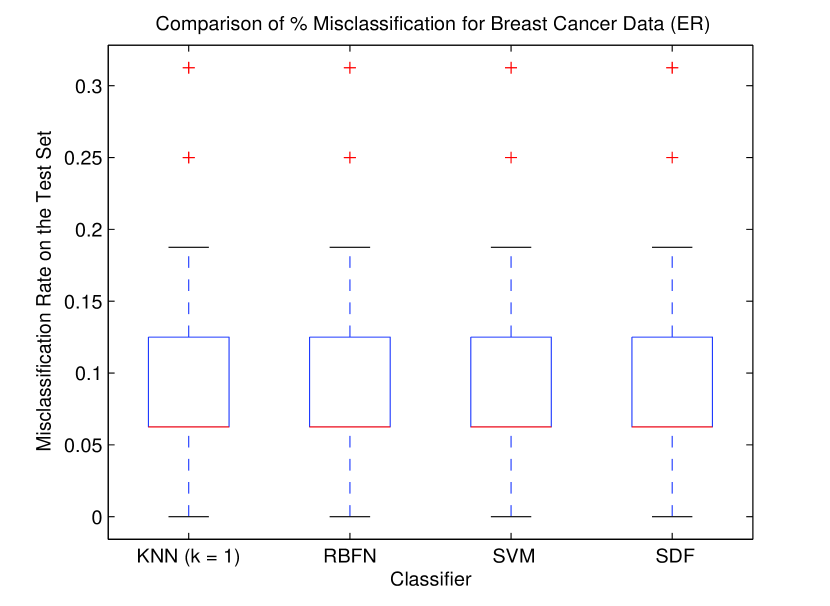
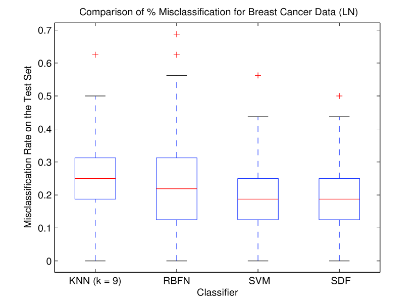
Figure 1: Comparison misclassification rates for breast cancer data.

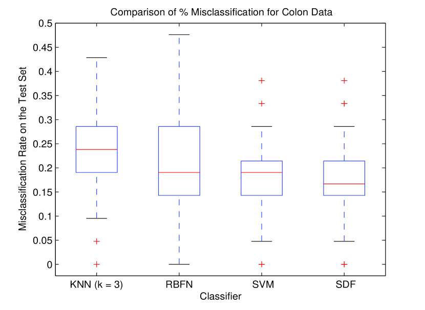
Figure 2: Comparison of misclassification rates for colon data.

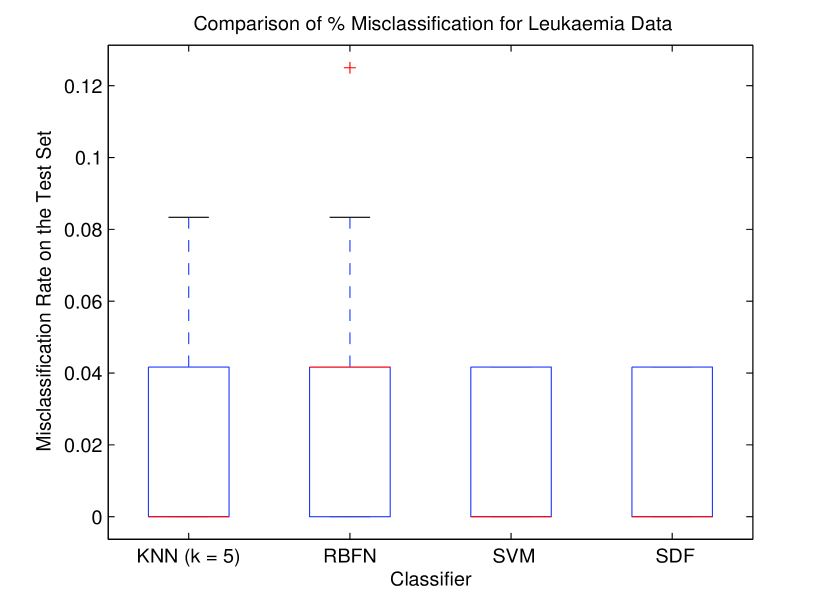
Figure 3: Comparison of misclassification rates for leukemia data.

Figures 1, 2, and 3 show the boxplots of the test error rates in 100 trials, on the breast cancer data set, the colon cancer data set, and the leukemia data set, respectively. In Figure 1 the response variable is ER and in Figure 1 the response variable is LN. Since the sample size of each data set is less than 80, KNN with a large number of neighbors might not achieve good performance due to overfitting. Hence in our experiments we test KNN only with $k$ from 1 to 10.

Data Set	KNN	RBFN	SVM	SDF
Breast (ER)	.0912	.0912	.0869	.0869
Breast (LN)	.2400	.2425	.2106	.2100
Colon	.2200	.2143	.1700	.1662
Leukemia	.0146	.0321	.0167	.0167

Table 2: Comparison of misclassification rates averaged over 100 trials on randomly divided data.

Table 1 shows the test error rates averaged over the 100 independent trials for each classifier. KNN with 1, 9, 3, 5, 5 neighbors achieves the best (in the averaging sense) generalization performance for the breast cancer data (ER), breast cancer data (LN), colon cancer data, colon cancer data with 5 samples removed, and the leukemia data, respectively. In the table we only keep the averaged test error rates for the best KNN.

From the boxplots and the averaged test error rates, we can see that the performances of KNN and RBFN on the microarray data sets are generally not as good as those of SVM and SDF. The performance of the SDF classifier matches that of the SVM method on the breast cancer data (ER) and the leukemia data, exceeds it on the breast cancer data (LN) and the colon cancer data.

3  Conclusions

From the experimental results shown above, SDF-based classifiers promise to be more accurate than current generation classification methods and just as efficient computationally. Because it is geometrical, SDF-based nonlinear classification is theoretically a more faithful and natural generalization of the original SVM concept than existing nonlinear SVM implementations. The algorithm presented in the paper and used in the experiments is the most naive version, so there are many other directions of future development that need to be followed. These might include investigation of different methods for initialization of $\{b_{i}\}_{i=1}^{m}$ from the training data, optimization of $b_{A}$ through various iteration schemes, exploration of the use of different regression techniques, such as the SVM and RBFN regression, to reconstruct $b_{A}$ from $\{b_{i}\}_{i=1}^{m}$, and so on. Due to the importance of biological data sets which usually have thousands of features, we would also try various dimension reduction techniques, such as Principal Component Analysis (PCA), Independent Component Analysis (ICA), and Factor Analysis to preprocess the data and analyze the interactions between dimensionality and performance of the SDF-based classifiers. Finally, as pointed out in [2] the use of the SDF in other applications and its relationship to deep mathematical results might be exploited to both improve implementations and provide rigorous validation of the process.

References

- [1] U. Alon, N. Barkai, D. Notterman, K. Gish, S. D. Ybarra, Mack, and A. Levine, Broad patterns of gene expression revealed by clustering analysis of tumor and normal colon tissues probed by oligonucleotide arrays, Proc. Natl. Acad. Sci, 96:6745–6750, 1999.
- [2] E.M. Boczko and T. Young, Signed distance functions: A new tool in binary classification, ArXiv preprint: CS.LG/0511105.
- [3] G. Fung and O.L. Mangasarian, Proximal support vector machine classifiers, preprint, 2001.
- [4] T. Golub, D. Slonim, P. Tomayo, C. Huard, M. Gaasenbeck, J. Mesirov, H. Coller, M. Loh, J. Downing, M. Caligiuri, C. Bloomfield, and E. Lander, Molecular classification of cancer: Class discovery and class prediction by gene expression monitoring, Science, 286:531–537, 1999.
- [5] L.P. Li, C. Weinberg, T. Darden, and L. Pedersen, Gene selection for sample classification based on gene expression data: Study of sensitivity to choice of parameters of the ga/knn method, Bioinformatics, 17:1131–1142, 2001.
- [6] O.L. Mangasarian and D. R. Musicant, Lagrangian support vector machines, J. Mach. Learn. Res., 1:161–177, 2001.
- [7] T. Poggio and S. Smale, The mathematics of learning: Dealing with data, Notices Amer. Math. Soc., 50:537–544, 2003.
- [8] M.A. Shipp, K.N. Ross, P. Tamayo, A.P. Weng, J.L. Kutok, R.C. Aguiar, M. Gaasenbeek, M. Angelo, M. Reich, G.S. Pinkus, T. Ray TS, M.A. Koval, K.W. Last, A. Norton, T.A. Lister, J. Mesirov, D.S. Neuberg, E.S. Lander, J.C. Aster, and T.R. Golub, Diffuse large b-cell lymphoma outcome prediction by gene-expression profiling and supervised machine learning, Nat. Med., 8:68–74, 2002.
- [9] D. Singh, P.G. Febbo, K. Ross, D.G. Jackson, J. Manola, C. Ladd, P. Tamayo, A.A. Renshaw, A.V. D’Amico, J.P. Richie, E.S. Lander, M. Loda, P.W. Kantoff, T.R. Golub, and W.R. Sellers, Gene expression correlates of clinical prostate cancer behavior, Cancer Cell, 1:203–9, 2002.
- [10] A. Statnikov, C.F. Aliferis, I. Tsamardinos, D. Hardin, and S. Levy, A comprehensive evaluation of multicategory classification methods for microarray gene expression cancer diagnosis, Bioinformatics, 21(5), 631-43, 2005.
- [11] M. West, C. Blanchette, H. Dressman, E. Huang, S. Ishida, R. Spang, H. Zuzang, J. John A. Olson, J.R. Marks, and J.R. Nevins, Predicting the clinical status of human breast cancer by using gene expression profiles, Proc. Natl. Acad. Sci., 98(20):11462–11467, September 2001.