Binary Classification Based on Potential Functions

Abstract – We introduce a simple and computationally trivial method for binary classification based on the evaluation of potential functions. We demonstrate that despite the conceptual and computational simplicity of the method its performance can match or exceed that of standard Support Vector Machine methods.

Keywords: Machine Learning, Microarray Data

1  Introduction

Binary classification is a fundamental focus in machine learning and informatics with many possible applications. For instance in biomedicine, the introduction of microarray and proteomics data has opened the door to connecting a molecular snapshot of an individual with the presence or absence of a disease. However, microarray data sets can contain tens to hundreds of thousands of observations and are well known to be noisy [2]. Despite this complexity, algorithms exist that are capable of producing very good performance [10, 11]. Most notable among these methods are the Support Vector Machine (SVM) methods. In this paper we introduce a simple and computationally trivial method for binary classification based on potential functions. This classifier, which we will call the potential method, is in a sense a generalization of the nearest neighbor methods and is also related to radial basis function networks (RBFN) [4], another method of current interest in machine learning. Further, the method can be viewed as one possible nonlinear version of Distance Weighted Discrimination (DWD), a recently proposed method whose linear version consists of choosing a decision plane by minimizing the sum of the inverse distances to the plane [8].

Suppose that $\{\mathbf{y}_{i}\}_{i=1}^{m}$ is a set of data of one type, that we will call positive and $\{\mathbf{z}_{i}\}_{i=1}^{n}$ is a data set of another type that we call negative. Suppose that both sets of data are vectors in ${{\mathbb{R}}}^{N}$. We will assume that ${{\mathbb{R}}}^{N}$ decomposes into two sets $Y$ and $Z$ such that each $\mathbf{y}_{i}\in Y$, $\mathbf{z}_{i}\in Z$ and any point in $Y$ should be classified as positive and any point in $Z$ should be classified as negative. Suppose that $\mathbf{x}\in{{\mathbb{R}}}^{N}$ and we wish to predict whether $\mathbf{x}$ belongs to $Y$ or $Z$ using only information from the finite sets of data $\{\mathbf{y}_{i}\}$ and $\{\mathbf{z}_{i}\}$. Given distance functions $d_{1}(\cdot,\cdot)$ and $d_{2}(\cdot,\cdot)$ and positive constants $\{a_{i}\}_{i=1}^{m}$, $\{b_{i}\}_{i=1}^{n}$, $\alpha$ and $\beta$ we define a potential function:

$$I(\mathbf{x})=\sum_{i=1}^{m}\frac{a_{i}}{d_{1}(\mathbf{x},\mathbf{y}_{i})^{\alpha}}-\sum_{i=1}^{n}\frac{b_{i}}{d_{2}(\mathbf{x},\mathbf{z}_{i})^{\beta}}.$$ (1)

If $I(\mathbf{x})>0$ then we say that $I$ classifies $\mathbf{x}$ as belonging to $Y$ and if $I(\mathbf{x})$ is negative then $\mathbf{x}$ is classified as part of $Z$. The set $I(\mathbf{x})=0$ we call the decision surface. Under optimal circumstances it should coincide with the boundary between $Y$ and $Z$.

Provided that $d_{1}$ and $d_{2}$ are sufficiently easy to evaluate, then evaluating $I(\mathbf{x})$ is computationally trivial. This fact could make it possible to use the training data to search for optimal choices of $\{a_{i}\}_{i=1}^{m}$, $\{b_{i}\}_{i=1}^{n}$, $\alpha$, $\beta$ and even the distance functions $d_{j}$. An obvious choice for $d_{1}$ and $d_{2}$ is the Euclidean distance. More generally, $d$ could be chosen as the distance defined by the $\ell^{p}$ norm, i.e. $d(\mathbf{x},\mathbf{y})=\|\mathbf{x}-\mathbf{y}\|_{p}$ where

$$\|\mathbf{x}\|_{p}\equiv\left(x_{1}^{p}+x_{2}^{p}+\ldots+x_{N}^{p}\right)^{1/p}.$$ (2)

A more elaborate choice for a distance $d$ might be the following. Let $\mathbf{c}=(c_{1},c_{2},\ldots,c_{N})$ be an $N$-vector and define $d_{\mathbf{c}}$ to be the $\mathbf{c}$-weighted distance:

$$d_{\mathbf{c},p}(\mathbf{x},\mathbf{y})\equiv\left(c_{1}|x_{1}-y_{1}|^{p}+c_{2}|x_{2}-y_{2}|^{p}\right.\\ +\ldots+\left.c_{N}|x_{N}-y_{N}|^{p}\right)^{1/p}.$$ (3)

This distance allows assignment of different weights to the various attributes. Many methods for choosing $\mathbf{c}$ might be suggested and we propose a few here. Let $\mathbf{C}$ be the vector associated with the classification of the data points, $C_{i}=\pm 1$ depending on the classification of the i-th data point. The vector $\mathbf{c}$ might consist of the absolute values univariate c orrelation coefficients associated with the $N$ variables with respect to $\mathbf{C}$. This would have the effect of emphasizing directions which should be emphasized, but very well might also suppress directions which are important for multi-variable effects. Choosing $\mathbf{c}$ to be $1$ minus the univariate $p$-values associated with each variable could be expected to have a similar effect. Alternatively, $\mathbf{c}$ might be derived from some multi-dimensional statistical methods. In our experiments it turns out that $1$ minus the $p$-values works quite well.

Rather than $a_{i}=b_{i}=1$ we might consider other weightings of training points. We would want to make the choice of $\mathbf{a}=(a_{1},a_{2},\ldots,a_{m})$ and $\mathbf{b}=(b_{1},b_{2},\ldots,b_{n})$ based on easily available information. An obvious choice is the set of distances to other test points. In the checkerboard experiment below we demonstrate that training points too close to the boundary between $Y$ and $Z$ have undue influence and cause irregularity in the decision curve. We would like to give less weight to these points by using the distance from the points to the boundary. However, since the boundary is not known, we use the distance to the closest point in the other set as an approximation. We show that this approach gives improvement in classification and in the smoothness of the decision surface.

Note that if $p=2$ in (2) our method limits onto the usual nearest neighbor method as $\alpha=\beta\rightarrow\infty$ since for large $\alpha$ the term with the smallest denominator will dominate the sum. For finite $\alpha$ our method gives greater weight to nearby points.

In the following we report on tests of the efficacy of the method using various $\ell^{p}$ norms as the distance, various choices of $\alpha=\beta$ and a few simple choices for $\mathbf{c}$, $\mathbf{a}$, and $\mathbf{b}$.

2  A Simple Test Model

We applied the method to the model problem of a 4 by 4 checkerboard. In this test we suppose that a square is partitioned into a 16 equal subsquares and suppose that points in alternate squares belong to two distinct types. Following [7], we used 1000 randomly selected points as the training set and 40,000 grid points as the test set. We choose to define both the distance functions by the usual $\ell^{p}$ norm. We will also require $\alpha=\beta$ and $a_{i}=b_{i}=1$ Thus we used as the potential function:

$$I(\mathbf{x})=\sum_{i=1}^{m}\frac{1}{\|\mathbf{x}-\mathbf{y}_{i}\|_{p}^{\alpha}}-\sum_{i=1}^{n}\frac{1}{\|\mathbf{x}-\mathbf{z}_{i}\|_{p}^{\alpha}}.$$ (4)

Using different values of $\alpha$ and $p$ we found the percentage of test points that are correctly classified by $I$. We repeated this experiment on 50 different training sets and tabulated the percentage of correct classifications as a function of $\alpha$ and $p$. The results are displayed in Figure 1. We find that the maximum occurs at approximately $p=1.5$ and $\alpha=4.5$.

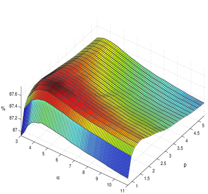
Figure 1: The percentage of correct classifications for the 4 by 4 checkerboard test problem as a function of the parameters $\alpha$ and $p$. The maximum occurs near $p=1.5$ and $\alpha=4.5$. Notice that the graph is fairly flat near the maximum.

The relative flatness near the maximum in Figure 1 indicates robustness of the method with respect to these parameters. We further observed that changing the training set affects the location of the maximum only slightly and the affect on the percentage correct is small.

Finally, we tried classification of the 4 by 4 checkerboard using the minimal distance to data of the opposite type in the coefficients for the training data, i.e. $\mathbf{a}$ and $\mathbf{b}$ in:

$$I(\mathbf{x})=\sum_{i=1}^{m}\frac{(1+\epsilon)a_{i}^{\beta}}{\|\mathbf{x}-\mathbf{y}_{i}\|_{p}^{\alpha}}-\sum_{i=1}^{n}\frac{(1-\epsilon)b_{i}^{\beta}}{\|\mathbf{x},\mathbf{z}_{i}\|_{p}^{\alpha}}.$$

With this we obtained $96.2\%$ accuracy in the classification and a noticably smoother decision surface (see Figure 2(b)). The optimized parameters for our method were $p\approx 3.5$ and $\alpha\approx 3.5$. In this optimization we also used the distance to opposite type to a power $\beta$ and the optimal value for $\beta$ was about $3.5$. In [7] a SVM method obtained $97\%$ correct classification, but only after 100,000 iterations.

Figure 2: (a) The classification of the 4 by 4 checkerboard without distance to boundary weights. In this test $95\%$ were correctly classified. (b) The classification using distance to boundary weights. Here $96.2\%$ were correctly classified.

3  Clinical Data Sets

Next we applied the method to micro-array data from two cancer study sets Prostate_Tumor and DLBCL [10, 11]. Based on our experience in the previous problem, we used the potential function:

$$I(\mathbf{x})=\sum_{i=1}^{m}\frac{(1+\epsilon)a_{i}^{\beta}}{d_{\mathbf{c},p}(\mathbf{x},\mathbf{y}_{i})^{\alpha}}-\sum_{i=1}^{n}\frac{(1-\epsilon)b_{i}^{\beta}}{d_{\mathbf{c},p}(\mathbf{x},\mathbf{z}_{i})^{\alpha}},$$ (5)

where $d_{\mathbf{c},p}$ is the metric defined in (3). The vector $c_{i}$ was taken to be $1$ minus the univariate p-value for each variable with respect to the classification. The weights $a_{i}$, $b_{i}$ were taken to be the distance from each data point to the nearest data point of the opposite type. Using the potential (5) we obtained leave-one-out cross validation (LOOCV) for various values of $p$, $\alpha$, $\beta$, and $\epsilon$. For these data sets LOOCV has been shown to be a valid methodology [10]

On the DLBCL data the nearly optimal performance of $98.7\%$ was acheived for many parameter combinations. The SVM methods studied in [10, 11] achieved $97.5\%$ correct on this data while the $k$-nearest neightbor correctly classified only $87\%$. Specifically, we found that for each $1.6\leq p\leq 2.4$ there were robust sets of parameter combinations that produced performance better than SVM. These parameter sets were contained generally in the intervals: $10<\alpha<15$ and $10<\beta<15$ and $0<\epsilon<.5$.

For the DLBCL data when we used the $\ell^{p}$ norm instead of the weighted distances and also dropped the data weights ($\epsilon=\beta=0$) the best performance sank to $94.8\%$ correct classification at $(p,\alpha)=(2,6)$. This illustrates the importance of these parameters.

For the Prostrate_tumor data set the results using potential (5) were not quite as good. The best performance, $89.2\%$ correct, occured for $1.2\leq p\leq 1.6$ with $\alpha\in[11.5,15$, $\beta\in[12,14]$, $\epsilon\in[.1,.175]$ . In [10, 11] various SVM methods were shown to achieve $92\%$ correct and the $k$-nearest neighbor method acheived $85\%$ correct. With feature selection we were able to obtain much better results on the Prostrate_tumor data set. In particular, we used the univariate $p$-values to select the most relevant features. The optimal performance occured with 20 features. In this test we obtain $96.1\%$ accuracy for a robust set of parameter values.

data set kNN SVM Pot Pot-FS DLBCL $87\%$ $97.5\%$ $98.7\%$ — Prostate $85\%$ $92\%$ $89.2\%$ $96.1\%$

Table 1: Results from the potential method on benchmark DLBCL and Prostate_tumor micro-array data sets compared with the SVM methods and the k-nearest neighbor method. The last column is the performance of the potential method with univariate feature selection.

4  Conclusions

The results demonstrate that, despite its simplicity, the potential method can be as effective as the SVM methods. Further work needs to be done to realize the maximal performance of the method. It is important that most of the calculations required by the potential method are mutually independent and so are highly parallelizable.

We point out an important difference between the potential method and Radial Basis Function Networks. RBFNs were originally designed to approximate a real-valued function on ${{\mathbb{R}}}^{N}$. In classification problems, the RBFN attempts to approximate the characteristic functions of the sets $Y$ and $Z$ (see [4]). A key point of our method is to approximate the decision surface only. The potential method is designed for classifcation problems whereas RBFNs have many other applications in machine learning.

We also note that the potential method, by putting signularities at the known data points, always classifies some neighborhood of a data point as being in the class of that point. This feature makes the potential method less suitable when the decision surface is in fact not a surface, but a “fuzzy” boundary region.

There are several avenues of investigation that seem to be worth pursuing. Among these, we have further investigated the role of the distance to the boundary with success [1]. Another direction of interest would be to explore alternative choices for the weightings $\mathbf{c}$, $\mathbf{a}$ and $\mathbf{b}$. Another would be to investigate the use of more general metrics by searching for optimal choices in a suitable function space [9]. Implementation of feature selection with the potential method is also likely to be fruitful. Feature selection routines already exist in the context of $k$-nearest neighbor mathods [6] and those can be expected to work equally well for the potential method. Feature selection is recongnized to be very important in micro-array analysis, and we view the success of the method without feature selection and with primative feature selection as a good sign.

References

- [1] E.M. Boczko and T. Young, Signed distance functions: A new tool in binary classification, ArXiv preprint: CS.LG/0511105.
- [2] J.P. Brody, B.A. Williams, B.J. Wold and S.R. Quake, Significance and statistical errors in the analysis of DNA microarray data. Proc. Nat. Acad. Sci., 99 (2002), 12975-12978.
- [3] D.H. Hand, R.J. Till, A simple generalization of the area under the ROC curve for multiple class classification problems, Machine Learning. 45 (2001), 171-186.
- [4] A. Krzyak, Nonlinear function learning using optimal radial basis function networks, Nonlinear Anal., 47(2001), 293-302.
- [5] J. J. Hopfield, Neural networks and physical systems with emergent collective computational abilities, Proc. Natl. Acad. Sci., 79 (1982), 2554-2558.
- [6] L.P. Li, C. Weinberg, T. Darden, L. Pedersen, Gene selection for sample calssification based on gene expresion data: study of sensitivity to choice of parameters of the GA/KNN method, Bioinformatics 17 (2001), 1131-1142.
- [7] O.L. Mangasarian and D.R. Musicant, Lagrangian Support Vector Machines, J. Mach. Learn. Res., 1 (2001), no. 3, 161–177.
- [8] J.V. Rogel, T. Ma, M.D. Wang, Distance Weighted Discrimination and Signed Distance Function algorithms for binary classification. A comparison study. Preprint, Georgia Institute of Technology, 2006.
- [9] J.H. Moore, J.S. Parker, N.J. Olsen, Symbolic discriminant analysis of microarray data in autoimmune disease, Genet. Epidemiol. 23 (2002), 57-69.
- [10] A. Statnikov, C.F. Aliferis, I. Tsamardinos, D. Hardin, S. Levy, A Comprehensive Evaluation of Multicategory Classification Methods for Microarray Gene Expression Cancer Diagnosis, Bioinformatics 21(5), 631-43, 2005.
- [11] A. Statnikov, C.F. Aliferis, I. Tsamardinos. Methods for Multi-Category Cancer Diagnosis from Gene Expression Data: A Comprehensive Evaluation to Inform Decision Support System Development, In Proceedings of the 11th World Congress on Medical Informatics (MEDINFO), September 7-11, (2004), San Francisco, California, USA