Long-time asymptotics and conservation laws in integrable systems
Abstract
One dimensional systems sometimes show pathologically slow decay of currents. This robustness can be traced to the fact that an integrable model is nearby in parameter space. In integrable models some part of the current can be conserved, explaining this slow decay. Unfortunately, although this conservation law is formally anticipated, in practice it has been difficult to find in concrete cases, such as the Heisenberg model. We investigate this issue both analytically and numerically and find that the appropriate conservation law can be a non-analytic combination of the known local conservation laws and hence is invisible to elementary assumptions.
pacs:
02.30.Ik, 11.30.-j, 75.10.Jm, 74.25.FyI Introduction
Although integrable systems are well understood in classical physics, their quantum counterparts are much more mysterious. In classical physics we have phase-space, and an integrable system with 2-dimensional phase-space can be characterised by a decomposition into a set of independent -dimensional tori on which the trajectories are constrained, circling each ‘handle’ independently with a characteristic frequency1 . This reduction in the motion of the trajectories is accomplished by conservation laws, of which there are , the values of which can be used to annotate the distinct tori. In quantum physics no such generic picture exists, although some commonality between systems is emerging. The majority of integrable systems are solved using the Bethe Ansatzba which has provided a collection of ‘non-trivial’ systems which have been widely studiedba . As well as the spectral properties, in a parallel investigation the conservation laws have been found: Indeed, a countable number of conservation laws can be generated by a ‘boost or ladder operator’ where the subsequent conservation law can be generated via commutation of the boost operator with the previous lawgm . Integrable systems have quite surprising properties.
Various (more or less obscure but quite interesting) anomalies have been discovered. The additional conservation laws mean that nearby eigenstates behave independently and the local eigenvalue statistics is seen to be Poisson and not Wigner-Dysonrmt as it is in normal systems. Indeed, this property can be used as a test for integrability!level If a current is started in an integrable system then it does not decay away completely, even if you wait forever and even at finite temperature!review This final ‘anomaly’ is even of experimental interest, because anomalously slow decay of currents has been observed in systems which have an integrable model nearby in parameter space.exp
It is this final issue of long-time residuals that we examine here, asking the question of whether the long-time residual is saturated by the standard conservation lawsgm or whether there might be a secondary mechanism or perhaps even ‘non-local conservation laws’nonlocal which contribute. Some aspects of these issues have previously been addressed but have led to the current confusion: It has been shown that formally the long-time residuals are necessarily interpretable as being due to conservation lawssuzuki and yet for a particular system with a ‘known’ non-vanishing residualz ; kluemper all the conservation laws yield a vanishing contribution to this residual due to symmetryznp . This conundrum is our target. We cast doubt on the previous analysis by showing that it is not enough to take a complete set of mutually commuting symmetries to describe the residual, but then find that this problem is not encountered for the concrete example that we study in depth.
Our investigation comes in two pieces. Firstly we examine the problem formally, re-deriving the original saturation idea and extending it to the presence of ‘mutually commuting’ conservation laws and to the issue of compatibility of those laws with the current. Secondly we examine a particular case numerically, showing how our ideas work in practice and shedding light on the previously mentioned conundrum. We find it possible to saturate the residual, but the conservation law required is non-analytic in the natural local conservation laws prevalent in the literature.
II Formal Analysis
The physical idea behind a long-time residual is that at some time, say =0, a current is started and then at some much later time the question of how much of the current is still flowing is addressed. If a finite fraction of the current remains flowing for all time then there is a long-time residual. This issue may be investigated through a calculation of
| (1) |
where we employ the Heisenberg representation
| (2) |
and the angled brackets denote a thermal average
| (3) |
Note that there is a linear response aspect to this issue and that an infinitesimal current is actually introduced and then propagates. The time-average is a technical trick to facilitate the calculation, allowing fluctuating terms to be eradicated: Only terms with an essentially static phase can contribute, others averaging to zero.
Initially we will work with a finite system at the formal level in order to clarify the relationship between this quantity and conservation laws. We start out by using an eigenbasis which diagonalises the Hamiltonian, denoted by and satisfying
| (4) |
The label denotes the distinct eigenvalues and the label is currently an arbitrary degeneracy label. As we shall see, degeneracy is the crucial element to the problem and how we deal with this constitutes a formal resolution of the issue. In this basis we find that
| (5) |
with the partition function
| (6) |
where we have introduced the degeneracy of the energy , as , and the matrix element
| (7) |
The long-time residual may now be calculated using this basis and we find
| (8) |
where we employed the idea that the eigenspectrum was discrete and we have not taken the thermodynamic limit.
This quantity is to be compared with the initial current
| (9) |
and, if we assume that is Hermitian, the matrix elements between states of differing energy are lost in the long-time limit. To achieve a long-time residual the current operator must have a macroscopic component diagonal in energy.
The next important issue is that of conservation laws and at its most basic this constitutes operators which commute with the Hamiltonian. Employing the eigenbasis to represent the general operator
| (10) |
and recognising the Hamiltonian as
| (11) |
we find that
| (12) |
and so any operator which involves a unique energy provides a conservation law. Indeed, any operator provides a conserved piece
| (13) |
and we can decompose any operator into a conserved and non-conserved piece
| (14) |
Employing this decomposition we can verify Mazur’s inequalitymazur and the saturation theoremsuzuki
| (15) |
Now since the conserved operators commute with the Hamiltonian, , we find that
| (16) |
and the first term reproduces the previous long-time residual expression when . The second and third terms vanish because they are off-diagonal and the final term vanishes because it involves non-trivial time dependence. We find that
| (17) |
and further, for a set of orthogonal conservation laws which satisfy
| (18) |
then
| (19) |
which is Mazur’s inequality. This can be proved by representing
| (20) |
with
| (21) |
and then
| (22) |
The identity is the dominant content of the argument by Suzukisuzuki and indeed shows that long-time residues may be interpreted as stemming from conservation laws in this broad sense.
In integrable systems there are a collection of non-trivial conservation laws that are thought to play a similar role to those in classical systems. The current issue is whether Mazur’s inequalitymazur can be exhausted by these laws and the conserved quantity, , can be written down as a function of these conservation laws.
The initial issue is as to which conserved operators are accessible to these conservation laws. We expect to be dealing with mutually commuting operators which include the Hamiltonian
| (23) |
with . Since any collection of commuting Hermitian operators may be simultaneously diagonalised, we are led to a restricted basis, , which satisfies
| (24) |
where for each choice of the distinct pair and we have an for which and the states are non-degenerate in this generalised sense. Now clearly
| (25) |
and each operator can be constructed from the projection operators
| (26) |
Further, it should be clear that
| (27) |
for all of the operators described by set . So, each projection operator can be created from the conservation laws and each conservation law can be created from the projection operators and the two operator subspaces are equivalent. The most general conservation law generated by this class of conservation laws takes the form
| (28) |
Although the long-time residual may be generated from the conservation law , any particular set of conservation laws may only generate part of the residual. For the subspace annotated by , we can only find the piece of which is proportional to the identity operator and consequently the maximal contribution to the Mazur inequality (Eq.19) from a set of conservation laws comes from the conservation law
| (29) |
where is the degeneracy of the appropriate subspace and the maximal Mazur contribution is
| (30) |
If we only employ the Hamiltonian itself as the system of conservation laws, then we also find
| (31) |
whereas the full long-time residual in this basis is
| (32) |
We find a hierarchy of four quantities:
| (33) | |||||
| (34) | |||||
| (35) | |||||
| (36) | |||||
with . Note that for a Hermitian matrix, the identity
| (37) |
completes the proof of the inequalities.
is the original current and the components of current which connect states with different energies are lost over time until we reach the long-time residual, . The contributions that connect different states at the same energy are lost when we reduce down to the Mazur contribution directly described by the conservation laws, , but all the contributions from different ’s still contribute. We find only the average contribution over the degeneracy label. The final reduction to the Hamiltonian-only Mazur contribution involves an average over all the matrix elements at each energy, .
We can now answer the question of when the commuting algebra of conservation laws is enough to describe the long-time residual of the current: Formally, the long-time residual is exhausted by the conservation laws only when the current operator restricted to each energy subspace is the identity in the basis which diagonalises the symmetries. Given that there is a conservation law which exhausts the long-time residual, , we still have the issue of when we manage to capture it in an arbitrary collection of conservation laws. In the original argumentsuzuki a “maximal set of mutually commuting conservation laws” is used as a starting point. This is not sufficient! In general the ‘mutually commuting’ is a technical problem: Note that saturation fails when the relevant conservation laws are non-Abelian, such as
| (38) |
where only the first two are maximally mutually commuting, but the current operator could include some of the conservation law, which is inaccessible.
The degeneracy is clearly a crucial issue, since if the eigenbasis is non-degenerate then the labels and are irrelevant and we find that
| (39) |
and the Hamiltonian itself generates the long-time residual and the conserved piece of the current is an elementary function of the Hamiltonian
| (40) |
with
| (41) |
the relevant projection operator. Indeed, for this case the Hamiltonian generates the only conservation laws and the system should not be thought of as being integrable in any way similar to the classical analogues at all.
For any mutually commuting set of conservation laws we can construct a single conservation law from which all others may be constructed. We may choose
| (42) |
as in equation (28), and if all the are distinct then
| (43) |
and consequently
| (44) |
is an elementary function of . In a calculation of a Mazur inequality, in principle, we can replace a set of chosen conservation laws with powers of a single law which is an arbitrary linear superposition of the original, because such a law is generically non-degenerate with respect to the chosen set.
In classical problems we think in terms of phase-space and trajectories: Each conservation law corresponds to a restriction on the dimensionality of the subspace that a trajectory is moving in, with each law corresponding to the loss of a dimension and a complete set of conservation laws in 2-dimensional phase-space leading to an -torus remaining with the trajectories cycling endlessly about the handles of the torus at independent rates, for an integrable system. In quantum problems the analogue is that an eigenvalue of an operator is fixed and the system is restricted to the projected subspace for which the eigenvalue is fixed. The degeneracy in that subspace amounts to the residual freedom that remains to the system. Any additional conservation laws which commute with the Hamiltonian can be simultaneously diagonalised leading to a reduction in the projected subspace that the system can be restricted to. This analogy very much follows our development and we have analysed our long-time residuals in terms of these restrictions. The natural quantum analogue to a classical integrable system is then one for which the simultaneous diagonalisation of all the conservation laws leads to a unique basis and no residual freedom.
For an integrable system we anticipate that the labels and are sufficient and that the label becomes redundant. It is still not clear whether the conservation laws exhaust the long-time residual, because the current operator could connect states at the same energy but with different values of the other conservation laws. This eventuality would correspond directly to the previous comment that even a complete set of mutually commuting laws does not guarantee to exhaust all non-Abelian conservation laws. We now move on to a particular case, and analyse these formal ideas for a concrete example in an attempt to resolve the failure of conservation laws to predict the long-time residual of the Heisenberg modelz ; kluemper .
III Long-time residuals and conservation laws in the XXZ model
The particular system that we use for the current numerical investigation is the XXZ model
| (45) |
which is integrablebethe . For this model the conservation laws have been establishedgm . The appropriate boost operator is
| (46) |
and a sequence of conservation laws can be generated by
| (47) |
with , in notation consistent with our formal analysis. These conservation laws are local, in the sense that they are a sum of translated copies of interactions which involve a finite contiguous set of sites. Indeed, each subsequent law involves an extension of the length of the interacting region by a single site. For all the undeniable mathematical beauty of this construction, unfortunately, it is of no practical use to us! To investigate saturation, we have been forced into analysing finite systems where the number of conservation laws is controllable and the extensive nature of the boost operator makes it incompatible with the periodic boundary conditions necessary to our calculations.
We have employed a more cumbersome approach to creating the conservation laws. The construction involves the ‘R-matrix’
| (48) |
where
| (49) | |||
in terms of which one can construct the monodromy matrixba for sites with periodic boundary conditions
| (50) |
The trace is over the spin which is a dummy spin. This matrix controls the conservation laws using the result
| (51) |
for all , R, which guarantees the linear independence of any operators that can be constructed from this matrix. The local conservation laws are derived from
| (52) |
with , and all subsequent operators being independent.
The previous formal ideas are straightforward to analyse on a finite system: Employing a ‘dummy’ spin to describe it is elementary to calculate the monodromy matrix as a function of both and . This real but non-Hermitian matrix may be diagonalised and is almost invariably (respecting ) non-degenerate. This provides an essentially unique basis in which all the conservation laws are diagonal. The final degeneracy label in our analysis becomes irrelevant and our analysis reduces to
| (53) | |||
| (54) | |||
| (55) | |||
| (56) |
Our formal considerations involved an arbitrary operator, , which we designated a ‘current’. For the XXZ-model there is a physical aspect to the current, which can be constructed from either an infinitesimal ‘twist’ in the boundary conditions (corresponding to a magnetic field through the loop) or the local continuity equation
| (57) |
which is solved by
| (58) |
Up to a constant, this provides our chosen current operator
| (59) |
We note that the Hamiltonian contribution vanishes for this operator. This can be proved using the symmetry
| (60) |
a rotation through about the -axis, which preserves the Hamiltonian but reverses the sign of . In the basis that simultaneously diagonalises and we find that is necessarily off-diagonal and consequently vanishes. Note that does not respect but does respect the symmetries and so does not impinge on the standard conservation laws. Although in principle and are distinct, for this model we find that the two quantities agree exactly and in the unique natural basis the relevant matrix elements of the current are diagonal.
As yet we have not encountered our conundrum: If we employ all the conservation laws then in our formal sense we achieve all the long-time residual for the current model. It is not straightforward, in practice, to employ the eigenbasis and one would like to employ a single conservation law that has a non-trivial overlap with the current to demonstrate whether the long-time residual exists at all, let alone is being exhausted. It is this issue that has proven problematic for the current model, where at ‘half-filling’ (corresponding to the subspace =0) it has been shown that none of the conservation laws can contribute to the long-time residual, essentially because they respect for this filling and then any expectation value involving both the current and any combination of the local conservation laws vanishes, eliminating the contribution to the Mazur inequality.
So far we have discussed the pure XXZ model, but there is a natural extension to include a magnetic field
| (61) |
which activates the local conservation laws and allows a non-trivial contribution to the long-time residual to be obtained from the simplest lawznp . This additional term commutes with the original Hamiltonian and all the local conservation laws and completes the uniqueness of the diagonalisation. Note that is no longer compatible and we have to use spatial inversion symmetry to demonstrate that the Mazur contribution from the Hamiltonian now vanishes. We employ this field in our calculations as a natural parameter to contrast the different behaviours and assess whether or not half-filling is a pathological case.
We are now led to a crucial issue, that of the compatibility of the current with the conservation laws: We have chosen to complete the integrability of our model using the -component of total-spin (which would be forced in the presence of the field). If, instead, we chose to complete the isotropic case, =1, with the -component of the total-spin (or used itself for the general case) then remains a symmetry and the current operator is necessarily off-diagonal. For this case there is no Mazur contribution and the current operator is incompatible with the maximal set of mutually commuting conservation laws. Recognising that this non-Abelian aspect to the conservation laws can be critical, we now return to the case where we employ the -component of total-spin and the current is compatible with the conservation laws.
The monodromy matrix provides us with a conservation law for each value of , and by varying we have access to a set of independent conservation laws. Indeed, for a chain of length we have linearly independent conservation laws. Unfortunately, these are not the pure local conservation laws but for each order an additional polynomial of lower order local conservation laws is incorporated into these conservation laws. In the issue of saturation this does not cause problems, but making particular deductions about the local conservation laws is usually made impractical. Although we generate a ‘complete’ set of conservation laws there is an important subtlety. A particular conservation law can be used to generate more: Any polynomial combination of a conservation law is another such law and as we have seen, the projection operators, which project onto eigenspaces, are a complete set of conservation laws which can be generated by any particular conservation law. Further, it should be appreciated that for sites we have a state-space which scales as and is exponential in system size. Usually, the number of derived conservation laws is exponential in the system size and the total number of conservation laws required to get a complete set is disturbingly large even for quite a small system.
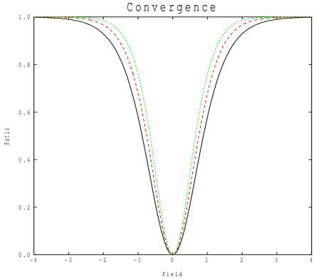
We perform a sequence of numerical calculations: For a chain of length we choose distinct values of and create distinct monodromy matrices. We then calculate our four quantities as a function of applied field for the set of all such conservation laws. Note that we choose to orthogonalise these conservation laws because of the additional stability this offers for the case when the conservation laws are over-complete. We then create new conservation laws by taking the distinct products of these monodromy matrices and include these in a larger calculation with both linear and quadratic combinations and calculate a second estimate to the Mazur inequality. We then calculate yet further conservation laws by taking the distinct triple products of these monodromy matrices and including them into a third Mazur estimate. We took this procedure to quartic order but proceeded no further. The results for a couple of representative cases, one metallic and one insulating, are provided in figure 1.
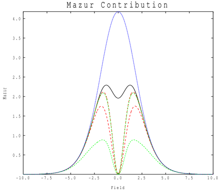
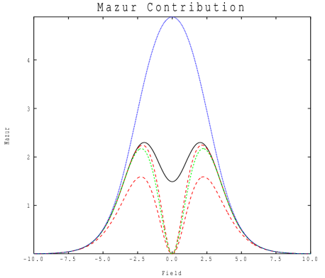
The conundrum is clearly observable: The contribution to the Mazur inequality from the conservation laws smoothly vanishes at zero field and some of the long-time residual is lost. For a finite system we can exhaust the attainable conservation laws and this observed loss is genuine! Fortunately, the resolution of this issue is straightforward: One important conservation law was missing from our analysis, , the -component of total-spin. The monodromy matrix is only non-degenerate when we additionally respect this symmetry too. Including this conservation law into our previous calculations, by including times the previous conservation laws as ‘independent’ laws, provides figure 2.
The problem at ‘half-filling’ has been alleviated and for small systems all the conservation laws can be exhausted and we can achieve the full long-time residual.
For the particular case of the XXZ model and the standard spin current, we now have an answer to our initial question: an initial current does decay as a function of time, except at =0 or , and the long-time residual is exhausted by the known conservation laws. In order to exhaust this residual one must include into the list of conservation laws, because without this law the residual is not exhausted and indeed at half-filling the local conservation laws offer nothing. Our results are for finite systems and there are definite problems in the thermodynamic limit. It is ‘known’z ; kluemper , from the Bethe Ansatz, that at half-filling the long-time residual shows interesting behaviour: For 1 we have a finite residual that smoothly vanishes as 1 and vanishes for 1. A single local conservation law must find difficulty in providing this behaviour and it is our need for the combination of with the local conservation laws which overcomes this difficulty.
Since any particular value of generically provides a non-degenerate monodromy matrix, we could have used a single such conservation law to exhaust the conserved current. We have demonstrated that this is so on very small systems, but the similarity of the laws provided by powers of this one law lead to unpleasant instability issues numerically, which, together with the added control of completeness issues, made our chosen procedure more effective.
Since we are dealing with the physical current in the system, but the fundamental theory should be applicable to an arbitrary operator, one can ask if the results are in any way special for the physical current. We repeated our calculations for the longer-range ‘currents’
| (62) |
where is the physical current and and are accessible to our available system sizes and they exhibit essentially no new physics at all: The operator is still available to show that the local conservation laws offer nothing in the absence of a field and the analogue plots to figure 2 are equivalent in all respects.
What can we say in general? At the formal level our results are clear: We see four natural quantities, , and in principle they are all distinct. The initial current, controlled by , only remains undiminished if the current operator is a conservation law itself, as happens for the case =0. The long-time residual, controlled by , may be considered to come from conservation laws, but only if we allow the inclusion of non-Abelian laws. If we have a set of mutually commuting conservation laws, then we only exhaust the long-time residual when the previously considered conserved current is the identity in the basis which diagonalises the conservation laws and also conserves any residual degeneracy.
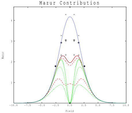
We have shown that the symmetry at zero field causes the local conservation laws to become independent from the conserved current and we have resolved this by including the -component of total-spin to successfully represent the entire conserved current, but all this was for finite systems: What happens in the thermodynamic limit? To exhaust the current conservation law we need to generate the long-time residual to machine accuracy from a Mazur calculation and this we can achieve with all accessible systems which do not have to be large to be convincing. To analyse the thermodynamic limit we need to finite-size scale and our relatively small systems are only indicative and not at all convincing. Nevertheless, we believe that in the thermodynamic limit the point at zero field becomes singular and that at all other fields the local conservation laws exhaust the conserved current. One analytical consideration is that in the thermodynamic limit we should get the same answer if we canonically fix the magnetisation or grand-canonically fix the field: Since when the magnetisation is fixed there is no difference between the conservation laws with and without magnetisation (except perhaps when the magnetisation vanishes), then there can only be one quantity generated by these laws, the full conserved current. We have incorporated the canonical calculations into figure 2 and it is plausible that they converge to the long-time residual. We have also finite-size scaled the fraction of the long-time residual provided by the conservation laws in figure 3
and it is easiest to believe that in the thermodynamic limit the point at zero magnetisation is an isolated puncture.
Although we appear to have a large number of degrees of freedom in our calculations (4096 for =12 for example) a brief analysis of the available degeneracy might suggest that our systems are too small to be relevant: Once we have extracted the degeneracy employing a field, although at first sight there appears to be a huge residual degeneracy, in fact this degeneracy is almost all lifted by inversion symmetry and the further residual degeneracy is woefully small! Indeed, we may employ the first non-trivial local conservation law, the energy currentznp , to lift the inversion symmetry and up to =11 this fully diagonalises the system. Additional degeneracy emerges for =12, but this is much less than is naively expected: We might expect that at order the distinct conservation laws were functionally independent, but for systems up to =11 all laws are describable as functions of the Hamiltonian, the energy current and the -component of total-spin! The role of degeneracy in the thermodynamic limit is currently not accessible to computers, even at the level of a hint!
For the Heisenberg model, we have established that for a finite system we can expect that
| (63) |
with
| (64) |
for some function of the relevant conserved quantities. The final issue is whether we can use this knowledge to prove the existence of a non-trivial long-time residual in the thermodynamic limit. Employing the first non-trivial conservation law, the heat current, it was shown that there is a non-vanishing residual at finite temperature for all fillings except half-fillingznp . As we have seen, at half-filling we also require to use the conservation law , so it seems plausible that we might be able to use a combination of both the heat current and the total spin to find the residual at half-filling. Unfortunately, this does not appear to be true and a verification of the long-time residual at half-filling using the Mazur inequality must await further investigation!
A natural technique is to Taylor expand the general conservation law and create a trivial conservation law from which the long-time residual can be deduced from the Mazur inequality
| (65) |
Clearly all the have the wrong symmetry and itself also has the wrong symmetry and so we might like to start from the law
| (66) |
for example. We can analyse this proposal in detail for the limit =0 where the Jordan-Wigner transformation reveals the solution as a non-interacting free-electron gas. Employing
| (67) | |||
we can verify that
| (68) |
with
| (69) |
at half-filling and does not vanish, as expected. Unfortunately, in the thermodynamic limit this conservation law offers nothing because it scales with the length of the chain but
| (70) |
scales with the square of the chain length rendering the contribution negligible! Note that the case =0 is special: There is a second ladder of conservation lawsgm which includes the current operator itself. When 0 the conservation laws
| (71) |
smoothly connect to the local conservation laws whilst the laws
| (72) |
are broken (except which is not part of the ladder). Noting the symmetries of these classes, the law
| (73) |
contributes from the appropriate sector and yields a finite Mazur contribution. This law arises from a linear superposition of the local conservation laws but it itself is clearly long-range.
One of the central current issues is that of finding a conservation law for which a single application of the Mazur inequality would provide incontrovertible proof of the existence of a long-time residual. We already know that this must be non-trivial for the current model, since the long-time residual is known to vanish for 1 and hence any prospective conservation law must respect this fact, a very non-analytic prospect. If we consider the generation of part of the long-time residual using a single conservation law, then we encounter an immediate problem if we attempt to employ local laws. If we consider the conservation law
| (74) |
where we require to use a local conservation law and the -component of total-spin, then we may replace this with
| (75) |
since neither operator has an overlap with the current on its own. Now the Mazur inequality tells us that
| (76) |
and note that, employing notation
| (77) |
we have
| (78) |
where the first term is likely to dominate. These ideas are essentially true whatever the operator , but if is local and the correlations in the system are short-range then we can deduce something from this: If we have that
| (79) |
for all such local operators then
| (80) |
and if and become far apart we might expect the correlations to become irrelevant. This correlation function might then be expected to scale linearly with system size. Similarly, including a then
| (81) |
also might be expected to scale linearly with system size. The consequence of this is that any local contribution to the Mazur inequality would be expected to vanish in the thermodynamic limit. In practice, the correlations are likely to be power-law in nature, but the physical idea behind the failure remains.
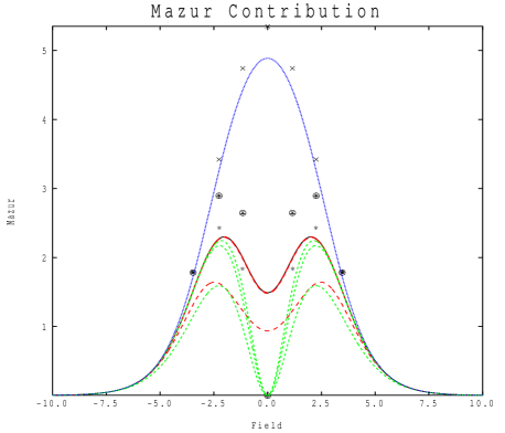
The hunt for an elementary conservation law that will provide a non-vanishing Mazur contribution at zero field probably necessitates non-local conservation laws, but we should remember that the monodromy matrix expanded in the manner that we employ does yield non-local lawsnonlocal and further we are complete for our finite systems so we employ an arbitrary linear superposition. Based on the previous limit of 0 we might suspect that it is only an arbitrary superposition over all lengths that is crucial and not the non-linear combinations of laws. Our final calculation offers a test of this idea through a finite-size scaling calculation of the fraction of the long-time residual provided by the linear conservation laws, the quadratic conservation laws and so on, order by order, in figure 4,

and unfortunately the contribution scales away, reinforcing the fear that a truly non-analytic function of the conservation laws is required.
IV Conclusions
Integrable systems can have anomalous conductivity, with currents flowing indefinitely once started. As suggested by Suzukisuzuki , this long-time residual can be thought of as some part of the current operator actually being one of the conservation laws of the system. We agree with this statement but refine one of the issues arising: Given a set of conservation laws, when is the conserved current either partially or wholly described by them. One might anticipate that a ‘complete set of mutually commuting’ conservation laws would generate all possible conservation laws, but this is incorrect: In general, additional independent conservation laws can exist with non-trivial commutation with the complete set. This is not just a formal issue, as can be seen by example: The isotropic Heisenberg model with the standard spin current. The local conservation laws do not completely diagonalise the system and there are a variety of ways of completing the conservation laws. We can simply diagonalise one of the components of total-spin as well, for example. If we choose to use the -component of total-spin then we can generate the full conserved current but if we choose either the - or -component of total spin then we can generate no long-time residual whatsoever! The current must be compatible with the complete set of mutually commuting conservation laws.
Using numerics on finite systems, we show how to generate the current conservation law for the XXZ model: If we combine the local conservation lawsgm with the -component of total spin then we can exhaust the long-time residual and consequently form the complete conserved current. Since the local conservation laws yield no long-time residual at all, in the absence of a field, any conservation law which has an overlap with the current must involve both the local conservation laws and the -component of total-spin.
The final issue addressed is as to the reason for the failure of any elementary conservation laws to provide even part of the conserved current for the case with no field. We observe that since we require to employ both a local conservation law and the -component of total-spin then for short-range interactions we need a coincidence of three local operators to yield a contribution and a consequent loss of this contribution in the thermodynamic limit. It is not easy to use the conservation laws to demonstrate a long-time residual in practice!
Acknowledgements.
We wish to acknowledge useful discussions with J.M.F. Gunn and C.A. Hooley. X.Z would like to acknowledge financial support by the E.U. grant MIRG-CT-2004-510543.References
- (1) R. S. MacKay, J. D. Meiss and I. C. Percival, Phys. Rev. Lett. 9, 697 (1984).
- (2) “Quantum Inverse Scattering Method and Correlation Functions”, V.E. Korepin, N.M. Bogoliubov and A.G. Izergin, Cambridge Univ. Press (1993).
- (3) M. P. Grabowski and P. Mathieu, Ann. Phys. 243, 299 (1996).
- (4) M.L.Mehta “Random matrices”, Academic Press, N.Y. (1967).
- (5) D.Poilblanc, T.Ziman, J.Bellisard, F.Mila, G.Montambaux, Europhys.Lett. 22,537 (1993).
- (6) X. Zotos and P. Prelovšek, in Interacting Electrons in Low Dimensions, Kluwer Academic Publishers (2003); arXiv:cond-mat/0304630.
- (7) A. V. Sologubenko et al., Phys. Rev. B 64, 054412 (2001).
- (8) D. Bernard, Int. J. Mod. Phys. BB7 3517 (1993).
- (9) M. Suzuki, Physica 51, 277 (1971).
- (10) X. Zotos, Phys. Rev. Lett. 82, 1764 (1999).
- (11) J. Benz, T. Fukui, A. Klümper, C. Scheeren, to be published in J. Phys. Soc. Jpn.
- (12) X. Zotos, F. Naef and P. Prelovšek, Phys. Rev. B55 11029 (1997).
- (13) P. Mazur, Physica 43, 533 (1969).
- (14) H. Bethe: Zeit. Phys. 71 (1931) 205.