Anomalous Hall effect in granular ferromagnetic metals
and effects of weak localization

Abstract

We theoretically investigate the anomalous Hall effect in a system of dense-packed ferromagnetic grains in the metallic regime. Using the formalism recently developed for the conventional Hall effect in granular metals, we calculate the residual anomalous Hall conductivity $\sigma_{xy}$ and resistivity $\rho_{xy}$ and weak localization corrections to them for both skew-scattering and side-jump mechanisms. We find that the scaling relation between $\rho_{xy}$ and the longitudinal resistivity $\rho_{xx}$ of the array does not hold, regardless of whether it is satisfied for the specific resistivities of the grain material or not. The weak localization corrections, however, are found to be in agreement with those for homogeneous metals. We discuss recent experimental data on the anomalous Hall effect in polycrystalline iron films in view of the obtained results.

I Introduction

The anomalous Hall effect (AHE) in ferromagnetic materials has been attracting the interest of researchers for decades. The first theoretical explanation Karplus and Luttinger (1954) of AHE was given by Karplus and Luttinger in 1954. They have shown that, in essence, the anomalous Hall current arises from the population imbalance of the electron spin states that is transferred into the asymmetry in electron motion via spin-orbit coupling. Since then, the theory of AHE has undergone further significant developments (see, e.g., recent reviews Wölfle and Muttalib, 2006 and Sinitsyn, 2008 and references therein). The interpretation Sundaram and Niu (1999) of AHE in terms of the Berry phase concept has fueled additional interestTaguchi et al. (2001); Jungwirth et al. (2002); Fang et al. (2003) to the problem.

One distinguishes between the intrinsic and extrinsic AHE. The intrinsic AHE arises in a perfect periodic lattice subject to spin-orbit coupling. It is due to the topological properties of the Bloch states and does not require any disorder. On the contrary, the extrinsic AHE is due to the asymmetric spin-orbit scattering of spin-polarized electrons on the impurities of the sample. Two mechanisms termed skew-scattering Smit (1958) and side-jump Berger (1970) are responsible for the extrinsic AHE. They depend differently on the amount of disorder in the sample and, as a result, for certain type of disorder the anomalous Hall (AH) resistivity scales linearly ($\rho_{xy}\propto\rho_{xx}$) with the longitudinal resistivity for the skew-scattering, and quadratically ($\rho_{xy}\propto\rho_{xx}^{2}$) for the side-jump mechanism. These scaling relations were observed experimentally Chien and Westgate (1980) in homogeneous systems. At the same time, for some heterostructure systems Xiong et al. (1992); Xu et al. (2008) considerable deviations from this scaling law were reported.

At sufficiently low temperatures, the physics of AHE is enriched by the quantum effects of Coulomb interactions and weak localization. The Coulomb interaction correction to the AH conductivity has been shown to vanish for both skew-scattering and side-jump mechanisms Langenfeld and Wölfle (1991); Muttalib and Wölfle (2007). Weak localization (WL) effects were studied in Refs. Langenfeld and Wölfle, 1991; Dugaev et al., 2001; Muttalib and Wölfle, 2007 and it was demonstrated that WL correction to AH conductivity is nonzeroLangenfeld and Wölfle (1991); Dugaev et al. (2001); Muttalib and Wölfle (2007) for skew-scattering and vanishes Dugaev et al. (2001); Muttalib and Wölfle (2007) for side-jump mechanism. The logarithmic temperature dependence of the AH resistivity and the absence of such for the AH conductivity observed in amorphous iron films Bergmann and Ye (1991) were initially attributed to the Coulomb interactions Langenfeld and Wölfle (1991) and later interpreted Dugaev et al. (2001) in terms of the WL corrections for the side-jump mechanism.

In a recent paper Mitra et al. (2007), the logarithmic temperature dependence of the longitudinal and AH resistivities of the polycrystalline iron films at sufficiently low temperatures was reported. For well-conducting samples, the behavior could be well explained by the WL theory Langenfeld and Wölfle (1991); Dugaev et al. (2001) of the AHE in two-dimensional homogeneously disordered samples. For more resistive samples, however, noticeable deviations from the theoretical predictions were observed. The authors suggested that these deviations could be attributed to the granular structure of the samples.

Motivated by the experimental data of Ref. Mitra et al., 2007, in the present paper we investigate AHE in a granular system of ferromagnetic metallic nanoparticles within a microscopic theory. For that purpose, we extended the recently developed theory Kharitonov and Efetov (2007, 2008) of the conventional Hall effect in granular metals to describe AHE.

The paper is organized as follows. In Sec. II, we formulate the model for a granular system. In Sec. III, the residual AH resistivity is calculated, first using the classical approach, and then this result is recovered from the diagrammatic approach. The breakdown of the scaling relation between the AH and longitudinal resistivities is discussed. In Sec. IV, we calculate the WL corrections to the AH resistivity and discuss the experiment of Ref. Mitra et al., 2007. Concluding remarks are presented in Sec. V.

II Model

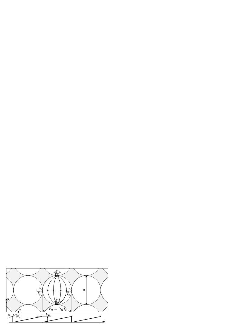
Figure 1: Granular system and the classical picture of the Hall conductivity. The external Ohmic voltage $V_{y}$ is applied to the contacts in the $y$ direction. The resulting Ohmic current $I_{y}=G_{T}V_{y}$ running through the grain in the $y$ direction causes the Hall voltage drop $V_{H}=R_{H}I_{y}$ between its opposite banks in the $x$ direction. Since when calculating the Hall conductivity $\sigma_{xy}$ the total voltage drop per lattice period in the $x$ direction is assumed 0, the Hall voltage $V_{H}$ is applied with an opposite sign to the contacts in the $x$ direction (see bottom), causing the Hall current $I_{x}=G_{T}V_{H}=G_{T}^{2}R_{H}V_{y}$ [see Eq. (8)].

We consider a regular quadratic ($d=2$, single granular monolayer) or cubic ($d=3$, many monolayers) lattice of identical in form and size three-dimensional metallic grains coupled to each other by tunnel contacts with identical conductances $G_{T}$. At the same time, we assume that the grains are disordered either due to impurities in the bulk of the grains or due to an atomically irregular shape. The assumptions of the regularity of the system simplify the analysis significantly, but are not crucial. The results we obtain are expected to apply to structurally disordered granular arrays as well. We consider the metallic regime in this paper, when the tunnel conductance $G_{T}=(2e^{2}/\hbar)g_{T}$ is much larger than the quantum conductance,

$$g_{T}\gg 1.$$ (1)

In this limit, the whole granular system is a good conductor and the quantum effects of weak localization and Coulomb interactions can be studied Beloborodov et al. (2007) perturbatively in $1/g_{T}\ll 1$. As usual, it is assumed that the granularity is well-pronounced Beloborodov et al. (2007), i.e., the dimensionless grain conductance $g_{0}$ exceeds the tunnel conductance $g_{T}$,

$$g_{0}\gg g_{T}.$$ (2)

The key ingredients of AHE that give rise to a finite transversal conductivity $\sigma_{xy}$ are (i) the spin magnetization of conduction electrons and (ii) considerable spin-orbit interaction. Analogously to homogenously disordered metals, the simplest Hamiltonian containing these two ingredients and thus describing AHE in a granular system can be written as

$$\hat{H}=\hat{H}_{0}+\hat{H}_{U}+\hat{H}_{T}.$$ (3)

The first two terms in Eq. (3) describe isolated grains, where

$$\hat{H}_{0}=\sum\limits_{\mathbf{i}}\int\mathrm{d}\mathbf{r}_{\mathbf{i}}\,\Psi^{\dagger}(\mathbf{r}_{\mathbf{i}})\left[-\frac{\nabla_{\mathbf{r}_{\mathbf{i}}}^{2}}{2m}-\epsilon_{F}-\left(\mathbf{h}\cdot\bm{\sigma}\right)\right]\Psi(\mathbf{r}_{\mathbf{i}})$$ (4a)

contains the kinetic energy and the exchange field $${\bf h}=h{\bf e}_{z} z \hbar=1$$ directed along the axis in all the grains (we put ). The exchange field causes a finite spin magnetization of the electrons. The intragrain disorder is described by

$$\hat{H}_{U} = \sum\limits_{\mathbf{i}}\int\mathrm{d}\mathbf{r}_{\mathbf{i}}\Psi^{\dagger}(\mathbf{r}_{\mathbf{i}})\left\{U(\mathbf{r}_{\mathbf{i}})\right.$$ (4b)

$$\left.-\mathrm{i}\lambda^{2}\left(\bm{\sigma}\cdot\left[\nabla U(\mathbf{r}_{\mathbf{i}})\times\nabla_{\mathbf{r}_{\mathbf{i}}}\right]\right)\right\}\Psi(\mathbf{r}_{\mathbf{i}}),$$

where the first term corresponds to the conventional scattering on the disorder potential $$U({\bf r}_{\bf i}) \Psi=\left(\psi_{\uparrow},\psi_{\downarrow}\right)^{\textsf{T}} \bm{\sigma}=(\sigma_{x},\sigma_{y},\sigma_{z}) \sigma_{\alpha} \alpha=x,y,z \mathbf{i}=(i_{1},\ldots,i_{d}) {\bf r}_{\bf i} \mathbf{i}$$ and the second one to the spin-orbit scattering. In Eqs. (4a) and (4b), is the two-component spinor field operator of the electrons, denotes the vector consisting of the Pauli matrices , , and is an integer tuple numerating the grains on the lattice. The integration with respect to is performed over volume of the grain .

We consider the simplest model of disorder

$$U({\bf r})=\sum_{a}u\delta({\bf r}-{\bf r}_{a}),$$ (4c)

in which the point impurities are located at random positions ${\bf r}_{a}$ within the grains and are uniformly distributed with the concentration $n_{\text{i}}$ over the volume of the grains. We assume that spin-orbit coupling is weak in the sense $\lambda p_{\mathrm{F}}\ll 1$, where $p_{F}$ is the Fermi momentum, and that the exchange field $h\ll\epsilon_{F}$ is smaller than the Fermi energy $\epsilon_{F}$ of electrons in the grains. The latter two assumptions allow one to study AHE perturbatively in $h$ and spin-orbit coupling.

The last term in the Hamiltonian (3) describes tunneling between the grains,

$$\hat{H}_{T} = \sum\limits_{\left\langle{\bf i},{\bf j}\right\rangle}(X_{{\bf i},{\bf j}}+X_{{\bf j},{\bf i}}),$$

$$X_{{\bf i},{\bf j}} = \int\mathrm{d}{\bf s}_{\bf i}\mathrm{d}{\bf s}_{\bf j}\,t(\mathbf{s}_{\mathbf{i}},\mathbf{s}_{\bf j})\Psi^{\dagger}(\mathbf{s}_{\mathbf{i}})\Psi(\mathbf{s}_{\mathbf{j}}).$$ (4d)

The summation in Eq. (4d) is done over the neighboring grains ${\bf i}$ and ${\bf j}$, so that each tunnel contact is counted only once, and the integration with respect to ${\bf s}_{\bf i}$ and ${\bf s}_{\bf j}$ is performed over two surfaces of the contact between the grains ${\bf i}$ and ${\bf j}$, one belonging to grain $\mathbf{i}$ and the other to grain $\mathbf{j}$. It is both physically reasonable and convenient for calculations Kharitonov and Efetov (2008) to treat the tunneling amplitudes $t(\mathbf{s}_{\mathbf{i}},\mathbf{s}_{\mathbf{j}})$ as Gaussian random variables with the variance $\langle t(\mathbf{s}_{\mathbf{i}},\mathbf{s}_{\mathbf{j}})t(\mathbf{s}_{\mathbf{j}},\mathbf{s}_{\mathbf{i}})\rangle_{t}=t_{0}^{2}\,\delta(\mathbf{s}_{\mathbf{i}}-\mathbf{s}_{\mathbf{j}})$.

The anomalous Hall conductivity of the array is calculated using the Kubo formula for granular systems in the Matsubara representation,

$$\sigma_{{\bf a}{\bf b}}(\omega)=a^{2-d}\frac{1}{\omega}\left[\Pi_{{\bf a}{\bf b}}(\omega)-\Pi_{{\bf a}{\bf b}}(0)\right],$$ (5)

where

$$\Pi_{{\bf a}{\bf b}}(\omega)=-\sum_{\bf j}\int_{0}^{1/T}\mathrm{d}\tau\,\mathrm{e}^{\mathrm{i}\omega\tau}\langle\mathrm{T}_{\tau}[I_{{\bf i},{\bf a}}(\tau)I_{{\bf j},{\bf b}}(0)]\rangle$$ (6)

is the correlation function of the tunnel currents

$$I_{{\bf i},{\bf a}}=-\mathrm{i}e(X_{{\bf i}+{\bf a},{\bf i}}-X_{{\bf i},{\bf i}+{\bf a}}).$$ (7)

Here, $\omega$ is a bosonic Matsubara frequency (we assume $\omega>0$ throughout the paper), the lattice unit vectors ${\bf a}$ and ${\bf b}$ denote the directions of the current and external electric field, respectively. The approach to calculating the AH conductivity is analogous to that developed for the ordinary Hall effect in Ref. Kharitonov and Efetov, 2008. It is based on the diagrammatic perturbation theory in the tunnel Hamiltonian (4d) with the ratio $g_{T}/g_{0}$ [Eq. (2)] of the tunnel and grain conductances as an expansion parameter. We refer the reader to Ref. Kharitonov and Efetov, 2008 for the details of the approach.

In our model (3)-(4d), the source of spin-orbit scattering are the impurities in the bulk of the grains [second term in Eq. (4b)]. The anomalous Hall current, therefore, arises from the bulk of the grains. To perform explicit calculations, we will assume the intragrain dynamics is diffusive, i.e., the mean free path $l\ll a$ is much smaller than the grain size $a$. In the opposite case of clean grains, surface scattering is dominant and spin-orbit scattering off the grain boundary could be the major source of AHE. If the boundary roughness can effectively be modeled by scattering on impurities in the bulk of the grains, our results may also be applicable to the arrays of ballistic grains with chaotic intragrain dynamics.

III Residual anomalous Hall resistivity

III.1 Classical approach

We start by calculating the residual anomalous Hall conductivity $\sigma_{xy}$ and resistivity $\rho_{xy}$ of a granular array, neglecting quantum effects of weak localization and Coulomb interactions. Actually, as we show in this subsection, as long as quantum effects are neglected the AH conductivity can be obtained by means of the classical electrodynamics without using the Kubo formula. The diagrammatic approach that will further allow us to include quantum effects is presented in Sec. III.3.

Within the classical approach, the granular array can be considered as a resistor network with the tunnel contacts viewed as surface resistors with conductance $G_{T}$. The AHE occurs inside the grains and is fully characterized by the AH resistance $R_{H}$ of the each grain. Given $R_{H}$, in the leading order in $g_{T}/g_{0}\ll 1$, one can easily arrive (Fig. 1) at the expression

$$\sigma_{xy}=a^{2-d}G_{T}^{2}R_{H}$$ (8)

for the residual AH conductivity of the granular array. Since the longitudinal conductivity equals

$$\sigma_{xx}=a^{2-d}G_{T},$$ (9)

for the AH resistivity of the granular system we obtain

$$\rho_{xy}=\frac{\sigma_{xy}}{\sigma_{xx}^{2}}=a^{d-2}R_{H}.$$ (10)

The AH resistivity is, therefore, expressed solely through the Hall resistance $R_{H}$ of a single grain and is independent of the tunnel conductance $G_{T}$, which determines the longitudinal resistivity [Eq. (9)].

To get a further insight into the problem, one should specify $R_{H}$ more explicitly. The electron transport in the diffusive grains can fully be described by the specific longitudinal $\sigma_{xx}^{\text{gr}}$ and AH $\sigma_{xy}^{\text{gr}}$ conductivities of the grain material. The AH conductivity

$$\sigma_{xy}^{\text{gr}}=\sigma_{xy}^{\text{gr,ss}}+\sigma_{xy}^{\text{gr,sj}}$$ (11)

is a sum of two contributions due to skew-scattering (ss) and side-jump (sj) mechanisms. Given $\sigma_{xx}^{\text{gr}}$ and $\sigma_{xy}^{\text{gr}}$, one can find the anomalous Hall resistance $R_{H}$ of the grain by solving the electrodynamics problem for the distribution of the electric potential in the grain Kharitonov and Efetov (2008). Analyzing this problem, one obtains that $R_{H}$ is expressed through the specific AH resistivity of the grain material $\rho_{xy}^{\text{gr}}=\sigma_{xy}^{\text{gr}}/(\sigma_{xx}^{\text{gr}})^{2}$ in the following way

$$R_{H}=A_{H}\rho_{xy}^{\text{gr}}/a,$$ (12)

where the numerical factor $A_{H}\leq 1$ is determined by the shape of the grain only. For simple grain geometries $A_{H}$ can be found explicitly, e.g., $A_{H}=1$ for cubic and $A_{H}=\pi/4$ for spherical grains.

As follows from Eqs. (10) and (12), the AH resistivity of a three-dimensional granular array ($d=3$, many grain monolayers)

$$\rho_{xy}=A_{H}\rho_{xy}^{\text{gr}}$$ (13)

is determined by the AH resistivity of the grain material, up to a geometrical numerical factor determined by the shape of the grain. The AH resistivity of a granular film ($d=2$, one to several monolayers)

$$\rho_{xy}=A_{H}\rho_{xy}^{\text{gr}}/d_{z}$$ (14)

is obtained by dividing the 3D result (13) by the thickness $d_{z}$ of the film.

The results (8)-(14) are actually analogous to those obtained in Refs. Kharitonov and Efetov, 2007 and Kharitonov and Efetov, 2008 for the conventional Hall effect in granular metals, with the AH resistivity of the grain material $\rho_{xy}^{\text{gr}}$ entering the equations instead of the conventional Hall resistivity. Specifics of AHE is reflected in, e.g., the breakdown of the scaling relation between the AH and longitudinal resistivities, as discussed in the next subsection.

III.2 Breakdown of the scaling relation

In homogeneously disordered systems, for certain types of disorder the AH and longitudinal resistivities obey the scaling relation

$$\rho_{xy}\propto\rho_{xx}^{\gamma}$$ (15)

with the exponent $\gamma=1$ for skew-scattering and $\gamma=2$ for side-jump mechanisms. This scaling originates from the fact that spin-orbit scattering, which results in the transversal current, is caused by the same impurity potential $U({\bf r})$ [Eq. (4b)], scattering off which is responsible for the finite longitudinal resistivity.

The scaling relation (15) holds for the model of identical randomly placed short-range impurities, described by Eqs. (4b) and (4c). Within this model, the longitudinal and AH conductivities of the grain material equal

$$\sigma_{xx}^{\text{gr}}=\frac{e^{2}v_{F}^{2}}{3\pi n_{\text{i}}u^{2}},$$ (16)

$$\sigma_{xy}^{\text{gr,ss}}=-\frac{5\pi}{3}\nu u(\lambda p_{F})^{2}\frac{h}{\epsilon_{F}}\sigma_{xx}^{\text{gr}},$$ (17)

$$\sigma_{xy}^{\text{gr,sj}}=-3\pi(\nu u)^{2}\frac{n_{\text{i}}}{\nu\epsilon_{F}}(\lambda p_{F})^{2}\frac{h}{\epsilon_{F}}\sigma_{xx}^{\text{gr}}.$$ (18)

Here, $\nu$ is the density of states at the Fermi level for $h=0$. As seen from Eqs. (16)-(18), as the impurity concentration $n_{\text{i}}$ is varied, the resistivities $\rho_{xx}^{\text{gr}}=1/\sigma_{xx}^{\text{gr}}$ and $\rho_{xy}^{\text{gr}}$ indeed change according to Eq. (15) [it is implied in Eq. (15) that the variation of $\rho_{xy}^{\text{gr}}$ and $\rho_{xx}^{\text{gr}}$ is caused by the change of $n_{\text{i}}$, i.e., the amount of disorder, whereas the strength $u$ of the scattering potential of single impurities is fixed]. The scaling relation (15) thus holds for the specific resistivities of the grain material. Although Eqs. (16)-(18) are obtained for weak impurity scattering (Born approximation), it can be shown Muttalib and Wölfle (2007) that the scaling law (15) holds for strong scattering as well, since the dependence on the impurity concentration remains the same. However, for more complicated type of disorder with stronger finite-range correlations of the disorder potential the scaling relation may be violated.

Comparing Eqs. (9) and (10), we see that no scaling relation similar to (15) between the AH $\rho_{xy}$ and longitudinal

$$\rho_{xx}=a^{d-2}/G_{T}$$ (19)

resistivities of the whole granular array holds. This result is actually not surprising, since the longitudinal and AH transport in granular systems are governed by different mechanisms: the former is due to tunneling through the potential barriers between the grains, whereas the latter is caused by spin-orbit scattering inside the grains. According to Eqs. (9) and (10), if the granularity is indeed pronounced [Eq. (2)], the AH resistivity should not vary much for samples with noticeably different longitudinal resistivities. One could say that for granular systems, the scaling relation (15) with the exponent $\gamma=0$ holds, independent of the dominant mechanism of AHE. In this context, we note that considerable deviations from the scaling law (15) have previously been observed experimentally in several types of heterostructure systems Xiong et al. (1992); Xu et al. (2008), in which the longitudinal resistivity was also governed by the structural disorder (such as transparency of the interfaces) rather than by the intrinsic disorder of the ferromagnetic material.

III.3 Residual anomalous Hall resistivity via diagrammatic approach

The classical approach allows one to easily obtain Eq. (8) for the residual AH conductivity and make some interesting conclusions about AH transport in granular metals at high enough temperatures. However, it has nothing to say about quantum effects of weak localization and Coulomb interactions, which set in at sufficiently low temperatures. To study these effects on the AH transport, a more sophisticated diagrammatic approach based on the Kubo formula (5) is needed. Before we proceed with the quantum effects in Sec. IV, we first demonstrate here how the classical result (8) is reproduced within the diagrammatic approach.

As demonstrated in Ref. Kharitonov and Efetov, 2008, the key object of the diagrammatic approach to the Hall effect in granular systems is the intragrain diffuson, i.e., the two-particle electron propagator of an isolated grain. It contains all the information about the specific mechanism of the Hall effect. As usual, the diffuson is formally defined as the disorder-averaged product of two Greens’s functions. In the presence of the exchange field and spin-orbit scattering the electron Green’s functions are matrices in the spin space and the intragrain diffuson is defined as their direct product,

$$\hat{D}_{\omega}({\bf r},{\bf r}^{\prime})=\frac{1}{2\pi\nu}\langle\hat{\mathcal{G}}_{\varepsilon+\omega}({\bf r},{\bf r}^{\prime})\otimes\hat{\mathcal{G}}_{\varepsilon}({\bf r}^{\prime},{\bf r})\rangle_{U},\mbox{ }(\varepsilon+\omega)\varepsilon<0$$ (20)

Here, $\hat{\mathcal{G}}$’s are the exact Green’s functions of the intragrain Hamiltonian $\hat{H}_{0}+\hat{H}_{U}$ in the Matsubara technique for a given realization of the disorder potential $U({\bf r})$ and the angle brackets $\langle\ldots\rangle_{U}$ denote disorder-averaging.

According to the Kubo formula (5), the conductivity is in the leading order expressed through the spin-singlet diffuson component, which is given by the trace $\text{Tr}_{\sigma}$ of the Green’s functions in the spin space

$$D_{\omega}(\mathbf{r},\mathbf{r}^{\prime})=\frac{1}{4\pi\nu}\langle\text{Tr}_{\sigma}[\hat{\mathcal{G}}_{\varepsilon+\omega}({\bf r},{\bf r}^{\prime})\hat{\mathcal{G}}_{\varepsilon}({\bf r}^{\prime},{\bf r})]\rangle_{U},\mbox{ }(\varepsilon+\omega)\varepsilon<0.$$ (21)

Below, we will need the spin-singlet diffuson (21) only.

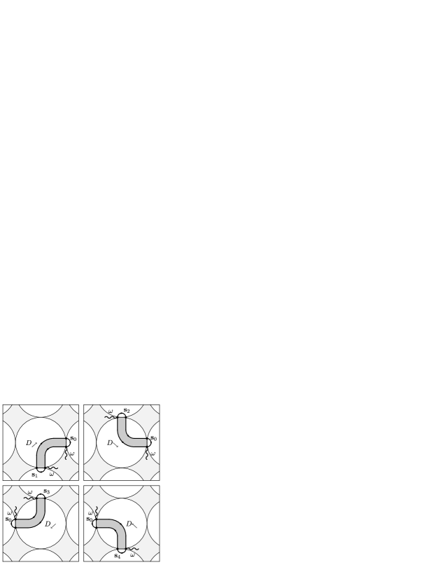
Figure 2: Diagrams for the residual anomalous Hall conductivity $\sigma_{xy}$ [Eqs. (8) and (22)], see Ref. Kharitonov and Efetov, 2008 for details.

Analogously to the conventional Hall effect Kharitonov and Efetov (2007, 2008), the residual AH conductivity $\sigma_{xy}$ is given by the diagrams in Fig. 2. Calculating these diagrams, one can relate the tunnel conductance in Eq. (8) for $\sigma_{xy}$ to the microscopic parameters of the model as $g_{T}=2\pi(\nu t_{0})^{2}S_{0}$ ($S_{0}$ is the area of the contact) and express the AH resistance of the grain through to the intragrain diffuson (21) as

$$R_{H}=\frac{1}{2e^{2}\nu}(D_{\nearrow}-D_{\searrow}+D_{\swarrow}-D_{\nwarrow}),$$ (22)

where

$$D_{\alpha}=\frac{1}{S_{0}^{2}}\int\mathrm{d}{\bf s}_{0}\mathrm{d}{\bf s}_{a}D_{\omega=0}({\bf s}_{0},{\bf s}_{a})$$ (23)

are the diffusons at zero frequency $\omega=0$ connecting different contacts as shown in Fig. 2, with $a=1,2,3,4$ for $\alpha=\nearrow,\searrow,\swarrow,\nwarrow$, respectively.

The problem of calculating $R_{H}$ is, therefore, reduced to finding the diffuson. Within the conventional disorder-averaging technique Abrikosov et al. (1965), the diffuson (21) can be shown to satisfy the diffusion equation

$$(\omega-D_{0}\nabla_{\mathbf{r}}^{2})D_{\omega}(\mathbf{r},\mathbf{r}^{\prime})=\delta(\mathbf{r}-\mathbf{r}^{\prime}),$$ (24)

in which $D_{0}=v_{F}^{2}\tau/3$ is the coefficient of the intragrain diffusion ($v_{F}$ is the Fermi velocity and $\tau$ is the scattering time, $1/\tau=2\pi\nu n_{\text{i}}u^{2}$). Equation (24) itself clearly does not contain any information about the Hall effect. This information is contained in the boundary condition for $D_{\omega}({\bf r},{\bf r}^{\prime})$, which Eq. (24) must be supplied with for a finite system. In Ref. Kharitonov and Efetov, 2008 a general method of deriving the boundary condition for the diffuson was developed and it was shown that the boundary condition may be written as

$$n_{\alpha}\langle j_{\alpha}r_{\beta}\rangle\nabla_{{\bf r}\beta}D_{\omega}({\bf r},{\bf r}^{\prime})|_{{\bf r}\in S}=0.$$ (25)

Here, $\alpha,\beta=x,y,z$, and $n_{\alpha}$ are the components of the unit vector $\mathbf{n}$ normal to the grain boundary $S$ at point ${\bf r}$ and pointing out of the grain. In Eq. (25),

$$\langle j_{\alpha}r_{\beta}\rangle=\frac{1}{2}\text{Tr}_{\sigma}\int\mathrm{d}{\bf r}^{\prime}\,\langle\hat{j}_{{\bf r}\alpha}[\mathcal{G}_{\varepsilon+\omega}({\bf r},{\bf r}^{\prime})\mathcal{G}_{\varepsilon}({\bf r}^{\prime},{\bf r})]({\bf r}^{\prime}-{\bf r})_{\beta}\rangle_{U}$$ (26)

is the current-coordinate correlation function. The nonrelativistic part of the current operator $\hat{{\bf j}}$ has the conventional form

$$\hat{{\bf j}}[\psi^{*}({\bf r}),\psi({\bf r})]=\frac{-\mathrm{i}}{2m}[\psi^{*}({\bf r})\nabla\psi({\bf r})-\psi({\bf r})\nabla\psi^{*}({\bf r})]$$ (27)

Explicit form of the boundary condition (25) is thus determined solely by $\langle j_{\alpha}r_{\beta}\rangle$. Analogously to the conductivity tensor, only the longitudinal $\langle j_{x}r_{x}\rangle=\langle j_{y}r_{y}\rangle=\langle j_{z}r_{z}\rangle$ and Hall $\langle j_{x}r_{y}\rangle=-\langle j_{y}r_{x}\rangle$ components are nonzero (we remind the reader that the exchange field is directed along the $z$ axis). This allows us to rewrite Eq. (25) in the form

$$\langle j_{x}r_{x}\rangle({\bf n}\cdot\nabla_{{\bf r}}D_{\omega}({\bf r},{\bf r}^{\prime}))|_{{\bf r}\in S}=\langle j_{x}r_{y}\rangle({\bf t}\cdot\nabla_{{\bf r}}D_{\omega}({\bf r},{\bf r}^{\prime}))|_{{\bf r}\in S},$$ (28)

where the vector ${\bf t}=[{\bf n}\times{\bf h}]/h$ is tangent the grain boundary at point ${\bf r}$.

Since the AHE is weak due to the smallness of the spin-orbit coupling constant $\lambda p_{F}\ll 1$ and the exchange field $h/\epsilon_{F}\ll 1$, the longitudinal component $\langle j_{x}r_{x}\rangle$ can be calculated neglecting the exchange field and spin-orbit scattering completely and the expression for it reads

$$\left\langle j_{x}r_{x}\right\rangle=-\frac{4\pi}{3}\nu l^{2}.$$ (29)

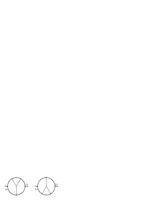
Figure 3: Diagrams for the Hall component $\langle j_{x}r_{y}\rangle^{\text{ss}}$ of the current-coordinate correlation function (26) due to the skew-scattering mechanism.

All specifics of the AHE is contained in the Hall component $\langle j_{x}r_{y}\rangle$. Analogously to the AH conductivity of a homogeneously disordered metal [see Eqs. (11), (17) and (18)], the total Hall correlation function

$$\langle j_{x}r_{y}\rangle=\langle j_{x}r_{y}\rangle^{\text{ss}}+\langle j_{x}r_{y}\rangle^{\text{sj}}$$ (30)

is the sum of two contributions due to skew-scattering (ss) and side-jump (sj) mechanisms.

The skew-scattering part $\left\langle j_{x}r_{y}\right\rangle^{\mathrm{ss}}$ is given by the diagrams in Fig. 3, which contain the impurity lines describing the third-order scattering processes on a single impurity, see, e.g., Ref. Wölfle and Muttalib, 2006. Calculating these diagrams, we obtain

$$\left\langle j_{x}r_{y}\right\rangle^{\mathrm{ss}}=-\frac{5\pi}{3}\nu u(\lambda p_{F})^{2}\frac{h}{\epsilon_{F}}\left\langle j_{x}r_{x}\right\rangle.$$ (31)

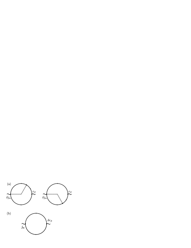
Figure 4: Diagrams for Hall component $\langle j_{x}r_{y}\rangle^{\text{sj}}$ of the current-coordinate correlation function (26) due to the side-jump mechanism. Diagrams (a) and (b) contain the relativistic corrections to the current [$\delta\hat{{\bf j}}$, Eq. (32)] and coordinate [$\delta\hat{{\bf r}}$, Eq. (33)] vertices, respectively.

The diagrams for the side-jump contribution $\left\langle j_{x}r_{y}\right\rangle^{\mathrm{sj}}$ are shown in Fig. 4. The diagram in Fig. 4 (a) contains the conventional for the side-jump mechanism relativistic correction

$$\delta\hat{{\bf j}}=\lambda^{2}\left[\bm{\sigma}\times\nabla U(\mathbf{r})\right],$$ (32)

to the current operator (27), see, e.g., Ref. Wölfle and Muttalib, 2006. Additionally, there exists an analogous relativistic correction to the coordinate vertex. This contribution can be obtained by repeating the derivation of the boundary condition (25) done in Ref. Kharitonov and Efetov, 2008, but taking into account the spin-orbit term of $\hat{H}_{U}$ [Eq. (4b)] in the diffuson ladder. This gives the diagram in Fig. 4 (b), in which

$$\delta\hat{{\bf r}}=\lambda^{2}[\bm{\sigma}\times\hat{{\bf p}}]$$ (33)

is the relativistic correction to the coordinate operator ($\hat{{\bf p}}=-\text{i}\nabla$). One can recognize that $\delta\hat{{\bf r}}$ is the operator of the lateral translation (“side-jump”), see, e.g. Ref. Crépieux and Bruno, 2001. Calculating the diagrams in Fig. 4, we obtain

$$\left\langle j_{x}r_{y}\right\rangle^{\mathrm{sj}}=-3\pi(\nu u)^{2}\frac{n_{\text{i}}}{\nu\epsilon_{F}}(\lambda p_{F})^{2}\frac{h}{\epsilon_{F}}\left\langle j_{x}r_{x}\right\rangle.$$ (34)

Comparing Eqs. (29), (31) and (34) with Eqs. (16), (17) and (18), we note that for both skew-scattering and side-jump contributions the relation

$$\frac{\left\langle j_{x}r_{y}\right\rangle^{\mathrm{ss/sj}}}{\left\langle j_{x}r_{x}\right\rangle}=\frac{\sigma^{\mathrm{gr},\mathrm{ss/sj}}_{xy}}{\sigma^{\mathrm{gr}}_{xx}}$$ (35)

holds. Therefore the boundary condition (25) may be rewritten as

$$\sigma_{xx}^{\text{gr}}({\bf n}\cdot\nabla_{{\bf r}}D_{\omega}({\bf r},{\bf r}^{\prime}))|_{{\bf r}\in S}=\sigma_{xy}^{\text{gr}}({\bf t}\cdot\nabla_{{\bf r}}D_{\omega}({\bf r},{\bf r}^{\prime}))|_{{\bf r}\in S}.$$ (36)

As shown in Ref. Kharitonov and Efetov, 2008, it is exactly this form of the boundary condition, which is necessary to reproduce the classical result (12) for the Hall resistance $R_{H}$ obtained by solving the electrodynamics problem.

Having established the correspondence between the classical and diagrammatic approaches, comparing Eqs. (22), (24), and (28) with Eq. (12) and using the Einstein relation $\sigma_{xx}^{\text{gr}}=2e^{2}\nu D_{0}$, we can express the Hall resistance of the grain as

$$R_{H}=A_{H}\frac{1}{2e^{2}\nu}\frac{\langle j_{x}r_{y}\rangle}{\langle j_{x}r_{x}\rangle}\frac{1}{D_{0}a}$$ (37)

This form will be used in the next section for calculating WL corrections.

IV Weak localization corrections

IV.1 Calculations

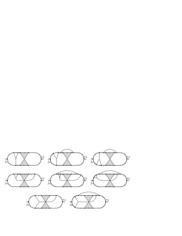
Figure 5: Diagrams for the weak localization correction $\delta\langle j_{x}r_{y}\rangle^{\text{ss}}$ to the skew-scattering Hall component $\langle j_{x}r_{y}\rangle^{\mathrm{ss}}$ [Eq. (31)] of the current-coordinate correlation function (26). The gray regions denote the Cooperons [Eq. (40)]. Each diagram depicted above stands for four diagrams: the ones not shown are obtained by reflecting the impurity lines through the diagram center and/or flipping the diagram upside-down.

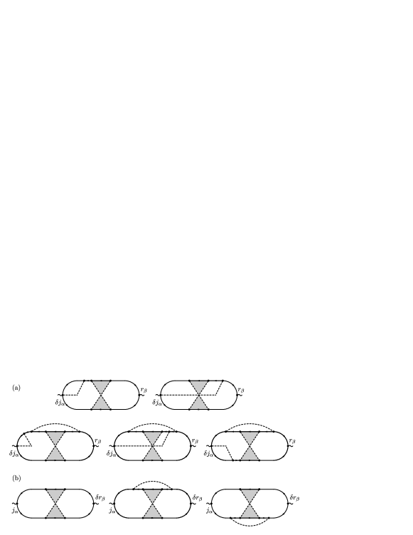
Figure 6: Diagrams for the weak localization correction $\delta\langle j_{x}r_{y}\rangle^{\text{ss}}$ to the side-jump Hall component $\langle j_{x}r_{y}\rangle^{\mathrm{sj}}$ [Eq. (34)] of the current-coordinate correlation function (26). Diagrams (a) and (b) contain the relativistic corrections to the current [$\delta\hat{{\bf j}}$, Eq. (32)] and coordinate [$\delta\hat{{\bf r}}$, Eq. (33)] vertices, respectively. Each diagram in panel (a) stands for two diagrams: the one not shown is obtained by flipping the diagram upside-down.

We now proceed with calculating the weak localization corrections to the obtained “classical” anomalous Hall conductivity (8) and resistivity (10) of the granular metal.

Technically, one has to consider WL corrections to the diagrams in Fig. 2 for the bare Hall conductivity (8) by inserting the Cooperon ladders into them in all possible ways. As shown in Ref. Kharitonov and Efetov, 2008, such WL corrections are factorized according to the form Eq. (8), i.e., there are diagrams describing the corrections to the tunnel conductance $G_{T}$ only and to the Hall resistance $R_{H}$ of the grain only. This allows one to write down the total weak localization correction $\delta\sigma_{xy}$ to AH conductivity $\sigma_{xy}$ in the form

$$\frac{\delta\sigma_{xy}}{\sigma_{xy}}=2\frac{\delta G_{T}}{G_{T}}+\frac{\delta R_{H}}{R_{H}}$$ (38)

Naturally, the WL correction $\delta G_{T}$ to the tunneling conductance has the same form as that to the longitudinal conductivity $\sigma_{xx}$ [Eq. (9)] Beloborodov et al. (2004); Biagini et al. (2005) and reads

$$\frac{\delta G_{T}}{G_{T}}=\frac{\delta\sigma_{xx}}{\sigma_{xx}}=\frac{\Delta}{2\pi}[C_{\omega=0}({\bf i}+{\bf a},{\bf i})+C_{\omega=0}({\bf i},{\bf i}+{\bf a})]$$ (39)

Here,

$$C_{\omega}({\bf i},{\bf j})=\int\frac{a^{d}\mathrm{d}^{d}\mathbf{q}}{(2\pi)^{d}}\frac{\mathrm{e}^{\mathrm{i}a({\bf q}\cdot({\bf i}-{\bf j}))}}{\omega+2\Gamma\sum_{\alpha}[1-\cos(q_{\alpha}a)]+1/\tau_{\varphi}}$$ (40)

is the Cooperon of the whole granular array calculated in the zero-mode approximation for the intragrain Cooperons Beloborodov et al. (2001, 2004); Biagini et al. (2005), $\Delta$ is the mean level spacing in the grain, and ${\bf a}={\bf e}_{x}$ or ${\bf a}={\bf e}_{y}$. In Eq. (40), $\Gamma=g_{T}\Delta$ is the tunneling rate, the dephasing time $\tau_{\varphi}$ was introduced by hand, and the integration with respect to the quasimomentum ${\bf q}$ is performed over the first Brillouin zone ${\bf q}\in[-\pi/a,\pi/a]^{d}$ of the grain lattice. In order not to complicate the analysis, we assumed in Eq. (40) that the dephasing rate $1/\tau_{\varphi}\gg 1/\tau_{\text{so}}$ exceeds the spin orbit scattering rate $1/\tau_{\text{so}}$. If $1/\tau_{\varphi}$, $1/\tau_{\text{so}}$, and $h$ are of the same order, the spin structure of the Cooperon can be taken into account as, e.g., in Ref. Vavilov and Glazman, 2003.

According to Eq. (37), the AH resistance of the grain has been expressed through the diffusion coefficient $D_{0}$ and the correlation functions $\langle j_{x}r_{x}\rangle$ and $\langle j_{x}r_{y}\rangle$, which fully characterize the intragrain diffuson $D_{\omega}({\bf r},{\bf r}^{\prime})$ [Eqs. (24) and (25)]. As these three are well-defined correlation functions, one can calculate the WL corrections $\delta D_{0}$, $\delta\langle j_{x}r_{x}\rangle$, and $\delta\langle j_{x}r_{y}\rangle$ to them using the diagrammatic technique. This will allow us to obtain WL correction $\delta\rho_{xy}$ to the AH resistivity $\rho_{xy}$ from Eqs. (10) and (37) as follows

$$\frac{\delta\rho_{xy}}{\rho_{xy}}=\frac{\delta R_{H}}{R_{H}}=\frac{\delta\langle j_{x}r_{y}\rangle}{\langle j_{x}r_{y}\rangle}-\frac{\delta\langle j_{x}r_{x}\rangle}{\langle j_{x}r_{x}\rangle}-\frac{\delta D_{0}}{D_{0}}.$$ (41)

The WL corrections to the diffusion constant $D_{0}$ and longitudinal current-coordinate correlation function $\left\langle j_{x}r_{x}\right\rangle$ are identical to those in Ref. Kharitonov and Efetov, 2008 and have the form

$$\frac{\delta D_{0}}{D_{0}}=\frac{\delta\langle j_{x}r_{x}\rangle}{\langle j_{x}r_{x}\rangle}=-c.$$ (42)

Here,

$$c = \frac{\Delta}{\pi}C_{\omega=0}({\bf i},{\bf i})$$ (43)

$$= \frac{\Delta}{\pi}\int\frac{a^{d}\mathrm{d}^{d}\mathbf{q}}{(2\pi)^{d}}\frac{1}{2\Gamma\sum_{\alpha}[1-\cos(q_{\alpha}a)]+1/\tau_{\varphi}}.$$

All specifics of AHE is contained in the Hall component $\langle j_{x}r_{y}\rangle$. The diagrams describing the WL corrections to $\langle j_{x}r_{y}\rangle^{\text{ss}}$ [Eq. (31)] and $\langle j_{x}r_{y}\rangle^{\text{sj}}$ [Eq. (34)] are obtained from the diagrams in Figs. 3 and 4 by inserting the Cooperon ladder into them in all possible ways.

Let us first consider WL correction $\delta\langle j_{x}r_{y}\rangle^{\text{ss}}$ to the skew-scattering correlation function $\langle j_{x}r_{y}\rangle^{\text{ss}}$. The diagrams for $\delta\langle j_{x}r_{y}\rangle^{\text{ss}}$ are shown in Fig. 5. In total, there are 32 diagrams. After a tedious but straightforward calculation, we obtain

$$\frac{\delta\left\langle j_{x}r_{y}\right\rangle^{\mathrm{ss}}}{\left\langle j_{x}r_{y}\right\rangle^{\mathrm{ss}}}=-c.$$ (44)

The diagrams for the WL correction $\delta\langle j_{x}r_{y}\rangle^{\text{sj}}$ to the side-jump correlation function $\langle j_{x}r_{y}\rangle^{\text{sj}}$ are shown in Fig. 6. The total number of these diagrams is 13. Calculating them, we find that the contributions from all these diagrams cancel each other identically, which results in a vanishing correction

$$\delta\langle j_{x}r_{y}\rangle^{\text{sj}}=0.$$ (45)

As seen from Eqs. (44) and (45), the results for WL correction differ for skew-scattering and side-jump mechanisms. Inserting Eqs. (42), (44), and (45) into Eq. (41), for the WL correction to the AH resistivity we obtain

$$\frac{\delta\rho_{xy}^{\text{ss}}}{\rho_{xy}^{\text{ss}}}=c,$$ (46)

$$\frac{\delta\rho_{xy}^{\text{sj}}}{\rho_{xy}^{\text{sj}}}=2c$$ (47)

for skew-scattering and side-jump mechanisms, respectively. The total AH resistivity $\rho_{xy}=\rho_{xy}^{\text{ss}}+\rho_{xy}^{\text{sj}}$ is the sum of the skew-scattering and side-jump contributions and for the total WL correction $\delta\rho_{xy}=\delta\rho_{xy}^{\text{ss}}+\delta\rho_{xy}^{\text{sj}}$ one obtains from Eqs. (46) and (47) that

$$\frac{\delta\rho_{xy}}{\rho_{xy}}=A_{xy}c,$$ (48)

where

$$A_{xy}=\frac{\rho_{xy}^{\text{ss}}+2\rho_{xy}^{\text{sj}}}{\rho_{xy}^{\text{ss}}+\rho_{xy}^{\text{sj}}}.$$ (49)

The factor (49) equals $A_{xy}=1$ and $A_{xy}=2$ for prevailing skew-scattering ($\rho_{xy}^{\text{ss}}\gg\rho_{xy}^{\text{sj}}$) and side-jump ($\rho_{xy}^{\text{ss}}\ll\rho_{xy}^{\text{sj}}$) mechanisms, respectively, and belongs to the range $1<A_{xy}<2$, when two mechanisms give comparable contributions.

Equations (48) and (49), together with Eq. (43), constitute our final result for the weak localization corrections to the anomalous Hall resistivity of a granular metal. In the next subsection, we discuss the obtained results.

IV.2 Discussion

We note that the form of Eqs. (43), (46), and (47) agrees with the results for WL corrections to the AH resistivity of homogeneous metals Langenfeld and Wölfle (1991); Dugaev et al. (2001) for both skew-scattering and side-jump mechanisms. This is most clearly seen, when the main contribution to the integral over ${\bf q}$ in Eq. (43) comes from small momenta, $qa\ll 1$, or equivalently, from spatial scales much exceeding the grain size. This happens in two ($d=2$) and one ($d=1$) dimensions, the latter case of granular “wires” is, however, irrelevant for the Hall effect. In three dimensions ($d=3$), the integral over ${\bf q}$ in Eq. (43) converges, if one neglects dephasing, and the relative correction $c(\tau_{\varphi})\sim 1/g_{T}$, therefore, depends only weakly on $\tau_{\varphi}$ for finite dephasing.

For two-dimensional arrays (one to several grain monolayers), neglecting dephasing, the integral with respect to ${\bf q}$ in Eq. (43) is logarithmically divergent at small momenta $qa\ll 1$. This divergency is cut by the finite dephasing rate $1/\tau_{\varphi}$. At low enough temperatures, when $1/\tau_{\varphi}\ll\Gamma$, the divergency is strong and one obtains

$$c=\frac{1}{2\pi g_{\Box}}\ln(\Gamma\tau_{\varphi}),$$ (50)

where the dimensionless sheet conductance $g_{\Box}=\sigma_{xx}/[2e^{2}/(2\pi\hbar)]=2\pi g_{T}$ of the array was introduced. At higher temperatures, when the dephasing rate $1/\tau_{\varphi}$ becomes of order or larger than the tunneling rate $\Gamma$, $1/\tau_{\varphi}\gtrsim\Gamma$, the integral in Eq. (43) is not divergent at $qa\ll 1$ and the WL corrections of the granular film are not logarithmic in $\tau_{\varphi}$ anymore. At even higher temperatures, when the dephasing rate exceeds the Thouless energy of the grain, $1/\tau_{\varphi}\gtrsim D_{0}/a^{2}$, the contributions to WL corrections come from the bulk of each single grain, whereas the coherence of the intergrain motion is destroyed. Since in realistic granular systems the grains are three-dimensional particles, the WL corrections in this case are given by the result Gor’kov et al. (1979) for a three-dimensional sample,

$$\frac{\delta\rho_{xy}}{\rho_{xy}}=A_{xy}\frac{3\sqrt{3}}{8(\epsilon_{F}\tau)^{2}}\left(\alpha-\sqrt{\frac{\tau}{\tau_{\varphi}}}\right),\mbox{ }1/\tau_{\varphi}\gg D_{0}/a^{2}.$$ (51)

Here, $\alpha\sim 1$ is a numerical cutoff-dependent factor and $\tau$ is the intragrain scattering time. The correction (51) has a conventional for the 3D case square-root dependence on the dephasing rate. So, the “large-scale” low-temperature regime $1/\tau_{\varphi}\ll\Gamma$ is the only one, in which the WL corrections of a granular film are logarithmic in $\tau_{\varphi}$.

Using Eq. (50), we can write down the WL correction (48) in the limit $1/\tau_{\varphi}\ll\Gamma$ as

$$\frac{\delta\rho_{xy}}{\rho_{xy}}=\frac{A_{xy}}{2\pi g_{\Box}}\ln(\Gamma\tau_{\varphi}).$$ (52)

In this form, the result (52) is in full agreement (up to a different infrared cutoff scale $\Gamma$, which is determined by the microscopic structure of the system) with that for a conventional homogeneously disordered metal characterized by the same sheet conductance $g_{\Box}$. This sort of “universality” is actually quite expected, since WL corrections in 2D arise from large mesoscopic spatial scales, at which the microscopic structure of the material, whether it is homogeneous or granular, becomes irrelevant. Therefore, it would be impossible to distinguish between granular and homogeneous two-dimensional material by measuring WL corrections. In this context, we remind that WL correction to the longitudinal Beloborodov et al. (2004) and conventional Hall Kharitonov and Efetov (2008) resistivities of a granular metal have earlier been shown to agree with those for homogeneously disordered metals. In line with Eq. (52), one can write down WL correction to the longitudinal resistivity of a granular film in the form Beloborodov et al. (2004)

$$\frac{\delta\rho_{xx}}{\rho_{xx}}=\frac{A_{xx}}{2\pi g_{\Box}}\ln(\Gamma\tau_{\varphi}).$$ (53)

with $A_{xx}=1$.

In view of the obtained results, we would like to discuss the recent experiment of Ref. Mitra et al., 2007. The authors of Ref. Mitra et al., 2007 reported on the logarithmic temperature dependence of the longitudinal $\rho_{xx}(T)=R_{xx}\ln(T_{0}/T)$ and AH $\rho_{xy}(T)=R_{xy}\ln(T_{0}/T)$ resistivities of the polycrystalline iron films at sufficiently low temperatures. For the most conductive samples, the values of the prefactors $R_{xx}$ and $R_{xy}$ were in a good agreement with the theoretical predictions Langenfeld and Wölfle (1991); Dugaev et al. (2001) for WL corrections in two-dimensional homogeneously disordered metals for the case of the dominant skew-scattering (provided one assumes the linear $1/\tau_{\varphi}(T)\propto T$ temperature dependence of the dephasing rate, as predicted, e.g., for electron-electron interactions by the diffusive Fermi liquid theory for both homogeneous Altshuler et al. (1982) and granular Beloborodov et al. (2004) metals). This means that the $\ln T$-dependencies of $\rho_{xx}(T)$ and $\rho_{xy}(T)$ were well described by Eqs. (52) and (53) with $A_{xy}=2$ (indicating that side-jump mechanism of AHE is dominant in these samples) and $A_{xx}=1$. This suggested the explanation of the observed behavior in terms of WL effects. For more resistive samples the $\ln T$-dependence seemed to persist, but the prefactors deviated significantly from the predicted Langenfeld and Wölfle (1991); Dugaev et al. (2001) values. That is, the behavior of $\rho_{xx}(T)$ and $\rho_{xy}(T)$ could still be described by Eqs. (52) and (53) with, however, smaller prefactors $A_{xy}<2$ and $A_{xx}<1$. The authors argued that these deviations could be explained by the onset of granularity in more resistive samples.

According to Ref. Mitra et al., 2007, in the regime of the intragrain dephasing length $l_{\varphi}\ll a$ ($1/\tau_{\varphi}=D_{0}/l_{\varphi}^{2}$) smaller than the grain size $a$, the WL correction to the AH resistivity $\rho_{xy}$ had to be given by Eq. (52), but with the grain conductance $g_{0}$ entering the denominator of the prefactor instead of the tunnel conductance $g_{T}$, $\delta\rho_{xy}/\rho_{xy}\propto A_{xy}\ln(l_{\varphi}/l)/g_{0}$. This would indeed be the case for flat pancake-shaped grains provided their 2D size $a$ were much greater than their thickness $a_{0}$, so that $a_{0}\ll l_{\varphi}\ll a$. Considering that the most resistive samples in the experiment of Ref. Mitra et al., 2007 were about 2nm thick, this would require the grain size $a$ to be at least 20nm. However, the authors of Ref. Mitra et al., 2007 presented an estimate of the tunneling rate $\Gamma$ for 1nm grains, which would correspond to the case of 3D grains. In such a situation, the WL correction to the AH resistivity should be described by Eq. (51) and it is not logarithmic in $\tau_{\varphi}$. Moreover, using the method developed in the present paper one can demonstrate that for pancake grains in the regime $a_{0}\ll l_{\varphi}\ll a$ the WL correction to the longitudinal conductivity would be a sum of the logarithm and logarithm squared contributions in the dephasing length, $\delta\sigma_{xx}/\sigma_{xx}\propto-g_{T}/g_{0}^{2}[\ln^{2}(l_{\varphi}/l_{0})+\beta\ln(l_{\varphi}/l)]$ ($\beta\sim 1$ is a geometrical factor, $l_{0}$ is the contact size). This yields the $\ln^{2}T$ -dependence of the longitudinal resistivity $\rho_{xx}$, which does not seem to agree with the data of Ref. Mitra et al., 2007, where both $\rho_{xx}$ and $\rho_{xy}$ were logarithmic in temperature. For these reasons, we do not think that the model of pancake grains corresponds to the experimental situation of Ref. Mitra et al., 2007.

At the same time, in the limit $1/\tau_{\varphi}\gg\Gamma$, we have demonstrated for the AH resistivity [Eq. (52)] and it has been earlier shown Beloborodov et al. (2004) for the longitudinal resistivity [Eq. (53)] that WL corrections are essentially the same for granular and homogeneously disordered metals. Since this is the only regime, in which the WL corrections to both $\rho_{xx}$ and $\rho_{xy}$ of a granular film are logarithmic in $\tau_{\varphi}$, we conclude that the observed deviations of the prefactors $A_{xy}$ and $A_{xx}$ from the values $A_{xy}=2$ and $A_{xx}=1$ cannot be explained by the granular structure of the system and one should find an alternative explanation of the effect. We emphasize that in Ref. Mitra et al., 2007 not only the prefactor $A_{xy}$ for the Hall, but also for the longitudinal resistivity deviated from its “universal” value $A_{xx}=1$. Since AHE in the experiment of Ref. Mitra et al., 2007 is weak in the sense $\rho_{xy}\ll\rho_{xx}$, the longitudinal resistivity $\rho_{xx}$ is not noticeably affected by the Hall effect. Therefore, the conclusion that the WL effects in a granular metal cannot explain the observed behavior could be drawn based alone on the earlier result (53) for the longitudinal resistivity, without any knowledge about AHE.

Let us also briefly discuss the role of the Coulomb interactions in context of the data of Ref. Mitra et al., 2007. In Refs. Efetov and Tschersich, 2003 and Beloborodov et al., 2003, the Coulomb interaction corrections to the longitudinal resistivity that are specific to granular metals and absent in conventional metals were found. Analogous corrections were shown to exist for the conventional Hall resistivity in Ref. Kharitonov and Efetov, 2008 and one could demonstrate that the results of Ref. Kharitonov and Efetov, 2008 also apply to the AH resistivity. As these Coulomb interaction corrections are logarithmic in temperature (in any dimensionality of the array), one could be tempted to explain the data of Ref. Mitra et al., 2007 in terms of them. Unfortunately, this would not be possible, since these corrections are of insulating nature, i.e., the relative corrections to the resistivities $\rho_{xx}$ and $\rho_{xy}$ are positive. Therefore, taking them into account would increase the value of the prefactors in the logarithmic $T$-dependencies of the AH and longitudinal resistivities. This would be in contradiction with the data of Ref. Mitra et al., 2007, where a decrease of the prefactors $A_{xy}$ and $A_{xx}$ for more resistive samples was observed.

V Conclusion

In conclusion, we have theoretically investigated the anomalous Hall effect in ferromagnetic granular metals. We found that no scaling law relation between the residual anomalous Hall and longitudinal resistivities of a granular metal holds, regardless of whether this scaling holds for the specific resistivities of the grain material or not: the Hall resistivity of the whole array does not change as the longitudinal resistivity of the array is varied. At the same time, the weak localization corrections to the anomalous Hall resistivity of two-dimensional granular metals are found to be in full agreement with those for conventional metals. This is explained by the fact that the weak localization effects in low-dimensional conductors are determined by large mesoscopic spatial scales, at which the microscopic structure of the system is indistinguishable.

Financial support of SFB Transregio 12 is greatly appreciated.

References

- Karplus and Luttinger (1954) R. Karplus and J. M. Luttinger, Phys. Rev. 95, 1154 (1954).
- Wölfle and Muttalib (2006) P. Wölfle and K. Muttalib, Ann. Phys. 15, 508 (2006).
- Sinitsyn (2008) N. A. Sinitsyn, J. Phys.: Condens. Matter 20, 023201 (2008).
- Sundaram and Niu (1999) G. Sundaram and Q. Niu, Phys. Rev. B 59, 14915 (1999).
- Taguchi et al. (2001) Y. Taguchi, Y. Oohara, H. Yoshizawa, N. Nagaosa, and Y. Tokura, Science 291, 2573 (2001).
- Jungwirth et al. (2002) T. Jungwirth, Q. Niu, and A. H. MacDonald, Phys. Rev. Lett. 88, 207208 (2002).
- Fang et al. (2003) Z. Fang, N. Nagaosa, K. S. Takahashi, A. Asamitsu, R. Mathieu, T. Ogasawara, H. Yamada, Masashi, Y. Tokura, and K. Terakura, Science 302, 92 (2003).
- Smit (1958) J. Smit, Physica (Amsterdam) 24, 39 (1958).
- Berger (1970) L. Berger, Phys. Rev. B 2, 4559 (1970).
- Chien and Westgate (1980) C. L. Chien and C. R. Westgate, eds., The Hall Effect and Its Applications (Plenum Press, New York, 1980).
- Xiong et al. (1992) P. Xiong, G. Xiao, J. Q. Wang, J. Q. Xiao, J. S. Jiang, and C. L. Chien, Phys. Rev. Lett. 69, 3220 (1992).
- Xu et al. (2008) W. J. Xu, B. Zhang, Z. Wang, S. Chu, W. Li, R. H. Yu, and X. X. Zhang, Eur. Phys. J. B 65, 233 (2008).
- Langenfeld and Wölfle (1991) A. Langenfeld and P. Wölfle, Phys. Rev. Lett. 67, 739 (1991).
- Muttalib and Wölfle (2007) K. A. Muttalib and P. Wölfle, Phys. Rev. B 76, 214415 (2007).
- Dugaev et al. (2001) V. K. Dugaev, A. Crépieux, and P. Bruno, Phys. Rev. B 64, 104411 (2001).
- Bergmann and Ye (1991) G. Bergmann and F. Ye, Phys. Rev. Lett. 67, 735 (1991).
- Mitra et al. (2007) P. Mitra, R. Misra, A. F. Hebard, K. A. Muttalib, and P. Wölfle, Phys. Rev. Lett. 99, 046804 (2007).
- Kharitonov and Efetov (2007) M. Y. Kharitonov and K. B. Efetov, Phys. Rev. Lett. 99, 056803 (2007).
- Kharitonov and Efetov (2008) M. Y. Kharitonov and K. B. Efetov, Phys. Rev. B 77, 045116 (2008).
- Beloborodov et al. (2007) I. S. Beloborodov, A. V. Lopatin, V. M. Vinokur, and K. B. Efetov, Rev. Mod. Phys. 79, 469 (2007).
- Abrikosov et al. (1965) A. A. Abrikosov, L. P. Gor’kov, and I. E. Dzyaloshinski, Methods of Quantum Field Theory in Statistical Physics (Dover, New York, 1965).
- Crépieux and Bruno (2001) A. Crépieux and P. Bruno, Phys. Rev. B 64, 014416 (2001).
- Beloborodov et al. (2004) I. S. Beloborodov, A. V. Lopatin, and V. M. Vinokur, Phys. Rev. B 70, 205120 (2004).
- Biagini et al. (2005) C. Biagini, T. Caneva, V. Tognetti, and A. A. Varlamov, Phys. Rev. B 72, 041102 (2005).
- Beloborodov et al. (2001) I. S. Beloborodov, K. B. Efetov, A. Altland, and F. W. J. Hekking, Phys. Rev. B 63, 115109 (2001).
- Vavilov and Glazman (2003) M. Vavilov and L. Glazman, Phys. Rev. B 67, 115310 (2003).
- Gor’kov et al. (1979) L. P. Gor’kov, A. I. Larkin, and D. E. Khmel’nitskiĭ, Sov. Phys. JETP Lett. 30, 228 (1979).
- Altshuler et al. (1982) B. L. Altshuler, A. G. Aronov, and D. E. Khmel’nitzkii, J. Phys. C 15, 7367 (1982).
- Efetov and Tschersich (2003) K. B. Efetov and A. Tschersich, Phys. Rev. B 67, 174205 (2003).
- Beloborodov et al. (2003) I. S. Beloborodov, K. B. Efetov, A. V. Lopatin, and V. M. Vinokur, Phys. Rev. Lett. 91, 246801 (2003).