A Finite Element Framework for Option Pricing with the Bates Model

Abstract

In the present paper we present a finite element approach for option pricing in the framework of a well-known stochastic volatility model with jumps, the Bates model. In this model the asset log-returns are assumed to follow a jump-diffusion model where the jump component consists of a Lévy process of compound Poisson type, while the volatility behavior is described by a stochastic differential equation of CIR type, with a mean-reverting drift term and a diffusion component correlated with that of the log-returns. Like in all the Lévy models, the option pricing problem can be formulated in terms of an integro-differential equation: for the Bates model the unknown $F(S,V,t)$ (the option price) of the pricing equation depends on three independent variables and the differential operator part turns out to be of parabolic kind, while the nonlocal integral operator is calculated with respect to the Lévy measure of the jumps. In this paper we will present a variational formulation of the problem suitable for a finite element approach. The numerical results obtained for european options will be compared with those obtained with different methods.

Keywords: Option Pricing, Stochastic Volatility Models, Lévy Processes, Partial-Integro-Differential-Equations, Finite Element Methods

AMS Subject Classification: 62P05, 60G35, 45K05, 65L60

1 Introduction

A huge effort has been made in the last few years in order to overcome the intrinsic limitations of the Black-Scholes model. Although it has been a great success as a first attempt to provide an evaluation for financial derivatives, it was soon clear that it’s description of financial market behavior was not satisfactory. Very well known observed empirical features of the log prices were not correctly described by this model: heavy tails, volatility clustering, aggregational gaussianity are some peculiarities that cannot be explained on the basis of the lognormal assumption on which the Black-Scholes model stands. The volatility smile is another relevant phenomenon that cannot be explained on the basis of a Black-Scholes description. Several different approaches have been exploited in order to give a more satisfactory description of financial markets, but the main contributions in this direction can be grouped in two different classes of models, the so called stochastic volatility models and the models with jumps. An extended literature is available on both kind of approaches and they both give a more realistic description of the prices evolution in financial markets, but separately considered they perform very well only in some situations. While jump models can succesfully reproduce the volatility smiles on short term maturity ranges, stochastic volatility models give a better description of the same phenomenon on long maturity terms. This has naturally led to the introduction of more complicated, but more realistic models in which both features of stochastic volatility and jumps can be present. The three more popular models in which this integration of jumps and stochastic volatility has been performed are the BNS model introduced by O. Barndorff-Nielsen and N. Shepard [3], [4], the model introduced by Bates in [5], and the time-changed Lévy models introduced by Carr, D. Madan, H. Geman and M. Yor in [18]. While in the former the volatility dynamics is driven by a positive Lévy process correlated with the jump process in the log-price of the asset, in the latter the volatility dynamics is governed by a time-changed Lévy process. We shall concentrate in the present work on the second model we have just mentioned, the Bates model in which a Merton jump-diffusion model is combined with a stochastic volatility model of the Heston type. As R. Cont and P. Tankov have pointed out, the performance of the time changed Lévy models in calibrating to market option prices are usually much better than those obtained in a BNS framework [14]: in the last model, in fact, the possible implied volatility patterns are restricted by the requirement that the same parameter $\rho$ characterize both the jumps in the returns and the volatility; on the other hand the calibration performances of the Bates model are comparable to those of the time changed Lévy processes, ”Thus the Bates model appears to be at the same time the simplest and the most flexible of the models” [17], pag. 495. In the framework of option pricing via PDE (PIDE for models with jumps) several different approaches have been exploited both for stochastic volatility models and models with jumps. As far as finite element methods are concerned, we just quote the papers by Y. Achdou and N. Tchou [1] and by N. Hilber, A.-M. Matache and C. Schwab [14] for the first class of models and the papers by A.-M. Matache, T. von Petersdorff and C. Schwab [11] and by A.-M. Matache, P.-A. Nitsche and C. Schab [12] for the second. For models including both features the numerical methods proposed until now are much less. Some authors have considered finite-difference schemes for these models. D. Hilber, A.-M. Matache and Schwab have provided a finite-element approach to a large class of stochastic volatility models without jumps in [15], including the Heston model. In the present paper we shall present a finite-element approach to option pricing in a Bates model framework. In the next section we’ll recall the basic features of the Bates model, while in section 3 we’ll provide the PIDE formulation of the option pricing in this model; in section 4 we shall present the variational formulation of the problem. In section 5 we’ll describe the numerical method proposed and in section 6 we’ll expose some comments on the results obtained. In section 7 we’ll outline some conclusions and some futures perspectives of the present work.

2 The Bates model

In the Bates model the asset price evolution is given by:

$$S_{t}=S_{0}e^{X_{t}},$$ (1)

where the log-returns $X$ and its volatility $Y$ satisfy the following stochastic differential equations:

$$dX_{t}=(\alpha-{\frac{1}{2}}Y_{t})dt+\sqrt{Y_{t}}dW_{t}^{1}+dZ_{t},\quad X_{0}=0.$$ (2)

$$dY_{t}=\xi(\eta-Y_{t})dt+\theta\sqrt{Y_{t}}dW_{t}^{2},\quad Y_{0}=y>0,$$ (3)

where $dW_{t}^{1}$ and $dW_{t}^{2}$ are two standard Wiener processes with correlation $\rho$ and $dZ_{t}$ is a Lévy process of compound Poisson type . Let’s assume for the parameters the following restrictions:

$$\alpha\in\mathbb{R},\quad-1\leq\rho\leq 1,\quad\xi>0,\quad\eta>0,\quad\theta>0$$ (4)

$$\theta^{2}\leq 2\xi\eta.$$ (5)

The last requirement is in order to assure that the volatility process $Y$ will never hit zero. We’ll assume moreover $E[Z_{1}^{2}]<\infty$, this implying that the Lévy-Khinchine representation formula for the process $Z$ will be of the following type:

$$\kappa(z)=\zeta z+\int(e^{zx}-1-zx)U(dx)$$ (6)

where $\zeta=E[Z_{1}]$ and $U$ is the Lévy measure of $Z$. We’ll denote by $\mu(dx,dt)$ the jump measure of $Z$ and by $\nu(dt,dx)$ its predictable compensator. We’ll have moreover $\nu(dx,dt)=U(dx)dt$. We can write then:

$$Z_{t}=\zeta t+\int_{0}^{t}\int_{-\infty}^{+\infty}x(\mu-\nu)(dx,ds).$$ (7)

The stochastic differential equation for the price $S$ will be then:

$$\begin{array}[]{l}dS_{t}=(\alpha+\kappa(1))S_{t-}dt+S_{t-}\sqrt{Y_{t}}dW_{t}^{1}+\\ \displaystyle\int_{-\infty}^{+\infty}S_{t-}(e^{x}-1)(\mu-\nu)(dx,dt).\end{array}$$ (8)

Remark 1

In the original model of [5], the process $Z$ is a compound Poisson process,

$$Z_{t}=\sum_{i=1}^{N_{t}}J_{i},$$ (9)

where $N$ is a standard Poisson process with intensity $\lambda>0$ and $(J_{i})_{i\geq 1}$ are iid $N(\gamma,\delta^{2})$, with $\gamma=\ln(1+\bar{k})-\delta^{2}/2$. The corresponding cumulant function is in that case

$$\kappa(z)=\lambda(e^{\gamma z+\delta^{2}z^{2}/2}-1).$$ (10)

Remark 2

If $Z=0$ then we obtain Heston’s stochastic volatility model from [8]. If $\theta=0$ and $y=\eta$ we obtain Merton’s jump diffusion model from [13] with normal jumps. Consequently we might consider the Bates model as an extension of a Merton jump-diffusion model with stochastic volatility, or as an extension of a Heston volatility model with jumps in the returns.

Lemma 1

The dynamics of the asset price process is given by

$$\begin{array}[]{l}dS_{t}=(\alpha+\kappa(1))S_{t-}dt+S_{t-}\sqrt{Y_{t}}dW^{1}_{t}+\\ \displaystyle\int_{-\infty}^{+\infty}S_{t-}(e^{x}-1)(\mu-\nu)(dx,dt).\end{array}$$ (11)

In particular if

$$\alpha+\kappa(1)=0$$ (12)

the process $S$ is a local martingale.

Proof: This follows immediately from Itô’s formula for general semimartingales. $\Box$

As in other affine stochastic volatility models with and without jumps, it is possible to obtain the characteristic function of the log-price in closed form. This characteristic function has been calculated by D. Bates in [5]; a detailed computation is provided also in [17]; it is given by the following expression:

$$\Phi_{t}(u) = \exp\left[t\lambda(e^{-\delta^{2}u^{2}/2+i(\ln(1+m)-\delta^{2}/2)u}-1\right]$$ (15)

$$\left[\cosh\frac{\varepsilon t}{2}+\frac{\xi-i\rho\theta u}{\varepsilon}\sinh\frac{\varepsilon t}{2}\right]^{-2\xi\eta/\theta^{2}}$$

$$\exp\left[-\frac{(u^{2}+iu)v_{0}}{\varepsilon\coth\frac{\varepsilon t}{2}+\xi-i\rho\theta u}\right]$$

where:

$$\varepsilon=\sqrt{\theta^{2}(u^{2}+iu)+(\xi-i\rho\theta u)^{2}}$$ (16)

Once the characteristic function of the log-price process is known in a closed form, the valuation problem for vanilla options can be easily solved by an FFT-related technique like that provided in the paper by P. Carr and D. Madan [6].

A quadratic approach to option hedhing in the Bates model has been suggested in [10].

3 Option pricing via PIDE approach

By applying Ito lemma, and introducing the market price of risk $\pi$, we obtain the following partial integro-differential equation for the price of a European call option $C(S,y,t)$ in the framework of the Bates model :

$$\begin{array}[]{l}\displaystyle\frac{\partial C}{\partial t}+(r-\kappa(1))S\frac{\partial C}{\partial S}+\frac{1}{2}yS^{2}\frac{\partial^{2}C}{\partial S^{2}}+\\[8.53581pt] \displaystyle[\xi(\eta-y)-\pi]\frac{\partial C}{\partial y}+\frac{1}{2}\theta^{2}y\frac{\partial^{2}C}{\partial y^{2}}+\rho\theta yS\frac{\partial^{2}C}{\partial y\partial S}+\\[8.53581pt] \displaystyle\int_{-\infty}^{+\infty}\left[C(Se^{x},y,t)-C(S,y,t)\right]W(dx)-rC=0\end{array}$$ (17)

with the following final condition at $t=T$:

$$C(S_{T},y_{T},T)=\max\left[S_{T}-K,0\right]$$ (18)

and the following boundary conditions both in $S$ and $y$:

$$C(0,y,t)=0,\frac{\partial C}{\partial S}(\infty,y,t)=1$$ (19)

$$C(S,\infty,t) =S,$$ (20)

$$C(S,0,t) =\sum_{n=0}^{\infty}e^{-\lambda t}\frac{\left(\lambda t\right)^{n}}{n!}C_{BS}(S,t,K,\hat{\sigma}_{n},\hat{r}_{n}),$$ (21)

where $C_{BS}(S,t,K,\hat{\sigma}_{n},\hat{r}_{n})$ are the Black-Scholes values of the call options at time $t$ for underlying price $S$ and strike $K$ with parameters

$$\hat{\sigma}_{n}=n\gamma^{2}/t,$$ (22)

$$\hat{r}_{n}=r+\lambda(1-e^{\gamma+\delta^{2}/2})+n(\gamma+\delta^{2}/2)/t$$ (23)

By assuming lognormal jumps we have

$$\kappa(1)=\lambda\left(e^{\gamma-\delta^{2}/2}-1\right),$$ (24)

where $\gamma,\delta^{2}$ are the expected value and variance respectively of the normal distribution describing the jumps’ size.

The variables $S,Y$ and $t$ can assume values in the following domains: $s\in[0,+\infty)$, $t\in[0,+\infty)$ and $y\in[0,+\infty)$ .

Remark 3

The market price of risk $\pi$ can be obtained in different ways in the frame of general equilibrium models; consumption-based models give a risk premium proportional tu $y$. In the following, we’ll assume without any lost of generality, that the market price of risk associated to the volatility is zero. The method can be generalized to a different choice in a straightforward way.

Remark 4

By the commonly used substitution $S_{t}=\exp(X_{t})$ , $F(X_{t},y_{t},t)=C(e^{X_{t}},y_{t},t)$ the previous equation becomes:

$$\begin{array}[]{l}\displaystyle\frac{\partial F}{\partial t}+(r-\kappa(1)-\frac{y}{2})\frac{\partial F}{\partial x}+\xi(\eta-y)\frac{\partial F}{\partial y}+\\[8.53581pt] \displaystyle\frac{1}{2}y\frac{\partial^{2}F}{\partial x^{2}}+\frac{1}{2}\theta^{2}y\frac{\partial^{2}F}{\partial y^{2}}+\rho\theta y\frac{\partial^{2}F}{\partial y\partial x}+\\[8.53581pt] \displaystyle\int_{-\infty}^{+\infty}\left[F(X+u),y,t)-F(X,y,t)\right]W(du)-rF=0\end{array}$$ (25)

$W(dx)$ is the Lévy density of the jumps. In the case of gaussian jumps for $X$ (i.e. lognormal for $S$) it will be of the following form:

$$W(du)=\lambda\frac{1}{\sqrt{2\pi}\delta}\exp(\frac{(u-\gamma)^{2}}{2\delta^{2}})du$$ (26)

It will be then a gaussian density with expected value $\gamma$ and variance $\delta^{2}$ multiplied by the intensity $\lambda$ of the Poisson process.

Remark 5

The boundary conditions for the new unknown $F(x,y,t)$ are now the following. For $X\in{}$:

$$F(-\infty,y,t) =0,$$ (27)

$$F(+\infty,y,t) =e^{x},$$ (28)

$$F(x,0,t) =\sum_{n=0}^{\infty}e^{-\lambda t}\frac{\left(\lambda t\right)^{n}}{n!}C_{BS}(e^{x},t,K,\hat{\sigma}_{n},\hat{r}_{n}),$$ (29)

$$F(x,\infty,t) =e^{x}.$$ (30)

The final condition is now:

$$F(X_{T},y_{T},T)=\max\left[e^{X_{T}}-K,0\right]$$ (31)

4 Variational Formulation

The integro-differential equation given before can be written in the following ”divergence form”:

$$\begin{array}[]{l}\displaystyle\frac{DF}{Dt}+\nabla\cdot\left[\mathbf{K\nabla}F\right]+\\[8.53581pt] \displaystyle\int_{-\infty}^{+\infty}\left[F(X+u),y,t)-F(X,y,t)\right]W(du)-rF=0\end{array}$$ (32)

where the symbol $\displaystyle\frac{D}{Dt}=\frac{\partial}{\partial t}+(\mathbf{a}\cdot\nabla)$ denotes the total derivative, the vector $\mathbf{a}$ is given by:

$$\mathbf{a:=}\left[\begin{array}[]{c}r-\kappa(1)-y/2-\rho\theta/2\\ \xi(\eta-y)-\theta^{2}/2\end{array}\right]$$ (33)

and the matrix $\mathbf{K}$ by:

$$\mathbf{K:=}\left[\begin{array}[]{cc}y/2&\rho\theta y/2\\ \rho\theta y/2&\theta^{2}y/2\end{array}\right]$$ (34)

A variational formulation for the PDE arising in the Heston model has been given in [15], while the variational formulation for the PIDE in an Exponential Lévy framework have been provided in [11], [12], [21], where existence and uniqueness of the solution of the variational problem associated with the differential and integro-differential equations respectively have been proved in suitable weighted Sobolev spaces and detailed analyses of both localization and discretization errors have been provided. Without performing the same analysis here we are going to proceed with the variational formulation for the present problem following the same line.

Introducing the following bilinear form:

$$b_{D}(u,v) : =-\int_{\Omega}\mathbf{K}\nabla u\cdot\nabla vdxdy$$ (35)

$$\begin{array}[]{l}b_{J}(u,v):=\\[8.53581pt] \displaystyle-\int_{\Omega}u\left(\int_{\mathbb{R}}\left[u(x+z)-u(x)\right]W(dz)\right)dxdy\end{array}$$ (36)

it is possible to define a suitable discretization for our integro-differential problem 25.

Remark 6

The equation 17 has degenerate coefficients both in the $S$ and in the $y$ variables; while the substitution $x=\log S$ removes the degeneracy in the $S$ variable, this is still present for the $y$ variable. In particular we want to discuss the boundary $y=0$. If no restrictions on the model’s parameters would be present, a condition on this boundary should be imposed in order to have a well-posed problem and the correct condition is given by 28 . On the other hand, if the restriction on the parameters of the model given in section 2 5 holds, the variable $y$ never hits that boundary. A closer inspection to the bilinear form associated to the problem suggests that when Green’s lemma is applied to the l.h.s. of equation 25 an ”inflow” condition for our backward parabolic equation appears if the restrictions on the parameters hold and this in turn implies that the condition on $y=0$ need not to be imposed in order to have a well-posed problem.

5 Numerical Approach

In this section we will introduce a Finite Element Discretization of the above described PIDE. A similar approach for the Merton’s and Kou’s model has been introduced in [2].

5.1 Temporal Discretization

The integro-differential equation can be written in the following form

$$\begin{array}[]{l}\displaystyle\frac{DF}{Dt}+\nabla\cdot(\mathbf{K}\nabla F)+\\[8.53581pt] \displaystyle\int_{-\infty}^{\infty}[F(x+u,y,t)-F(x,y,t)]W(du)-rF=0\end{array}$$ (37)

where the symbol $\displaystyle\frac{D}{Dt}=\frac{\partial}{\partial t}+(\mathbf{a}\cdot\nabla)$ denotes the total derivative.

The time interval $[0,T]$ will be discretized using a time step $\Delta t$ such that $t^{n+1}=t^{n}+\Delta t$; moreover we will use the following notation $F^{n}=F(t^{n})$. Starting from this formulation we can obtain the following temporal discretization

$$\begin{array}[]{l}\displaystyle\frac{F^{n+1}-F^{n}(\tilde{\mathbf{X}})}{\Delta t}+\nabla\cdot(\mathbf{K}\nabla F^{n+1})-rF^{n+1}+\\[8.53581pt] \displaystyle\int_{-\infty}^{\infty}[F^{n+1}(x+u,y,t)-F^{n+1}(x,y,t)]W(du)=0\end{array}$$ (38)

where $F^{n}(\tilde{\mathbf{X}})$ is the value of the price evaluated at the foot of the characteristic line at time $t^{n}$ and $\tilde{\mathbf{X}}$ is the solution of the following initial value problem

$$\displaystyle\frac{d\tilde{\mathbf{X}}(\tau;t,\mathbf{x})}{d\tau}=\mathbf{a}(\tau;\tilde{\mathbf{X}}(\tau;t,\mathbf{x}))\qquad\tau\in(0,t)$$ (39)

$$\tilde{\mathbf{X}}(t;t,\mathbf{x})=\mathbf{x}.$$ (40)

This last ODE can be solved using either the implicit Euler method or a more accurate Runge-Kutta method.

The characteristic Galerkin method, described above, is an Eulerian-Lagrangian approach and it is stable with a mild stability criterion allowing therefore the use of a large time step when appropriate.

5.2 Localization

The infinite domain has to be reduced to a finite one: in particular we will consider a rectangular domain $\Omega=[0,x_{max}]\times[0,y_{max}]$. Using this reduced domain the boundary conditions have to be modifed accordingly in the following way:

$$F(0,y,t) =0,$$ (41)

$$F(x,0,t) =\sum_{n=0}^{\infty}e^{-\lambda t}\frac{(\lambda t)^{n}}{n!}F_{BS}(e^{x},t,K,\hat{\sigma}_{n},\hat{\sigma}_{r}),$$ (42)

$$F(x_{max},y,t) =e^{x_{max}},$$ (43)

$$F(x,y_{max},t) =e^{x}.$$ (44)

Moreover the extrema of the integral term have to be reduced to finite values; to this aim we can use

$$L_{down}=-\sqrt{-2\delta^{2}\log(\epsilon\delta\sqrt{2\pi})}-|\gamma|,$$ (45)

and

$$L_{up}=\sqrt{-2\delta^{2}\log(\epsilon\delta\sqrt{2\pi})}+|\gamma|.$$ (46)

5.3 Spatial Discretization

The domain $\Omega$ will be discretized using an unstructured triangular mesh.

The discrete weak formulation reads as follows: find $F_{h}^{n+1}\in V_{h}$ such that

$$\begin{array}[]{l}\displaystyle\int_{\Omega}F_{h}^{n+1}\psi\mathrm{d}\mathbf{x}-\int_{\Omega}F_{h}^{n}(\tilde{\mathbf{X}})\psi\mathrm{d}\mathbf{x}+\Delta tb_{D}(F^{n+1}_{h},\psi)\\[8.53581pt] \displaystyle\Delta tb_{J}(F^{n+1}_{h},\psi)-\Delta t\int_{\Omega}rF_{h}^{n+1}\psi\mathrm{d}\mathbf{x}=0\quad\forall\psi\in V_{h}\end{array}$$ (47)

where $V_{h}$ is suitable functional space. In the present paper the unknown $F$ will be approximated using $\hbox{\msbmten P}_{1}$ (linear) finite element i.e.

$$F_{h}^{n}(x,y)=\sum_{i=1}^{NN}F_{i}^{n}\psi_{i}(x,y),$$ (48)

where $NN$ is the number of nodes of the triangulation and $\psi_{i}(x,y)\in\hbox{\msbmten P}_{1}(\Omega)$.

The problem has been solved using FreeFEM++.

6 Numerical Results

In this section we shall provide some comments on the numerical results obtained in order to assess the effectiveness of the proposed numerical method. In particular we’ll present the implicit volatility surfaces for the following sets of parameters taken from [16], where a suitable calibration methodology has been developed for a large class of stochastic volatility models with jumps. Moreover we’ll provide a graphical comparison between the solution obtained with our finite element approach and that obtained by the usual method proposed by P. Carr and D. Madan based on the Fast Fourier Transform [6].

The range of the strike prices for the european call option considered is $80\leq K\leq 120$ for Fig.1, 3, 4, while for Fig. 2 is $80\leq K\leq 100$. The maturities are between 0 and 3 years. The initial value of the underlying $S$ has been set $S=100$.

Set $\xi$ $\eta$ $\theta$ $\rho$ $S_{1}$ 0.21568 0.04937 0.23828 -0.44793 $S_{2}$ 0.33502 0.033582 0.26969 -0.42404 $S_{3}$ 0.13279 0.18193 0.37518 -0.59722 $S_{4}$ 0.48443 0.022097 0.21903 -0.40066 Set $k$ $\delta$ $\lambda$ $S_{1}$ -0.11889 0.17189 0.13674 $S_{2}$ -0.077973 0.11048 0.33785 $S_{3}$ 0.080396 0.057373 0.05218 $S_{4}$ -0.12938 0.16878 0.15977

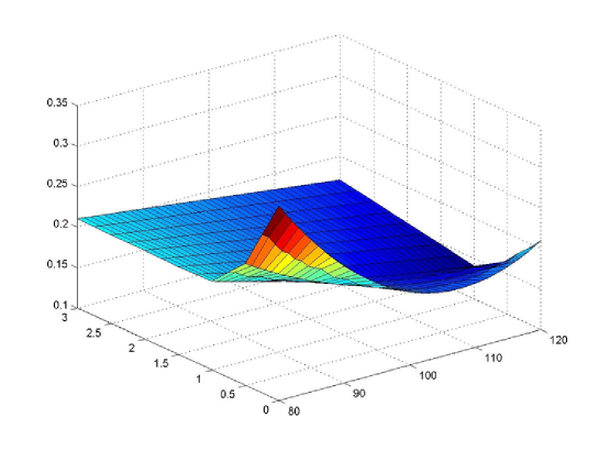
Figure 1: Implicit Volatility Surface for parameter set S1.

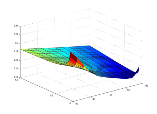
Figure 2: Implicit Volatility Surface for parameter set S2.

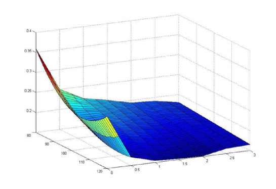
Figure 3: Implicit Volatility Surface for parameter set S3.

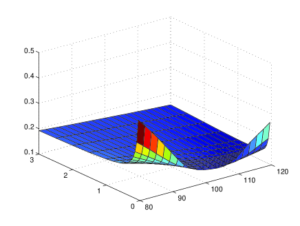
Figure 4: Implicit Volatility Surface for parameter set S4.

All the volatility surfaces obtained exhibit both smiles and skews for short maturities. While the skew is quite pronounced for the set of parameters denoted by $S_{2}$, $S_{3}$ it seems less evident for the other sets $S_{1}$, $S_{4}$. The smiles appear less and less pronounced for longer maturities for all sets. The explanation of the different behavior exhibited by the volatility surfaces seems to be related more to the different values of the diffusion coefficient $\theta$ of the volatility dynamics than to the other parameters, while the ”leverage” coefficient $\rho$ seems to be responsible of both the skews and the smiles appearing in the volatility surfaces. The behavior of the smiles in correspondence to the ”at the money values” of the call option looks moreover quite realistic.

The next two figures represent the solution obtained with the present finite element method versus the solution obtained via a Fast Fourier transform method. While the latter is represented by the continuous line, the former is indicated by the dots. The set of parameters characterizing the model are those denoted before by $S_{1}$, $S_{4}$ respectively. The range of prices is $80\leq S\leq 120$. The calculation has been performed for $T=1$, $K=100$.

A very good agreement between the solutions can be immediately recognized, although it looks quite evident that the solution obtained via the finite element method slightly overprices the call option for higher values of the underlying at time 0.

In order to check the robustness of the present method with respect to parameters changed, several trials have been performed corresponding to other sets of parameters belonging to an enlarged range of parameters and the results obtained look very close to those just presented.

The CPU time required for a calculation of the call option price for a single value of the underlying is about 3 minutes, while that required for the volatility surfaces shown here is about 3 hours on a 2Ghz Centrino Duo with 1MB RAM. The 2D mesh used in the computation is composed by 2634 triangles and 1398 nodes.

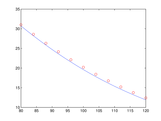
Figure 5: Comparison between the FFT solution and the FEM solution for set $S_{1}$: $T=1$ and $K=100$.

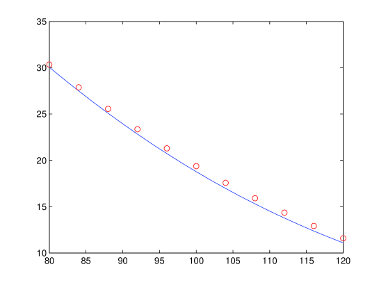
Figure 6: Comparison between the FFT solution and the FEM solution for set $S_{4}$: $T=1$ and $K=100$.

7 Concluding Remarks

We have presented a finite element approach to the european option valuation problem formulated via a partial integro-differential equation. Several choices of the functional space suitable for the spatial discretization are possible and we have made the most simple choice in order to obtain a fast and efficient algorithm. Other choices have been made by some authors in similar contexts, like in [9], [12], where Wavelets have been used in an extensive way to produce an accurate algorithm, but the convergence of the method with this choice seems to be not very fast. In the present context, with a single underlying, the choice of piece-wise polynomial function spaces seems to perform slightly better.

A natural development of the present analysis will be the variational formulation and the implementation of a finite element method for American option pricing with the Bates model. This problem can be formulated as a free boundary problem for the same Partial Integro-Differential equation given before. The finite element approach seems to be the most promising way to obtain fast and accurate algorithms for this problem. This will be the subject of future investigations.

References

- [1] Achdou, Y., Tchou, N.: Variational analysis for the Black-Scholes equation with stochastic volatility, ESAIM: Mat. Mod. and Num. Analysis, 36/3, 373-395 (2002).
- [2] Almendral, A., OOsterlee, C.W.: Numerical valuation of options with jumps in the underlying, Appl. Num. Math., 53, 1-18 (2005).
- [3] Barndorff-Nielsen, O.E., Shepard, N.: Ornstein-Uhlenbeck-based models and some of their uses in financial economics (with discussion), J. R. Stat. Soc. B, 63, 167-241 (2001).
- [4] Barndorff-Nielsen, O.E.: Modelling by Lévy processes for financial econometrics, in Lévy Processes-Theory and Applications, 283-318. Eds. O. Barndorff-Nielsen, T. Mikosch, S. Resnick, Birkauser (2001).
- [5] Bates, D.: Jumps and stochastic volatility: the exchange rate processes implicit in Deutschemark opions, Rev. Fin. Studies, 9, 69-107 (1996).
- [6] Carr, P., Madan, D.: Option valuation using the fast Fourier transform, J. of computational finance, 2, 61-73 (1998).
- [7] Cont, R., Voltchkova, E.: A Finite Difference Scheme for Option Pricing in Jump-Diffusion and Exponential Levy Models, SIAM J. Numer. Anal. 43/4, 1596-1626 (2005).
- [8] Heston, S.L.: A Closed-Form Solution for Options with Stochastic Volatility with Applications to Bond and Currency Options, Rev. Fin. Studies, 6/2, 327-343 (1993).
- [9] Hilber, N., Reich, N., Schwab, C., Winter, C.: Finite Element based derivative pricing on general price processes, Presented at Risk Day 2006, ETH Zuerich.
- [10] Hubalek, F., Sgarra, C.: Quadratic Hedging for the Bates Model, Int. Journ. of Theor. Appl. Finance, 10/5, 873-885 (2007).
- [11] Matache, A.-M., von Petersdorff, T., Schwab, C.: Fast Deterministic Pricing of Options on Lévy Driven Assets, ESAIM: Mathematical Modelling and Numerical Analysis, 38/1, 37-71 (2003).
- [12] Matache, A.-M., Nitsche, P.-A., Schwab, C.: Wavelet Galerkin Pricing of American Options on Lévy Driven Assets, Quantitative Finance, 5/4, 403-424 (2005).
- [13] Merton, R.: Option pricing when underlying stock returns are discontinuous, J. Fin. Economics, 3, 125-144 (1976).
- [14] Schoutens, W.: LEVY PROCESSES IN FINANCE, Wiley (2003).
- [15] Hilber, Matache, A.-M., Scwab, C.: Sparse wavelet methods for option pricing under stochastic volatility, J. Comp. Finance, 8/4, 1-42 (2005).
- [16] Balmisse-Thomsen, J.C.: Model Risk in pricing of Exotics, Master Thesis, Aarhus University (2006)
- [17] Cont, R., Tankov, P.: FINANCIAL MODELLING WITH JUMPS, Chapman/Hall-CRC (2004).
- [18] Carr, P., Geman, H., Madan, D., Yor, M.: Stochastic Volatility for Lévy Processes, Math. Finance, 13, 3455-382 (2003).
- [19] Venardos, E.: Derivatives Pricing and Ornstein-Uhlenbeck Type Stochastic Volatility, Ph.D. Thesis Nuffield College of Oxford (2001).
- [20] Wu, X.: Stochastic Volatility with Lévy Processes: Calibration and Pricing, Ph.D. Thesis, Dept. of Finance, University of Maryland (2005).
- [21] Zhang, X.: Analyse Numeriques des Options Américaines dans un Modèle de Diffusion avec des Sauts, Ph.D. Thesis, CERMA (1994).