The UKIRT Wide Field Camera $Z$$Y$$J$$H$$K$ Photometric System: Calibration from 2MASS

Abstract

In this paper we describe the photometric calibration of data taken with the near-infrared Wide Field Camera (WFCAM) on the United Kingdom Infrared Telescope (UKIRT). The broadband $Z$$Y$$J$$H$$K$ data are directly calibrated from 2MASS point sources which are abundant in every WFCAM pointing. We perform an analysis of spatial systematics in the photometric calibration, both inter- and intra-detector and show that these are present at up to the $\sim$5 per cent level in WFCAM. Although the causes of these systematics are not yet fully understood, a method for their removal is developed and tested. Following application of the correction procedure the photometric calibration of WFCAM is found to be accurate to $\simeq$1.5 per cent for the $J$$H$$K$ bands and 2 per cent for the $Z$$Y$ bands, meeting the survey requirements. We investigate the transformations between the 2MASS and WFCAM systems and find that the $Z$ and $Y$ calibration is sensitive to the effects of interstellar reddening for large values of $E(B-V)^{\prime}$, but that the $J$$H$$K$ filters remain largely unaffected. We measure a small correction to the WFCAM $Y$-band photometry required to place WFCAM on a Vega system, and investigate WFCAM measurements of published standard stars from the list of UKIRT faint standards. Finally we present empirically determined throughput measurements for WFCAM.

1 Introduction

This paper describes the photometric calibration of the United Kingdom Infrared Telescope (UKIRT) Wide Field Camera (WFCAM) $Z$$Y$$J$$H$$K$ passbands spanning $0.84-2.37\,\mu$m. The WFCAM photometric system, based on synthetic colours, is described in Hewett et al. (2006).

WFCAM is currently mounted on UKIRT about 75 per cent of the time, the majority of which is used to perform a set of five public surveys, under the umbrella of the UKIRT Infrared Deep Sky Survey: UKIDSS, (Lawrence et al. 2007, Warren et al. 2007), as well as a number of campaign projects and other smaller programmes.

All WFCAM data are processed and calibrated by the Cambridge Astronomical Survey Unit (CASU) using an automated pipeline (Irwin et al. 2008). Due to the large data rate of WFCAM (150–230 Gigabytes of raw image data are taken per night), a reliable and robust method for photometric calibration is required. The primary photometric calibrators are drawn from stars in the Two Micron all Sky Survey (2MASS, Skrutskie et al. 2006), present in large numbers in every WFCAM exposure (the median number is around 200 per pointing). The 2MASS calibration has been shown to be uniform across the whole sky to better than 2 per cent accuracy (Nikolaev et al. 2000).

In this paper we investigate the accuracy and homogeneity of the WFCAM calibration, by analysis of data taken in the first two years of science operations. The survey requirement is to provide a photometric calibration in broad band filters accurate to 2 per cent with a goal of 1 per cent. To test whether the calibrated photometry passes the requirements, we consider the following tests:

• for repeat observations of non-variable stars (of sufficient signal-to-noise), the measured $rms$ (root mean square) should be no worse than 0.02 magnitudes.

• the calibration should be robust against the effects of reddening, i.e. the calibrated frame zeropoints, measured on photometric nights, should have a standard deviation $\leq 0.02$ magnitudes as a function of reddening.

• the photometric calibration should be uniform across the sky, and not depend on the observed stellar population or the number of stars in the image. Specifically, the calibrated frame zeropoints (on photometric nights) should have a 1$\sigma$ scatter of $\leq 0.02$ magnitudes even in sparse regions of sky, e.g. at high Galactic latitude.

We demonstrate that for the vast majority of observations with WFCAM, these tests are passed, and we quantify the conditions under which they are not.

The paper is organised as follows: Section 2 summarises how the WFCAM data are calibrated within the pipeline; in Section 3 we examine the repeatability of WFCAM photometry, quantify residual spatial systematics, and investigate the limits of the calibration in non-photometric conditions; in Section 4 we investigate the relationship between the 2MASS and WFCAM photometric systems and investigate the effects of interstellar reddening; in Section 5 we investigate the extent of bias in the WFCAM calibration arising from the overestimation of flux in faint sources in 2MASS; in Section 6 we compare the WFCAM system to a Vega system where A0 stars should have zero colour in all passbands; in Section 7 we compare the WFCAM photometry with published data for faint standards measured with UKIRT; Finally, in Section 8 we derive the throughput of WFCAM. At the time of writing, UKIDSS has completed its fourth Data Release (DR4).

2 Method for routine photometric calibration of WFCAM data

All WFCAM data are processed in Cambridge with a pipeline developed by CASU and documented in Irwin et al. (2008). In this section we describe in detail the steps used to measure magnitudes and then apply a photometric calibration for each WFCAM image and subsequent catalogue. After processing and calibration, the WFCAM data (in the form of FITS binary images and catalogues) are transferred to Edinburgh for ingestion into the WFCAM Science Archive (WSA, Hambly et al. 2008). The UKIDSS data have now seen a number of data releases from the WSA, and the photometric calibration has evolved to tackle the (increasingly smaller) corrections needed to meet the survey goals; the corrections included in each release are summarised in Table 1.

Table 1: Summary of photometric calibration corrections included in each UKIDSS release from the WSA. The columns indicate which of the following are accounted for: a reddening dependent correction (see Section 4.3), a per-chip zeropoint (discussed in Section 2.3), a radial distortion term (Section 2.2), and a residual 2D spatial systematic correction (Section 3.2.3).

Release	Date	E(B-V)’	chip ZP	radial	spatial
EDR	Feb 2006	no	no	no	no
DR1	Jul 2006	no	no	no	no
DR2	Mar 2007	yes	no	no	no
DR3	Dec 2007	yes	yes	no	no
DR4	Jul 2008	yes	yes	yes	yes

2.1 Key WFCAM elements

WFCAM comprises four Rockwell Hawaii-II PACE arrays, with 2k $\times$ 2k pixels at 0.4 arcsec/pixel, giving a solid angle of 0.21 deg² per exposure. A detailed description of WFCAM can be found in Casali et al. (2007). A prerequisite for the calibration scheme is to ensure that all four detectors are calibrated to the same photometric system. The implementation of the reduction pipeline needs to ensure that the different intrinsic detector quantum efficiencies (and possibly their different colour dependence) are correctly taken into account. Thus much of the calibration is performed per-detector.

There are five broadband filters designed for WFCAM, the $Z$$Y$$J$$H$$K$ filters, which are described in detail by Hewett et al. (2006) and characterized using synthetic photometry. The $J$$H$$K$ filters possess transmission profiles specified to reproduce as closely as possible the widely adopted MKO system (Tokunaga, Simons & Vacca 2005). The $Z$ and $Y$ filters cover 0.84–0.93$\mu$m and 0.97–1.07$\mu$m respectively.

2.2 Measurement of instrumental magnitudes

The source extraction software (Irwin et al. 2008) measures an array of background-subtracted aperture fluxes for each detected source, using 13 soft-edged circular apertures of radius $r/2$, $r/\sqrt{2}$, $r$, $\sqrt{2}r$, $2r$ … up to $12r$, where $r=1$ arcsecond. A soft-edged aperture divides the flux in pixels lying across the aperture boundary in proportion to the pixel area enclosed. In this paper we only consider photometry derived from fluxes measured within an aperture of radius 1 arcsecond. However, all the apertures of selected isolated bright stars are used to determine the curve-of-growth of the aperture fluxes, i.e. the enclosed counts as a function of radius. This curve of growth is used to measure the point spread function (PSF) aperture correction for point sources for each detector, for each aperture (up to and including $4r$, which includes typically $\sim$99 per cent, or more, of the total stellar flux). Irwin et al. (2008) find that this method derives aperture corrections which contribute $\leq 1$ per cent to the overall photometry error budget

A further correction should be applied to the source flux to account for the non-negligible field distortion in WFCAM, described in detail in Irwin et al. (2008). The astrometric distortion is radial and leads to an increase in pixel area by around 1.2 per cent compared to the centre of the field of view. Standard image processing techniques assume a uniform pixel scale, and that a correctly reduced image will have a flat background. For WFCAM’s variable pixel scale, this is actually incorrect and one would expect to see an increase in the sky counts per pixel at large off-axis angles, while the total number of counts detected from a star would be independent of its position on the array. The flatfielding of an image therefore introduces a systematic error into the photometry of sources towards the edge of the field of view. The corrected flux $f_{\rm cor}$, where $f$ is defined as the aperture corrected count-rate in ADU per second of the source above background, is simply:

$$f_{\rm cor}=f/(1+3k_{3}r^{2})(1+k_{3}r^{2})$$ (1)

Where $k_{3}$ (with units of radian/radian³) is the coefficient of the third order polynomial term in the radial distortion equation (Irwin et al. 2008) and is found to be slowly wavelength dependent with a value of -50.0 in the $H$-band (called PV2_3 in the FITS headers). The instrumental magnitude is then

$$m_{i}=-2.5log_{10}(f_{\rm cor})$$ (2)

This correction has not been applied for WSA releases DR1–DR3 (Hambly et al. 2008), but is included for DR4 and subsequent releases. Fig. 1 plots the radial distortion term ($f_{\rm cor}/f$ converted to magnitudes) as a function of off-axis angle for the WFCAM filters.

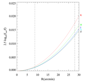
Figure 1: Photometric radial distortion (magnitudes) in WFCAM as a function of offaxis angle (arcmin). There are curves for all five broadband filters, $Z$$Y$$J$$H$$K$ from bottom to top. The WFCAM detectors are separated by 94 per cent of their active area in a square pattern (see Fig. 4), thus the vertical lines represent the location of the detector corners.

2.3 Calibration of the photometry

The data are firstly flatfielded using twilight flatfields (which are updated monthly), and an initial gain correction is applied to place all four detectors on a common system, to first order. The per-detector magnitude ZP is then derived for each frame from measurements of stars in the 2MASS point source catalogue (PSC) that fall within the same frame. Thus the calibration stars are measured at the same time as the target sources, taking us away from more traditional calibration schemes, whereby standard star observations are interspersed with target observations.

We assume that there exists a simple linear relation between the stellar 2MASS and WFCAM colours, e.g. $J_{\rm w}-J_{2}\propto J_{2}-H_{2}$. In a Vega-based photometric system, this relation should pass through (0,0), i.e. for an A0 star $Z$ = $Y$ = $J$ = $H$ = $K$, irrespective of the filter system in use. For each star in 2MASS observed with WFCAM, the pipeline derives a ZP (at airmass unity) from

$$ZP=m_{\rm 2}+C(J_{2}-H_{2}\,{\rm or}\,J_{2}-K_{2})-m_{i}+k(\chi-1)$$ (3)

where $m_{i}$ is the aperture corrected instrumental magnitude (derived above). $C$ are the colour coefficients for each passband and have been solved for by combining data from many nights (see Section 4). $k$ is a default value for the extinction (0.05 in all filters, see below) and $\chi$ is the airmass.

The 2MASS sources used for the calibration of WFCAM are selected to have extinction-corrected colour $0.0\leq J_{2}-K_{2}\leq 1.0$ with a 2MASS signal-to-noise ratio $>10$ in each filter. If fewer than 25 2MASS sources are found within the field-of-view of the detector, then the colour cut is not applied. The WFCAM astrometric calibration is also derived from 2MASS and for both systems the astrometric $rms$ accuracy per source is $<$ 100mas (Irwin et al. 2008). The maximum allowed separation for a 2MASS-WFCAM source match is 1 arcsecond. For all WFCAM observations up until 2008 March 28th, the median number of 2MASS stars falling within a WFCAM detector, which match our colour and signal-to-noise requirements, is $\sim 200$. Only around 0.1 per cent of WFCAM pointings have fewer than 25 2MASS stars covering a single detector. For the UKIDSS Large Area Survey (LAS) alone, the median number of 2MASS standards per detector is $\sim 100$, and again, around 0.1 per cent have fewer than 25.

For a single pointing, for each detector, the zeropoint is then derived as the median of all the per-star zeropoint values. A single photometric zeropoint for the pointing, MAGZPT, is calculated as the median of the detector zeropoints over all 4 detectors. The associated error, MAGZRR, is 1.48$\times$ the median absolute deviation of the detector zeropoints around the median. This error therefore comprises several components: the intrinsic errors in the 2MASS photometry, the error in the conversion from 2MASS to the WFCAM filter, and then any residual systematic offsets between the detectors (see Section 3.2.2). In the $Z$-band, the MAGZRR errors are the largest, typically about twice that for the $J$$H$$K$ filters.

It should be noted that we do not derive any atmospheric extinction terms on a given night with WFCAM. Rather, the value of MAGZPT derived above incorporates an instantaneous measure of extinction at the observed airmass. The photometric calibration of a field therefore includes no error from this assumption. However the derived zeropoint for airmass unity will include a small error (because we assume the extinction is 0.05 magnitudes per airmass for all filters). Leggett et al. (2006) find the extinction at Mauna Kea to be $k_{J}=0.047$, $k_{H}=0.029$, $k_{K}=0.052$ with standard deviations between 0.2 and 0.3. For a typical WFCAM frame, observed at an airmass$\approx 1.3$, an extinction which differs from our assumed value by 0.03 magnitude/airmass will lead to a 0.01 magnitude error in the value of MAGZPT. The value of MAGZPT over time can be used to investigate the long term sensitivity of WFCAM due to, for example, the accumulation of dust on the optical surfaces, and seasonal variations in extinction.

2.4 Detector offsets

A final stage to the photometric calibration takes account of systematic differences between the four detectors, measured on a monthly basis. The object catalogues associated with each science product frame are used in the pipeline calibration process to compute a single per pointing overall zeropoint for the array of 4 detectors, using the colour equations specified in Section 4. The residuals from all 2MASS stars used in the frame zeropoint determination (i.e. $J$, $H$, $K$ signal:noise $>$ 10:1) are also computed on a per pointing basis together with their standard coordinate location ($\xi,\eta$) with respect to the tangent point of the telescope optical axis (see e.g. Irwin et al. 2008). We use standard coordinates since these are independent of the degree of interleaving and dithering, and hence pixel scales, used in constructing the science product images and catalogues. These residuals are then partitioned by month and stacked. The monthly timescale corresponds with the changover of the master flat field frames, with which we anticipate some of the corrections are correlated. From UKIDSS DR3, all WFCAM photometric calibration is determined and applied monthly. The details of this correction process are discussed in Section 3.2.1. The result is to generate zeropoints per detector (the value of MAGZPT is updated for each detector).

The pipeline also estimates the nightly zeropoint (NIGHTZPT) and an associated error (NIGHTZRR) which can be used to gauge the photometricity of a night. NIGHTZPT is simply the median of all ZPs measured within the night, and NIGHTZRR is a measure of the scatter in NIGHTZPT.

3 Repeatability of the photometry

3.1 Overlap analysis from the UKIDSS Large Area Survey

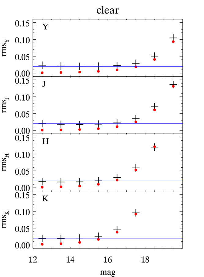
Figure 2: $rms$ diagram for repeat observations of sources in the DR3 dataset for the LAS (selected to be stellar in both observations) for the $Y$$J$$H$$K$ filters (top to bottom), showing results for data taken in photometric conditions. Photometric conditions are defined as having a zeropoint within 0.05 magnitudes of the survey median value. Black crosses are 1.48 $\times$ the MAD (median absolute deviation) of the data in magnitude slices, i.e. equivalent to the Gaussian sigma of the magnitude bin. Red circles are the median pipeline errors for sources in the bin as reported in the WFCAM Science Archive for DR3. The blue horizontal lines at 0.02 magnitudes represent the target 2 per cent photometric reliability.

We can use repeat observations of sources in UKIDSS to investigate the photometric accuracy and homogeneity of the survey and to compare with the pipeline errors. The pipeline errors are calculated from the source counts and local background only, and do not include corrections for bad pixels and other detector artifacts. In addition, they deliberately do not include any contribution from the calibration procedure itself (i.e. the inherent uncertainties in the calibrators) or additional corrections for residual systematic effects in the calibration. By comparing multiple observations of sources near the edges of the detectors we are more sensitive to systematics from spatial effects, e.g. scattered light in the flatfield, a variable point spread function, and so on (see Section 3.2). Hence this analysis demonstrates the worst case, and should help put upper limits on the error contribution from systematic contributions.

Fig. 2 shows the $rms$ diagrams for repeat measurements, for all point sources (classed as stellar in both observations) in the DR3 release of the LAS. Repeat observations arise from the small overlap of detector edges between the four pointings which go towards constructing a tile, as well as from observations of adjacent tiles. The $rms$ for each magnitude bin is calculated from the standard deviation of the differences between the two measurements from all the repeats, $\sigma_{\Delta mag}/\sqrt{2}$. The data used in Fig. 2 were observed in photometric conditions, with a frame photometric zeropoint within 0.05 magnitudes of the median value for all observations made with the filter ($\sigma_{\rm ZP}=0.03$ magnitudes in all pass bands). We exclude sources at the very edges of the array, within 10 arcseconds of the detector edges.

For a photometric calibration good to 2 per cent, then the median magnitude difference should be zero, and the $rms$ of the distribution for the brighter stars should be $\sigma/\sqrt{2}=0.02$.

At the bright end, the $rms$ (black crosses in Fig. 2) is very close to the survey goal of 2 per cent. Unsurprisingly, the pipeline estimated random noise errors (red dots in Fig. 2) significantly underpredict the observed distribution at the bright end, indicating that systematic errors, dominate here at the 2 per cent level. Figure 3 combines measurements for all filters and compares the estimated random photon noise errors, $E$, derived by the pipeline to the measured errors $M$ (the $rms$ described above), which include both systematic calibration errors and random components due to photon noise. The points have been fitted with a simple relation of the form $M^{2}=cE^{2}+s^{2}$ where the systematic component $s=0.021\pm 0.001$, the constant of proportionality $c=1.082\pm 0.014$. In principle these can be used to update the default pipeline error estimates, however, we suspect that $c$ is slightly greater than unity due to a combination of factors relating to edge effects on the detectors and noise covariance arising from inter-pixel capacitance within the detector (Irwin et al. 2008), which the pipeline error estimates do not allow for.

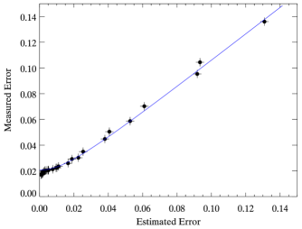
Figure 3: A plot of measured errors ($M$) against estimated errors ($E$) derived from the $rms$ distributions for LAS overlaps. The solid line is a linear fit to $M^{2}$ versus $E^{2}$ and is described in the text.

3.2 Spatial systematics

3.2.1 Measurement

As described in Section 2.3, we store the standard coordinates ($\xi,\eta$) and WFCAM magnitude for each observation of a 2MASS star. For each month of data and for each filter we then compute a per star zeropoint relative to the previously computed overall zeropoint for each science product image for the entire array. These differences are then stacked within a fixed standard coordinate grid, of cell size $\approx 1.2\times 1.2$ arcmin covering the complete array of four detectors, making use of selected data from each month of observations. Only science products taken in photometric conditions are used in this process to minimise the effects of non-photometric residual structure. The average offsets in the grid of values are then filtered (smoothed) using a combination of a two-dimensional 3-pixel bimedian and bilinear filter. This latter step ensures a smooth variation of values over the grid by effectively correlating the corrections on a scale of neighbouring grid points. This is necessary since, even with a month of data, the number of points per cell is still only typically 25-100. The $rms$ noise per cell from the 2MASS errors alone is $\approx$1 per cent. With smoothing, this noise drops to the few milli-mag level which is a negligible extra error with respect to the derived corrections.

The residuals for each detector are then grouped and the median correction calculated. These median factors define the detector-level zeropoint corrections for each passband. The final stage is to apply the detector-level corrections and compute the residual systematics which are recorded as a correction table, and diagnostic plot. An example of the latter is shown in Fig. 4 and the possible origins of these patterns are discussed below. The correction tables are currently available via the CASU web pages.

Figure 4: An example of the remaining monthly average spatial magnitude residuals for WFCAM $J$-band observations in 2005 September after applying passband-dependent individual detector zeropoint corrections. The residuals are shown in standard coordinates with respect to the tangent point of the observations, i.e. E is to to the left and N is to the top.

3.2.2 Detector-to-detector offsets

The detector zeropoint level corrections show some interesting effects when data from five WFCAM semesters are examined (see Fig. 5). The small random jumps in the temporal sequences are most likely due to detector-level DC offsets caused by flatfield pedestal effects (these can also be seen in the sky corrections but in this case they are generally additive and do not impact object photometry). Additionally, $\approx\pm$1 per cent, more constant trends are seen in the offsets. These are correlated within a passband but are different between bands.

We wondered if small QE variations between the detectors could give rise to slightly different colour equations, required to relate the natural detector+filter+telescope passband to the 2MASS standards. The overall passband gain differences between the detectors are corrected at the flatfielding stage but because the twilight sky used in the flats is generally a different colour from the majority of objects, residual colour equation differences between the detectors could be manifest as a small zeropoint offset. Analysis of WFCAM images shows that the twilight sky changes colour rather rapidly as the sky darkens, ranging from fairly neutral ($J-K\sim 0.5$), through extremely blue ($J-K\sim-2.0$), to the rather red dark sky ($J-K\sim 2.5$). Modelling of the twilight sky and typical calibration stars (using a range of synthetic spectra as input) suggest that the detectors would have to exhibit large differences in QE, at the 10 per cent level, across individual passbands to explain the observed effect. Hewett et al. (2006) found that the QE of a typical Rockwell Hawaii-II detector increases approximately linearly with wavelength, by 8 per cent over the entire WFCAM 0.8–2.2 micron range. However we currently lack measurements of the actual WFCAM detector QEs. For the time being, the cause of the detector-to-detector photometric offsets remains an open question.

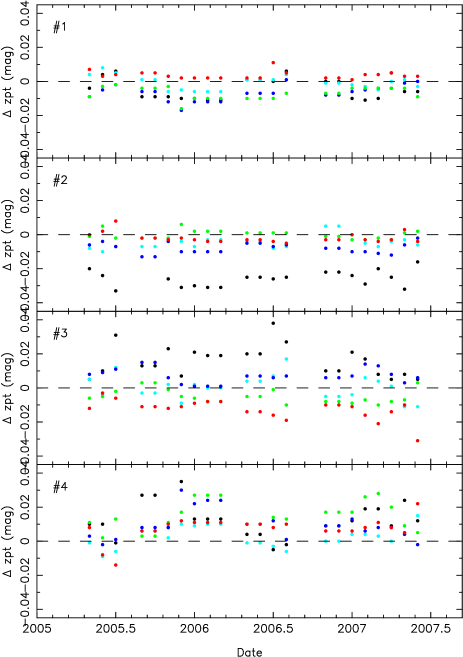
Figure 5: An overview of the computed detector zeropoint corrections as a function of observation date for all of the WFCAM broadband filters: $Z$ - black; $Y$ - cyan; $J$ - blue; $H$ - green; $K$ - red. The patterns broadly split into a constant offset component, and occasional random jumps in level believed to be caused by DC pedestal level offsets in the derived flatfield frames. The numeric label on each panel refers to the detector with #1 SW, #2 SE, #3 NE, #4 NW as seen on the sky.

3.2.3 Residual spatial systematics and their possible causes

After removing the detector-level differences, generic recurring patterns are visible in the final spatial correction, even across different passbands. This strongly suggests a common underlying cause and the three most likely contributors are:

1. spatially dependent PSF corrections – the residual maps are made from aperture-corrected 2 arcsec diameter flux measurements.

2. low-level non-linearity in the detectors;

3. scattered light in the camera which would negate the implicit assumption of, on average, uniform illumination of the field;

We have ruled out spatial PSF distortions as a significant contributor by comparing aperture-corrected 4 arcsec diameter fluxes with the 2 arcsec diameter measures. If we exclude observations made in the first 4 months of WFCAM operations, when adjustments to the focal plane geometry were still being made, the average systematic difference between 2 and 4 arcsec diameter stellar fluxes is negligible ($<$1 per cent) over the entire array.

3.2.4 Residual non-linearities?

The spatial magnitude residuals are generally larger toward the edges of the chips. To test the derived lookup tables, we repeated the LAS overlap analysis (Section 3.1), but this time after correcting the source photometry. To apply the corrections we used bilinear interpolation to compute the offset for each source in the standard coordinate system described above. The correction is applied additively.

The resulting $rms$-diagram (Fig. 6) shows a significant improvement compared to the version without spatial correction (Fig. 2). The median values of $rms$ for bright stars (taking the mag=13.5 bin in all filters), in each passband are typically 0.002-0.004 magnitudes lower (Table 2).

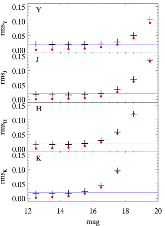
Figure 6: $rms$ diagram for repeat observations of sources in the DR3 dataset for the LAS (selected to be stellar in both observations) for the $Y$$J$$H$$K$ filters (top to bottom), after correcting for the spatial systematics as described in the text. Data are for photometric conditions only. Black crosses are 1.48 $\times$ the MAD (median absolute deviation) of the data in magnitude slices, i.e. equivalent to the Gaussian sigma of the magnitude bin. Red circles are the median pipeline errors for sources in the bin as reported in the WSA for DR3. The blue horizontal lines at 0.02 magnitudes represent the target 2 per cent photometric reliability.

We can try to gain some insight into the cause of the spatial systematics by looking at the dependence of the correction on magnitude. This would show up any residual non-linearity effects for example. In Fig. 7 we plot the quadrature difference between the spatially corrected and non-corrected $rms$ as a function of magnitude, i.e. the error contribution from the spatial systematics. We show the diagram for stars as well as galaxies, as any non-linearity effects would be less pronounced in spatially extended sources. Fig. 7 shows that the spatial systematics amount to a correction of about 1 per cent in all filters with no dependence on magnitude. We conclude that the WFCAM system shows no significant residual non-linearity. Our conclusion is consistent with the analysis of Irwin et al. (2008) who show WFCAM is linear to at least 1 per cent.

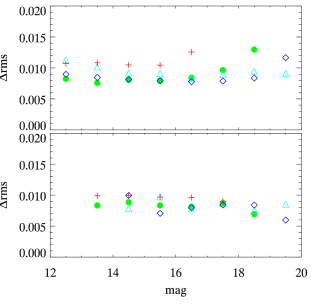
Figure 7: $\Delta rms$ is equal to $\sqrt{(}rms^{2}-rms_{\rm spatial}^{2})$ and is plotted against magnitude for the $Y$ (cyan triangle), $J$ (blue diamond), $H$ (green filled circle) and $K$ (red plus) filters. In the upper panel we plot the data for objects classified as stellar, while the lower panel is for extended sources. $rms$ is the $rms$ for photometry in the DR3 release of the LAS (as described in Fig. 2). $rms_{\rm spatial}$ is the $rms$ for the same data but with photometry corrected for spatial systematics as described in the text.

3.2.5 Scattered light as a cause of the spatial systematics?

Fig. 8 shows the correlation between normalised flatfield level and the spatial magnitude residuals for $J$-band data analysed from 2005 September. The detectors with the largest and smallest flatfield variations (#1 and #4) show no effects at the $\mathrel{\hbox{\hbox to0.0pt{\hbox{\lower 4.0pt\hbox{$\sim$}}\hss}\hbox{$<$}}}$1 per cent level; whereas detectors #2 and #3 show a clear correlation between residual magnitude spatial systematics and flatfield level. The spatial variation in the flatfield intensity is dominated by changes in sensitivity across the detectors (and vignetting within the optical train) and reaches a factor two for the worst detector (Irwin et al. 2008). The spatial systematics seen in the stacked 2MASS photometric residuals represent a 1 per cent error contribution, and it seems most likely to arise from (as yet unquantified) scattered light within the WFCAM system, probably present in all observations.

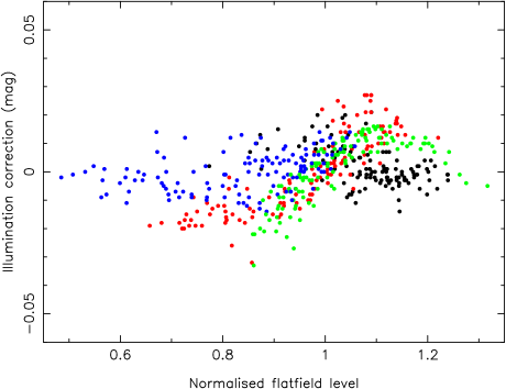
Figure 8: The correlation between normalised flatfield level and the spatial magnitude residuals for $J$-band data from 2005 September. Detectors #1 (black) and #4 (blue) show no strong correlation, however detectors #2 (red) and #3 show a well-defined correlation.

3.3 Repeat observations of standard fields

Standard star fields are observed every night with WFCAM, and provide another means of testing the repeatability of the photometric calibration. For this analysis we made use of data calibrated for UKIDSS DR3. Twenty-seven standard reference fields were selected and, for each field, reference stars were chosen to have a minimum of 100 detected counts in a 2 arcsecond diameter aperture. Fields typically contain between 500 and 10,000 suitable reference stars depending on Galactic latitude. The reference stars were then matched against subsequent observations of the same fields taken in good conditions (i.e. the frames pass the following criteria: seeing $\leq 1.52$ arcseconds, airmass $\leq 1.8$, NIGHTZRR $\leq 0.05$, MAGZRR $\leq 0.05$, median source ellipticity $<0.2$). On average, the reference fields have between 20 (in the $Z$-band) and 50 (in the $K$-band) observations which match our criteria. The smaller number of selected $Z$-band observations is due to the larger error in the frame zeropoints (Section 2).

For the repeat observations of the standard fields, the same 2MASS calibrators are used in each observation, thus we should expect to see an improvement in $rms$. The actual median values for $rms_{\rm STD}$ (for the 13.5 magnitude bin) range from 0.011–0.015 magnitudes for bright stars, which are 0.004–0.006 magnitudes lower than the spatially corrected LAS $rms_{\rm spatial}$.

3.4 Calibration performance for data taken in non-photometric conditions

The measured zeropoint for each frame depends directly on the transmission of the atmosphere. The presence of clouds leads to a reduction in the derived zeropoint. In Fig. 9 we investigate the $rms$ for stars measured in different conditions to investigate whether there is a specific sky transparency beyond which the photometric conditions become unacceptable. We again compute the $rms$ for magnitude differences between repeat measurements, but this time over a larger magnitude range, m=12–15 in all filters (it’s clear from Fig. 2 that the $rms$ in this magnitude range is largely dominated by systematic errors over photon counting). The data are plotted as a function of sky extinction as measured by the difference of the frame zeropoint from the median zeropoint for that filter for at least one of the frames (except for the ’clear’ sky case, where both frames must have an extinction $\leq 0.05$mag.

Fig. 9 demonstrates that, even in non-photometric conditions, where 10–20 per cent of the stellar flux is lost to cloud, the calibration is still very good, and still meets the 2 per cent calibration requirements.

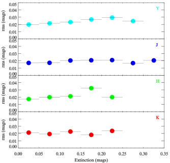
Figure 9: $rms$ as a function of sky extinction for stars with magitudes in the range 12–15. The sample is drawn from the LAS DR3 and the $rms$ values for each bin are computed from the magnitude differences between repeat observations of the same star, see Fig. 2 for details. At least one of the frames in each pair must have an extinction value in the range plotted (except for the best weather bins, which must have both frames taken with a ZP within 0.05 mags of nominal). The data are plotted by filter, $YJHK$ from top to bottom.

3.5 Photometric repeatability: summary

In Table 2 we tabulate the $rms$ at mag=13.5, for each filter, for the different samples considered in the sections above. Examining the first three columns, the largest calibration improvement comes from the computation of a per-detector zeropoint, as included in the change to WFCAM processing for DR3 from DR2. The overlap analysis of the LAS DR3 data shows that the calibration requirements for WFCAM are met, and that the photometry is repeatable to $\simeq$2 per cent, even for sources which are close to the edge of the field of view, where residual systematics are larger. Investigation of these systematics suggests that they are most likely caused by scattered light present in the WFCAM flatfields, which contributes about 1 per cent to the overall photometric error budget at large off-axis angles. Application of our corrections for these systematic residuals reduces the WFCAM photometric error to only $\simeq$1.5 per cent in $J$, $H$ and $K$.

Repeat measurements of standard fields, where the sources are uniformly distributed across the field of view, and the 2MASS calibrators do not change yield a photometric repeatability at the level of 1–1.5 per cent.

Even observations taken through thin cloud (where transmission is $>$ 80 per cent) can be calibrated to $\simeq$2 per cent using 2MASS stellar sources as secondary standards.

Table 2: $rms$ at mag=13.5 for the WFCAM filters derived from repeat observations of sources in the LAS and standard star fields.

	LAS				STD
Filter	$rms_{\rm DR2}$	$rms_{\rm DR3}$	$rms_{\rm spatial}$	$rms_{\rm cloudy}$	$rms_{\rm STD}$
$Z_{\rm w}$	-	-	-	-	0.015
$Y_{\rm w}$	0.023	0.021	0.019	0.021	0.013
$J_{\rm w}$	0.021	0.018	0.016	0.022	0.012
$H_{\rm w}$	0.022	0.017	0.015	0.021	0.011
$K_{\rm w}$	0.023	0.020	0.016	0.020	0.011

4 Comparison between WFCAM and 2MASS photometric systems

The colour equations determined for regions of low reddening are listed below. They were derived from fits to selected data taken in the first year of WFCAM observations (Irwin et al. 2008). The 0.03 magnitude offset for the $H$-band is discussed below. The $Y$-band offset was not included prior to DR3, and is discussed in Section 6.2. In this Section we rederive the 2MASS–WFCAM tranformations, and investigate their behaviour in regions of low and high Galactic latitude. We establish the reliability of the photometry for fields containing relatively small numbers of 2MASS calibrators. We also quantify the effects of Galactic extinction on the calibration, and derive additional corrections for Equations 4–8, listed in Equations 9–13. For DR2 onwards, it is this full set of equations that are applied to the 2MASS secondary standards to enable derivation of the photometric zeropoint.

$$Z_{\rm w}=J_{2}+0.950(J_{2}-H_{2})$$ (4)

$$Y_{\rm w}=J_{2}+0.500(J_{2}-H_{2})+0.080$$ (5)

$$J_{\rm w}=J_{2}-0.065(J_{2}-H_{2})$$ (6)

$$H_{\rm w}=H_{2}+0.070(J_{2}-H_{2})-0.030$$ (7)

$$K_{\rm w}=K_{2}+0.010(J_{2}-K_{2})$$ (8)

4.1 The 2MASS colour-terms

Fig. 10 shows data derived from observations taken in the second half of 2005. We plot the difference between the calibrated WFCAM photometry and the 2MASS photometry for some 200,000 measurements across five passbands. We use these data to rederive the colour-terms to compare to those in Equations 4–8. The data are selected to avoid regions of high interstellar reddening, $E(B-V)^{\prime}$

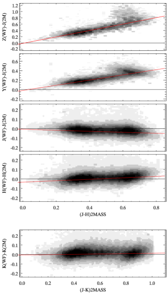
Figure 10: A Hess diagram showing differences between WFCAM and 2MASS photometry as a function of 2MASS ($J_{2}-H_{2}$ or $J_{2}-K_{2}$) colour for data taken in the second half of 2005. The data have been selected such that $E(B-V)^{\prime}\leq 0.2$ and $J_{2}-K_{2}\leq 2.0$ to avoid the most significant effects of reddening. The best fit linear regressions to the unbinned data are overplotted.

The data are fit with a linear relation (with 3$\sigma$ clipping), including only stars with colours in the range $0.0\leq J_{2}-K_{2}\leq 1.0$. The slopes of the fits for are shown in Fig. 10 and can be seen to be in good agreement with Equations  4 to 8.

Table 3: Table of best fit colour terms for WFCAM–2MASS colour as a function of $J_{2}-H_{2}$ (or $J_{2}-K_{2}$ in the case of the K filter) as shown in Fig. 10, split by region (see text for details). The first column shows the best fit colour terms for data taken in the second half of 2005 (semester 05B) and can be directly compared to the colour equations listed in Equations 4 to 8.

	Semester	Region
Colour	05B	A	B	C
$Z_{\rm w}-J_{2}$	1.02	1.04	0.92	1.01
$Y_{\rm w}-J_{2}$	0.55	0.51	0.55	0.56
$J_{\rm w}-J_{2}$	-0.05	-0.04	-0.06	-0.05
$H_{\rm w}-H_{2}$	0.08	0.04	0.07	0.07
$K_{\rm w}-K_{2}$	0.02	0.01	0.01	0.01

For the $J$$H$$K$ passbands, the linear conversions work surprisingly well, given the large spread in Figure 10. For the $H$-band, an additional 3 per cent offset is required to bring the WFCAM photometry onto the same system as the UKIRT faint standards (as originally published by Hawarden et al. 2001). The $H$-band offset is discussed in more detail in Section 7.

For the $Z$ and $Y$ passbands, significant (and indeed degenerate) residuals are seen for stars with $J_{2}-H_{2}\sim$ 0.5—0.7. This is most easily understood by appealing to the two-colour $J-H$ vs. $H-K$ diagram for dwarf stars, e.g. Fig. 2 in Cruz et al. (2003). Stars with spectral types later than M0 become progressively bluer in $J-H$, but redder in $Z-J$ and $Y-J$. Thus the same colour transformation is applied to stars with the same $J-H$ colours but very different temperatures and therefore $Z-J$ colours, resulting in the structures seen in Fig. 10.

The formal errors on all the fits are extremely small due to the large numbers of sources present in each sample, and are not particularly helpful when considering that they do not account for systematic effects (e.g. population). Below we consider two issues: (1) how robust is the determination of zeropoint assuming the colour equations are correct for randomly selected small samples of stars, matched to the example of the Large Area Survey?; (2) are the colour equations significantly different in regions of high and low Galactic latitude?

4.2 Robustness of zeropoint determination

For the determination of the zeropoint of a typical high-latitude field, the measured offset between the WFCAM instrumental magnitudes and the 2MASS photometry will not be affected by these colour-dependent residuals, so long as a robust (i.e. median) offset is measured. Clearly the average offset in the top two panels in Fig. 10 would be affected by the non-linearity in the colour-transformations. If a WFCAM field were dominated by extremely red stars, or an unusual population of objects (for example a large and rich Globular Cluster), then a further colour-dependent zeropoint correction may be necessary. We have yet to identify any fields that suffer from this effect. For example, examining zero-point variation as a function of Galactic latitude and longitude reveals no compelling evidence for any variation significanlty larger than 1 per cent. We anticipate returning to this issue in the future as more data are collected over larger areas of sky.

The robustness of the calibration of WFCAM is most simply tested using a Monte-Carlo approach. We took a ‘worst-case’ scenario, comprising a high-latitude field which contains relatively few 2MASS stars. For each trial we selected 50 stars at random (from the dataset used above), and derived the median offset between the 2MASS magnitudes corrected to the WFCAM system (using Equations 4–8) and the WFCAM calibrated photometry. We performed 10,000 trials, and summarise the results in Table 4. This method of calibration is found to be robust for all filters, with a standard deviation of 1 per cent or lower in all filters, except the $Z$-band, for which the error is closer to 2 per cent.

Table 4: Average Zeropoint offsets and their standard deviations for a comparison between the 2MASS and WFCAM photometry for 10000 trials with randomly chosen samples of 50 stars

Filter	Mean ZP Offset	$\sigma_{\rm offset}$
$Z_{\rm w}$	-0.006	0.017
$Y_{\rm w}$	-0.001	0.011
$J_{\rm w}$	0.003	0.007
$H_{\rm w}$	0.002	0.008
$K_{\rm w}$	0.003	0.010

4.2.1 Colour equations at low and high Galactic latitude

We defined three regions to compare: A ($0<l<100$, $|b|<10$), B ($0<l<100$, $|b|>20$), C ($180<l<250$, $|b|>15$), where $l$ and $b$ are Galactic longitude and latitude respectively. Region A thus contains a fairly large sample close to the Galactic plane. As with the sample examined above, we fit for the colour transformations between the 2MASS and WFCAM filters. The results of the fitting are listed in Table 3. There appear to be some small differences between the regions, particularly in the Z-passband for region B. However, bootstrap error estimates find an error in the slope of $\pm 0.02$ for regions B and C in this filter, so we do not believe these differences to be significant (above 2$\sigma$). Note that the colour term for a pointing would need to be adjusted by 0.04 to change the zeropoint by 2 per cent for stars of median $J_{2}-H_{2}=0.5$.

4.3 The Effects of Galactic extinction

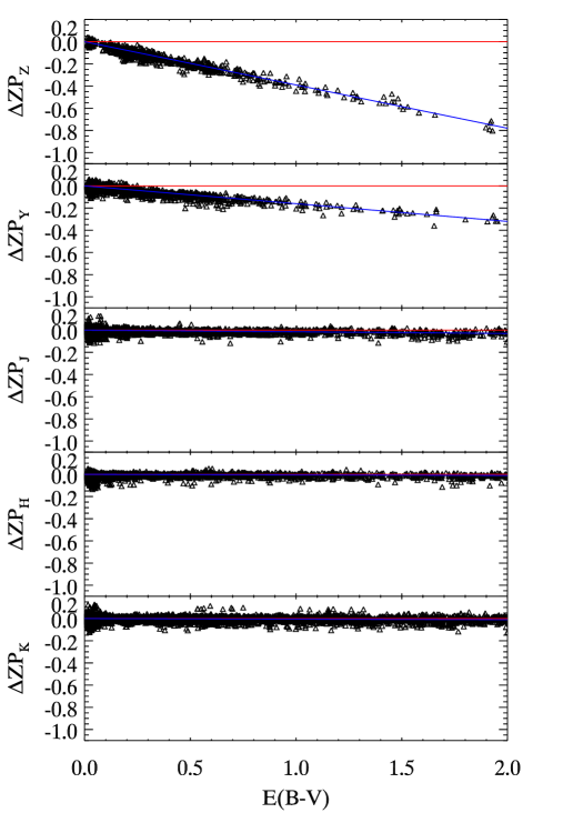
Figure 11: Frame zeropoint minus nightly zeropoint (uncorrected for reddening) versus $E(B-V)^{\prime}$ for the WFCAM broadband filters. Only data from photometric nights are included. Data points which lie more than 0.1 magnitudes away from the fit are clipped. The blue line is the best fit relation to the extinction relation, while the red line is constant $\rm\Delta ZP=0.0$.

We have attempted to mitigate against the effects of interstellar reddening on the WFCAM calibration by employing a colour restriction to the stars used in the calibration (applied after extinction correction). At regions of low Galactic latitude, where reddening is high, the spectra of distant stars are strongly affected by intervening dust. The population mix of the WFCAM calibrators will change as intrinsically blue stars are moved into the applied colour selection, and redder stars are moved beyond the colour bounds. Giant stars become significantly more common. Differences between the WFCAM and 2MASS filter profiles become important, and the colour equations used to transform the 2MASS magnitudes onto the WFCAM system could begin to break down. For the $J$$H$$K$ filters, for a mixed stellar population, these differences are small, and we expect the effect on the calibration to be similarly small. For the $Z$ and $Y$ filters, where we are extrapolating from the $J_{2}$ magnitudes using the $J_{2}-K_{2}$ colour then we may expect to see significant reddening dependent offsets in the calibration.

The following analysis makes use of data calibrated according to the prescription for DR1, which made no attempt to correct for reddening. In Fig. 11 we plot the difference between the nightly averaged zeropoint and the zeropoints measured for individual fields taken on that same night, versus $E(B-V)^{\prime}$ (corrected according to Bonifacio, Monai & Beers 2000) for the $Z$$Y$$J$$H$$K$ filters using data taken on photometric nights between 2005 April and 2007 May. The $E(B-V)^{\prime}$ value for each frame is computed as the average $E(B-V)^{\prime}$ of all stars contributing to the calibration of the detector. Data points which lie $>0.1$ magnitudes outside the best fit slopes are clipped.

A significant, $E(B-V)^{\prime}$ dependent, correction is clearly required for the $Z$ and $Y$ filters. The correction required for the $J$, $H$ and $K$ passbands is more than an order of magnitude smaller, for example $\simeq$3 per cent in $J$ for a change in $\Delta E(B-V)^{\prime}=2.0$. Fits to these data are shown in Fig. 11 and listed in Equations refeqzpz–13. The colour equations employed for UKIDSS DR2 onwards have been modified to include these additional $E(B-V)^{\prime}$ terms.

Figure 12: The standard deviation of $\Delta$ZP (computed from the MAD) around the best fit relations described in Equations 9 to 13 as a function of $E(B-V)^{\prime}$. The data are binned in $E(B-V)^{\prime}$ as indicated by the horizontal bars.

$$ZP^{\prime}(Z)=ZP(Z)-0.390E(B-V)^{\prime}$$ (9)

$$ZP^{\prime}(Y)=ZP(Y)-0.160E(B-V)^{\prime}$$ (10)

$$ZP^{\prime}(J)=ZP(J)-0.015E(B-V)^{\prime}$$ (11)

$$ZP^{\prime}(H)=ZP(H)-0.005E(B-V)^{\prime}$$ (12)

$$ZP^{\prime}(K)=ZP(K)-0.005E(B-V)^{\prime}$$ (13)

There exists a paucity of measurements at high reddening for the Z and Y passbands, because they are not included in the Galactic Plane Survey. Nevertheless, we investigate the scatter in the measured zeropoints as a function of $E(B-V)^{\prime}$ and try to estimate at what point the reddening becomes sufficiently large that the photometric calibration is compromised. This is attempted in Fig. 12 where we plot the standard deviation (computed from the median absolute deviation) of the data around the fits (Equations 9 to 13) as a function of $E(B-V)^{\prime}$. $\sigma_{\rm ZP}$ is somewhat larger for the $Z$ and $Y$ bands at all values of $E(B-V)^{\prime}$, as expected. For the $J$$H$$K$ bands, the scatter in the measured ZP is seen to be very slowly rising as a function of $E(B-V)^{\prime}$. Our conclusion is that the 2MASS-based calibration reaches the WFCAM goal for $E(B-V)^{\prime}\leq 2.0$. For the $Z$-band, the WFCAM calibration goals are not met for $E(B-V)^{\prime}>0.2$, while for the $Y$-band, the WFCAM calibration appears to be robust up to $E(B-V)^{\prime}=1.5$.

In summary, and more qualitatively, the zeropoints, and therefore the calibration, derived for highly reddened fields appear to be robust in the $J$-, $H$- and $K$-bands, but should be treated with some caution in the $Z$- and $Y$-bands.

5 The effects of the overestimation of flux for faint sources in 2MASS

Figure 13: Differences between measured WFCAM photometry for calibration fields and the same sources in the 2MASS Calibration Merged Point Source Information Tables (www.ipac.caltech.edu/2mass/releases/allsky/doc/seca6_1.html) plotted as a function of 2MASS magnitude for all filters, illustrating the effects of Eddington Bias. The 10$\sigma$ magnitude thresholds for calibration star selection are shown as a vertical line.

By calibrating WFCAM from a shallower survey, we open ourselves up to the possibility of a photometric bias affecting the results. All measured fluxes in a survey are subject to uncertainties, and close to the detection threshold, where the uncertainties are large, this effect will result in a bias, whereby sources with negative fluctuations will not be detected, while those with positive fluctuations will be pushed to brighter magnitudes. Thus, on average, sources near to the detection threshold of a survey will have overestimated fluxes. This is generally known as the Eddington Bias (Eddington 1940).

In order to investigate the impact of Eddington Bias on the WFCAM calibration, we make use of the 2MASS Calibration Merged Point Source Information Tables. These tables contain the results of merging catalogues from the individual 2MASS calibration scans to give average measured photometry and astrometry for all sources observed multiple times. We found 7 of the 2MASS calibration scans overlapped with WFCAM standard fields with at least 5 observations (though most had $>100)$.

In Fig. 13 we compare magnitudes from the 2MASS merged tables with observations of the same sources in WFCAM. Note that the WFCAM magnitudes combine measurements of at least five observations for all objects. The WFCAM calibration is derived from 2MASS point sources with a signal-to-noise ratio $\geq 10$. As can be seen in Fig. 13, the Eddington Bias at these levels is $\leq 2$ per cent in all filters, indicating that the error introduced into the WFCAM calibration is negligible. We also note for the $J$-band, there is a possible trend between magnitude and the magnitude difference, suggestive of a small non-linearity. The effect is less pronounced at $H$ and probably non-existent at $K$.

6 The WFCAM $Z$$Y$$J$$H$$K$ system

WFCAM photometry is on a Vega system (see Hewett et al. 2006). The photometric zeropoints for all the WFCAM filters for each observed frame are derived by measuring the offsets between the 2MASS calibrators (now converted to the WFCAM system) and the observed stars, as described in Section 2 using the colour equations from Section 4. For the $Z$ and $Y$ passbands in particular, there are no ready calibrators available, and there is an underlying assumption that the 2MASS colours can be linearly extrapolated into the WFCAM system. In this section we investigate the WFCAM photometric system in more detail using colour-colour diagrams, and in particular concentrating on photometrically selected A0 stars.

6.1 Sources in the SDSS

We define a sample of stellar sources detected in both the UKIDSS Large Area Survey (LAS) and SDSS. In addition we highlight stars with SDSS photometry consistent with a spectral type A0, i.e. having Vega colours close to zero ($u-g,g-r,r-i,i-z$ all in the range -0.1 to 0.1). This sample is used to investigate the WFCAM photometry and check that the infrared colours are also close to zero. The $J-H$ vs $H-K$ diagram is shown in Fig. 14. The median WFCAM colours for the candidate A0 stars are $J-H=0.014\pm 0.024$ and $H-K=-0.008\pm 0.037$ and are consistent with zero (with errors derived as the robust standard deviation of the data, $\sigma=1.48\times MAD$). In conclusion the stellar sequence is not offset in the JHK diagram. Synthetic WFCAM photometry is presented by Hewett et al. (2006) derived from the Bruzual-Persson-Gunn-Stryker (BPGS) spectrophotometric atlas. In Figure 14 we plot the synthetic stellar sequence and we can see that there is a significant offset from the data. At this point it’s not clear whether the offset should be attributed to either (a) the initial calibration of the BPGS spectrophotometry, (b) the synthetic colours generated by Hewett et al. (2006), or (c) systematic shifts present in the WFCAM calibration.

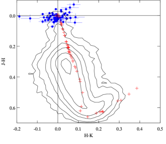
Figure 14: The $J-H$ vs $H-K$ diagram for stellar sources in the UKIDSS LAS with counterparts in SDSS. Objects are selected to be stellar in all WFCAM filters and an overall stellar SDSS classification. Measured photometric errors are $\leq 0.05$ magnitudes in each WFCAM passband. Sources with SDSS colours close to zero ($u-g,g-r,r-i,i-z$ all in the range -0.1 to 0.1) are plotted with errors. Red crosses are synthetic photometry from Hewett et al. (2006) based on the BPGS atlas (see text for details).

We can explore this in a little more detail for each of the LAS filters in turn. We use the $u-K$ colour to extend the baseline on the x-axis, and plot all WFCAM colour combinations in Fig. 15 for the $Y$$J$$H$$K$ filters. Offsets are measured from straight line fits to the blue stars. The slopes of the fits are very shallow, and thus any systematic error in the $u^{\prime}$- or $K$-band photometry will not significantly affect the measured offset. At $u-K=0.0$, we find $\Delta_{YJ}=-0.075\pm 0.007$, $\Delta_{YH}=-0.075\pm 0.018$, $\Delta_{YK}=-0.117\pm 0.018$, $\Delta_{JH}=-0.009\pm 0.012$, $\Delta_{JH}=-0.009\pm 0.012$, $\Delta_{HK}=-0.022\pm 0.024$, indicating an appreciable offset for the $Y$-band, and little or no offset in the $J$$H$$K$ filters.

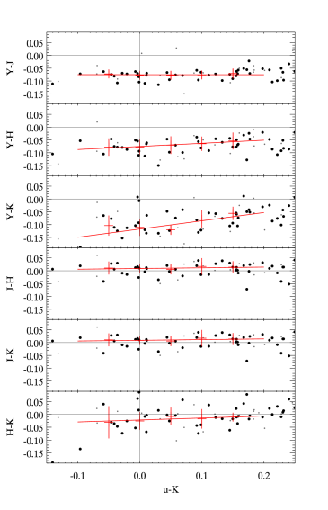
Figure 15: WFCAM colours for stellar sources in common with SDSS. Large symbols are selected to be blue in SDSS ($u-g,g-r,r-i,i-z$ all in the range -0.1 to 0.1). Error bars are the standard deviations on binned median values. The best fit straight lines are also drawn.

6.2 The $Y$-band

At the start of WFCAM observations, there was no reliable calibration for $Y$, and as a consequence an estimate of the zeropoint was made for the early data releases. To examine the $Y$-band calibration in more detail, we plot the $Y-J$ vs $J-K$ diagram in Fig. 16. The blue star sequence does not pass through (0,0), but is significantly shifted to the blue in $Y-J$. We attribute the displacement to the offset in the $Y$-band calibration in DR2. A maximum likelihood straight-line fit to the blue stars (including photometric errors, see Appendix) yields the intercept in $Y-J$, $\Delta_{Y}=-0.074\pm 0.005$.

Relaxing the source selection such that there is no requirement for a counterpart in SDSS yields a slightly larger sample. From the LAS dataset alone we measure $\Delta_{Y}=-0.080\pm 0.005$.

Fig. 16 shows that there is a non-linearity in the transformation between the $J-K$ and $Y-J$ colours for blue stars. Hence the $Y$-band offset is a natural consequence of adopting a linear extrapolation based on redder stars.

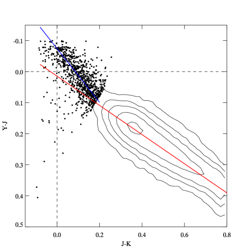
Figure 16: The DR2 $Y-J$ vs $J-K$ diagram for stellar sources common to the UKIDSS LAS and SDSS surveys. Objects are selected to be stellar in all WFCAM filters with a measured photometric error $\leq 0.05$ magnitudes in each passband. SDSS sources are selected to have a stellar classifcation and a photometric error $\leq 0.1$ in all filters. Sources in regions of significant reddening, $E(B-V)^{\prime}>0.2$ are excluded from the plot and from analysis. So-called ‘blue stars’ are plotted with a larger symbol. The best-fit straight line is shown in blue. An additional linear fit to the remaining stars is shown in red extending down to $J-K=0.8$.

6.3 The $Z$-band

The only UKIDSS survey with significant $Z$-band coverage is the Galactic Clusters Survey (GCS), with essentially no overlap with SDSS at present. In Fig. 17 we plot $Y-J$ and $Z-J$ against $J-K$, for stellar sources detected in the GCS to: (i) confirm the $Y$-band offset discussed above, (ii) check the validity of using the GCS dataset to measure the offset, and (iii) investigate a possible offset in the $Z$-band.

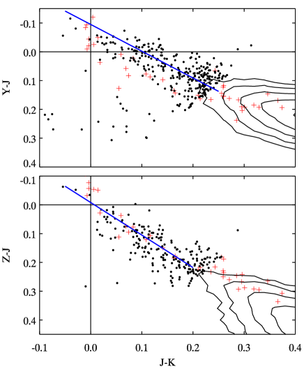
Figure 17: Colour-colour diagrams for UKIDSS GCS photometry of point sources. Red crosses are synthetic photometry from Hewett et al. (2006).

The sample of blue stars is rather smaller than derived from the LAS sample, but the offset for the $Y$-band is reproduced with $\Delta_{YJ}=-0.095\pm 0.015$. For the $Z$-band we measure an intercept of $\Delta_{ZJ}=-0.008\pm 0.015$, i.e. consistent with zero.

6.4 Summary of offsets

In summary, an offset to the WFCAM $Y$-band zeropoint needs to be applied to bring it onto the Vega photometric system. We take the weighted mean of the various values derived above with respect to the WFCAM $J$-band and the SDSS $i$-band, and find $\Delta_{Y}=-0.078\pm 0.010$. Consequently an offset of 0.080 has been applied for UKIDSS DR3 and subsequently as shown in Equation 5.

For the $ZJHK$-bands, the data are consistent with no offset at the $\pm 2$ per cent level.

7 Comparison with published $J$$H$$K$ photometry in the Mauna Kea Observatories photometric system

Every night that WFCAM is observing, a number of standard fields are measured, typically every two hours (in the first year of operations this was an hourly procedure). The majority of the standard fields include stars selected from the list of UKIRT faint standards published in Hawarden et al. (2001). These fields were initially chosen to act as the primary source of photometric calibration for WFCAM, however, subsequent analysis (presented in this paper) has demonstrated that the 2MASS-based calibration offers significant advantages. Observations of standard stars currently continue to be performed at the telescope, to ensure that a future calibration can be derived independently from 2MASS should the need arise. The standard observations also enable monitoring of the WFCAM system by the reliable strategy of repeatedly looking at the same stars.

Recently, Leggett et al. (2006) have revisited the UKIRT faint standards, and present new measurements using the UKIRT Fast Track Imager (UFTI). They find small offsets (at the few per cent level) with respect to the older data, as well as some evidence of magnitude-dependent non-linearity, and recommend adopting the newer photometry.

In Fig. 18 we compare the DR3 WFCAM calibration with the recalibrated UFTI photometry of faint standard stars measured in the Mauna Kea Observatories system (Leggett et al. 2006).

Figure 18: Median $\Delta$mag (WFCAM minus UFTI photometry) plotted as a function of $J-K$ (UFTI) for the $J$, $H$ and $K$ filters (top to bottom). The dashed lines show the median measured offsets between the WFCAM and UFTI photometry, discussed in the text.

WFCAM measurements were selected from observations taken on photometric nights during good conditions. There are typically 50–100 measurements per star in each filter. The data values plotted are the median $\rm m_{\rm w}-m_{UFTI}$ for the $J$$H$$K$ filters, and error bars are the standard deviation calculated as 1.48$\times$ the median absolute deviation (MAD) of the WFCAM measurements. Only stars passing the following criteria are plotted and analysed: (i) they show no variability ($rms_{JHK}<=0.03$); (ii) they are fainter than $J$$H$$K$=11 to avoid possible saturation/non-linearity effects. Thus the sample is rather small, and does not include any objects with extreme colours.

Most stars are not variable at the 1–2 per cent level, but we note a few exceptions: FS117 (b216-b9), FS143 (Ser-EC86), GSPC P259-C, which all show evidence for variability at $\geq 5$ per cent within the timeframe of the observations (2005 April–2007 May). As in Leggett et al. (2006), we find FS144 (Ser-EC84) may be variable at the 3 per cent level. However, we find no evidence to suggest that FS116 (b216-b7) is variable at $\geq 1$ per cent.

Over the limited colour range considered in Fig. 18, we do not see evidence for a colour term between the $J_{\rm w}$ and $J_{\rm UFTI}$ photometry. However, a larger sample of stars with both UFTI and WFCAM photometry, spanning a broader colour range, is required before a definitive statement can be made. The median measured offsets between the WFCAM and UFTI photometry are: $\delta_{J}=0.005$, $\delta_{H}=0.015$, $\delta_{K}=0.017$. WFCAM-UFTI is positive in the three filters, i.e. the WFCAM measurements are slightly fainter. Leggett et al. (2006) also measured small offsets between the WFCAM and UFTI systems; and find a different offset in the $H$-band, with $H_{\rm w}-H_{\rm UFTI}\sim-0.015$. We note that the Leggett et al. (2006) measurements are based on an earlier WFCAM calibration, and use a sample of stars without such a restrictive magnitude cut and comprising many fewer repeat observations.

During the WFCAM Science Verification phase (2005 April), a decision was taken to anchor the WFCAM calibration to the Hawarden et al. (2001) UKIRT photometry. An offset of 0.03 magnitudes was found between the 2MASS-based WFCAM calibration and the UKIRT system, thus requiring a correction to the colour equation (Equation 7) for the $H$-band. When making this decision, we were also aware that Cohen et al. (2003) argued for small offsets to be applied to the 2MASS $H_{2}$ and $K_{2}$ bands to bring them into agreement with their space-based infrared spectrophotometric calibration system (the offset required for $J_{2}$ is negligible). The suggested offsets, to be applied to the published 2MASS photometry, were $-0.019\pm 0.007$ ($H_{2}$), and $+0.017\pm 0.005$ ($K_{2}$).

At present, in the absence of a larger sample of observations and more-accurate photometry, we conclude that the WFCAM photometric system is a Vega system (to within 2 per cent) and is in agreement with all three of the Hawarden et al. (2001), Cohen et al. (2003) and Leggett et al. (2006) systems to within 2 per cent. For the time being we choose to retain the 3 per cent offset in the conversion between the 2MASS and WFCAM $H$-band photometry.

8 Empirical determination of the throughput of WFCAM

8.1 Gain

Measurements of the readout noise and gain from the 2005 April SV data are given in Table 5. The readout noise was estimated from the difference between successive single exposure CDS 5 s dark frames after running the decurtaining algorithm to remove systematic artifacts. Note that the average dark current is generally negligible and dominated by reset anomaly variations. The gain is the average of gains measured at three background levels 23k, 14k and 5k; the overall variation in measured gain was at the  0.05 level with no clear trends with background.

Table 5: Measured dark current, uncorrected gain and noise (in electrons and ADU) for the four WFCAM detectors. The gain is an overestimate, as described in the text. The corrected average gain for WFCAM is 4.31.

Det	Dark curr.	Noise (ADU)	Uncorr. gain	Noise (e-)
#1	-2.4	3.8	4.84	18.4
#2	3.7	4.2	4.87	20.5
#3	-9.0	4.2	5.80	24.4
#4	49.1	4.4	5.17	22.7

Whilst measuring the gain from the dome flat sequences, an estimate of the inter-pixel capacitance via a robust measure of the noise covariance matrix was also made. A sum of the noise covariance matrix close to 0,0 gives a value of 1.20 which implies that the total reduction in directly measured noise variance (i.e. measured using a conventional method) is therefore also 1.20. We therefore predict a  20 per cent overestimate of the gain, and hence a  20 per cent overestimate of the QE coefficients. Such an overestimate is as expected for the Rockwell Hawaii-II devices. The average gain of the WFCAM detectors is therefore 4.31.

8.2 Throughput

The total throughput of the system is relatively easy to measure (but it is much harder to quantify where in the system the actual losses are occurring). For the calculation we have assumed the following: The effective area of the UKIRT primary mirror is 10.5m² (i.e. outer diameter 3.802m with an inner diameter of 1.028m). No attempt has been made to allow for the shadowing of the primary by the secondary, nor for any obscuration caused by the forward mounted camera itself. The spectrum for Vega is the same used by Hewett et al. (2006), originally from Bohlin & Gilliland (2004). The passband transmissions are from Hewett et al. (2006) but renormalized to give the relative throughput as a function of wavelength, rather than absolute transmission (i.e. the peak value is 1.0).

Thus Table 7 gives the estimated number of photons that would be incident on the primary mirror, assuming no atmosphere, multiplied by the relative transmission of the filter in each band. The values in table 7 allow the calculation of the zeropoint of the system in each filter assuming no losses due to the atmosphere, telescope and the instrument. Comparison with the median measured zeropoints for DR1 then give us the throughput for WFCAM+UKIRT+atmosphere.

Table 6: Estimate of WFCAM throughput

Filt	Nν(0m)	NC(0m)	ZP100	ZP (M)	TPM
$Z_{\rm w}$	3.7e10	8.5e9	24.95	22.77	15%
$Y_{\rm w}$	3.1e10	7.3e9	24.77	22.78	18%
$J_{\rm w}$	2.9e10	6.8e9	24.70	22.97	23%
$H_{\rm w}$	2.8e10	6.6e9	24.66	23.22	29%
$K_{\rm w}$	1.6e10	3.6e9	24.02	22.55	29%

Table 7: Where N_ν is the number of photons reaching the detector in each passband for a zeroth magnitude star, N_c is the equivalent number of counts in the detector and ZP₁₀₀ is the corresponding predicted zeropoint for each filter if there were no losses in the system. ZP_M is the actual measured median zeropoint for WFCAM in each filter, and TP_M is therefore the adjusted throughput of the system compared to a perfect instrument and atmosphere.

9 Conclusions

1. The CASU pipeline photometric calibration of WFCAM data, using 2MASS sources within each WFCAM pointing, has achieved a photometric accuracy better than 2 per cent for the UKIDSS Large Area Survey released in DR3 (Data Release 3) and later, based on repeat measurements.

2. By stacking spatially binned WFCAM data on monthly timescales we have shown that photometric calibration residuals are present at the 1 per cent level. We have derived and tested a method for removing these residuals, and show that the photometric calibration for the WFCAM $J$$H$$K$ filters can reach an accuracy of 1.5 per cent. We attribute these residuals to scattered light in the WFCAM twilight flatfield frames. These corrections have been applied to the UKIDSS DR4.

3. Even observations taken through thin cloud (where transmission is $>$ 80 per cent) can be calibrated to $\sim$ 2 per cent using 2MASS calibrators.

4. Monte-Carlo sampling the 2MASS stars observed by WFCAM, suggests that as long as $\sim$ 50 calibrators fall within the field-of-view, then the WFCAM calibration is robust to 1 per cent in $Y$$J$$H$$K$ and 2 per cent in $Z$. 99 per cent of the sky has more than 50 2MASS calibrators in a single WFCAM pointing.

5. The WFCAM calibration incorporates colour restrictions on secondary standards and modified colour equations to mitigate against the effects of Galactic extinction. Towards regions of significant reddening, the calibration meets the 2 per cent requirement for $E(B-V)^{\prime}\leq 2.0$ for the $J$$H$$K$ bands, but should be treated with caution above $E(B-V)^{\prime}=0.2$ for the $Z$ band and to a lesser extent for the $Y$ band.

6. We find that the calibration of WFCAM from the shallower 2MASS survey is free from the effects of Eddington Bias, thanks to a careful choice of a signal-to-noise cut (SNR$=10$) for the 2MASS sources.

7. We identified a small offset between the WFCAM $Y$ photometry and an idealized Vega photometric system in the second UKIDSS Data Release (DR2). A correction of $\Delta_{Y}=-0.08$ magnitudes has now been included in the WFCAM calibration and applied from UKIDSS DR3, in the sense that the $Y$ band sources are now 0.08 magnitues fainter than in previous releases.

8. We find that the WFCAM photometric system is within 0.02 magnitudes of the UKIRT MKO system (Leggett et al. 2006) for the $J$$H$$K$ filters, and is Vega-like to within 2 per cent (i.e. stars selected to have A0 colours in SDSS have WFCAM colours $<=0.02$ across all passbands).

Appendix A Structural Analysis

We use the blue end of the distribution of points culled from the GCS to illustrate the problem of finding an accurate estimate for the $Y$-band offset. In this case, since the WFCAM $J$,$K$-bands are already on the Vega system, this is equivalent to finding the intercept on the $Y-J$ axis when the $J-K$ colour is zero. However, with significant errors on both axes, and possibly also an intrinsic spread in the stellar locus, conventional least-squares curve fitting methods can give seriously biased results. This is illustrated in Fig. 19 where the obvious outliers (red points) have been excluded from the fits. In this example we have (arbitrarily) defined the x-axis to be the $J-K$ measures and the y-axis to be the $Y-J$ measures. The green dashed line shows the result of a standard variance-weighted least-squares regression of $y$ on $x$, while the blue dashed line shows the same for a regression of $x$ on $y$. The values of the supposedly equivalent slopes and intercepts are significantly different and the clear bias in both fits is simply the result of ignoring the duality of the error distribution. We note that an often-used shortcut for this type of situation is simply to “average” the results from the two regressions and use that for the solution. As it happens, if the magnitude of the errors on both axes are similar this often gives a result close to the optimum value.

The correct procedure in this type of case is to explicitly recognise the more complex error distribution involved by rephrasing the modelling problem in terms of the unobserved “true” parameters using the method of maximum likelihood. This technique is also known as structural analysis (e.g. Kendall & Stuart 1979).

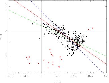
Figure 19: Locating the offset in the $Y$-band calibration for WFCAM using standard least-squares regression (green and blue lines) compared to the correct Maximum likelihood technique (red line). Red filled points are excluded from all the fits.

In general terms the underlying model is of the form $Y_{i}=f(X_{i}\mid\theta)$, whereas what we observe are not these values but rather the quantities $x_{i}=X_{i}+\delta x_{i}$ and $y_{i}=Y_{i}\ +\delta y_{i}$ where $\delta x_{i}$ and $\delta y_{i}$ are independent errors with variance $\sigma^{2}_{x_{i}}$ ,  $\sigma^{2}_{y_{i}}$ which may include intrinsic spread in the model as well as observational and calibration errors. If these errors are Gaussian distributed then the likelihood $L$ of observing the $N$ independent pairs of values $x_{i},y_{i}$ is given by

$$L=\prod_{i=1}^{N}\ P(x_{i},y_{i}\mid\theta)$$ (14)

where $\theta$ represent the model parameters; and the log-likelihood is therefore given by

$$ln(L)=-N\ ln(2\pi)-{1\over 2}\ \sum_{i}\ ln(\sigma^{2}_{x_{i}}.\sigma^{2}_{y_{i}})-{1\over 2}\sum_{i}\left({\delta x_{i}^{2}\over\sigma^{2}_{x_{i}}}+{\delta y_{i}^{2}\over\sigma^{2}_{y_{i}}}\right)$$ (15)

For unknown errors the problem is insoluble. For known errors

$$ln(L)=const-{1\over 2}\sum_{i}{[x_{i}-X_{i}]^{2}\over\sigma^{2}_{x_{i}}}+{[y_{i}-Y_{i}]^{2}\over\sigma^{2}_{y_{i}}}$$ (16)

and the solution effectively involves solving for $X_{i}$ and $\theta_{j}$ i.e. $N+m$ unknowns, often using a mixture of a direct parameter search on $ln(L)$ in conjunction with the following differential constraints

$${\partial ln(L)\over\partial X_{i}}={(x_{i}-X_{i})\over\sigma^{2}_{x_{i}}}+{\partial f\over\partial X_{i}}\ \left[{y_{i}-f(X_{i}\mid\theta)\over\sigma^{2}_{y_{i}}}\right]=0$$ (17)

$${\partial ln(L)\over\partial\theta_{j}}=\sum_{i}\ {\partial f\over\partial\theta_{j}}\ \left[{y_{i}-f(X_{i}\mid\theta)\over\sigma^{2}_{y_{i}}}\right]=0$$ (18)

Figure 20: Log-likelihood contours starting at 1-$\sigma$ and spaced by intervals of 1-$\sigma$ for the maximum likelihood model fit shown for the data presented in figure 19

We illustrate the use of this technique to find the intercept using the straight line model defined by $Y_{i}=aX_{i}+b$. In this case the differential constraint on $X_{i}$ (equation 17) simplifies to

$${x_{i}-X_{i}\over\sigma^{2}_{x_{i}}}+{a(y_{i}-aX_{i}-b)\over\sigma^{2}_{y_{i}}}=0$$ (19)

which implies for a given parameter pair $(a,b)$ that $X_{i}$ is determined by

$$X_{i}={ay_{i}-ab+x_{i}\lambda_{i}^{2}\over a^{2}+\lambda_{i}^{2}}$$ (20)

where we have defined $\lambda_{i}^{2}={\sigma^{2}_{y_{i}}\over\sigma^{2}_{x_{i}}}$.

Given $X_{i}$ and a trial pair $(a,b)$, $Y_{i}$ is defined by the model and it is then straightforward to compute the log-likehood function using a direct search on a suitable grid of values $(a,b)$. The result of doing this for the data presented in Fig. 19 is shown in the log-likelihood contours in Fig. 20.

Appendix B SQL

An example WFCAM Science Archive SQL query for the selection of repeat $K$-band observations in the Large Area Survey. Note that the s1.sourceID < s2.sourceID qualifier is used to ensure that each match appears only once in the output results (and not twice as would happen otherwise).

SELECT s1.kAperMag3 as mag1,s2.kAperMag3 as mag2

FROM   lasSource s1,lasSource s2,
       lasMergeLog l1,lasMergeLog l2,
       lasDetection d1,lasDetection d2,
       MultiframeDetector f1,MultiframeDetector f2,
       CurrentAstrometry c1,CurrentAstrometry c2
       lasSourceNeighbours x,

WHERE  s1.sourceID = x.masterObjID AND
       s2.sourceID = x.slaveObjID AND
       s1.frameSetID = l1.frameSetID AND
       s2.frameSetID = l2.frameSetID AND
       s1.kAperMag3Err < 0.12 AND
       s2.kAperMag3Err < 0.12 AND
       s1.kclass = -1 AND
       s2.kclass = -1 AND
       f1.multiframeID = c1.multiframeID AND
       f2.multiframeID = c2.multiframeID AND
       f1.extNum = c1.extNum AND
       f2.extNum = c2.extNum AND
       d1.multiframeID = f1.multiframeID AND
       d2.multiframeID = f2.multiframeID AND
       d1.extNum = f1.extNum AND
       d2.extNum = f2.extNum AND
       d1.objID = s1.kObjID AND
       d2.objID = s2.kObjID AND
       l1.kmfID = f1.multiframeID AND
       l2.kmfID = f2.multiframeID AND
       l1.keNum = f1.extNum AND
       l2.keNum = f2.extNum AND
       s1.frameSetID <> s2.frameSetID AND
       s1.sourceID < s2.sourceID AND
       distanceMins < (0.3/60.0) AND
       distanceMins IN (
              SELECT  MIN(distanceMins)
              FROM    lasSourceNeighbours
              WHERE   masterObjID=x.masterObjID
                       )

Appendix C Conversion of flux into magnitudes

The processing philosophy is to preserve the image and catalogue data as counts, and to document all the required calibration information in the file headers. Thus recalibration of the data requires only changes to the headers, and these headers can be reingested into the WSA without the need to reingest the full tables. For readers accessing the flat files (catalogues and images) rather than the WSA database products, we document the methods for converting the fluxes into magnitudes and calibrating the photometry.

$$m=ZP-2.5log_{\rm 10}(\frac{f}{t})-A-2.5log_{\rm 10}(\frac{f_{\rm cor}}{f})-k(\chi-1)$$ (21)

where $ZP$ is the zeropoint for the frame (keyword: MAGZPT in the FITS header), $f$ is the flux within the chosen aperture (e.g. column: APER_FLUX_5), $t$ is the exposure time for each combined integration (keyword: EXP_TIME), and $A$ is the appropriate aperture correction (e.g. keyword: APCOR5). The next term deals with the distortion correction caused by the varying pixel scale, where ($f_{\rm cor}/f$) is the correction and is derived in Equation 1. The final term deals with the extinction correction, where $k$ is the extinction coefficient (EXTINCTION) and is equal to 0.05 magnitudes/airmass in all filters, and $\chi$ is the airmass (keywords: AMSTART, AMEND).

Appendix D Relevant source and image parameters

Table 8: Table of source parameters generated by the WFCAM pipeline and written to the FITS catalogue products, and an accompanying short description for each.

1	Sequence number	Running number for ease of reference, in strict order of image detections.
2	Isophotal flux	Standard definition of summed flux within detection isophote, apart from detection filter is used to define pixel connectivity and hence which pixels to include. This helps to reduce edge effects for all isophotally derived parameters.
3	X coord	Intensity-weighted isophotal centre-of-gravity in X.
4	Error in X	Estimate of centroid error.
5	Y coord	Intensity-weighted isophotal centre-of-gravity in Y.
6	Error in Y	Estimate of centroid error.
7	Gaussian sigma	Derived from the three intensity-weighted second moments. The equivalence to a generalised elliptical Gaussian distribution is used to derive: Gaussian sigma = $(\sigma_{a}^{2}+\sigma_{b}^{2})^{1/2}$
8	Ellipticity	ellipticity = $1.0-\sigma_{a}/\sigma_{b}$
9	Position angle	position angle = angle of ellipse major axis wrt x axis
10–16	Areal profile 1 Areal profile 2 Areal profile 3 Areal profile 4 Areal profile 5 Areal profile 6 Areal profile 7	Number of pixels above a series of threshold levels relative to local sky. Levels are set at T, 2T, 4T, 8T … 128T where T is the threshold. These can be thought of as a poor man’s radial profile. For deblended, i.e. overlapping images, only the first areal profile is computed and the rest are set to -1.
17	Areal profile 8	For blended images this parameter is used to flag the start of the sequence of the deblended components by setting the first in the sequence to 0
18	Peak height	In counts relative to local value of sky - also zeroth order aperture flux
19	Error in peak height
20–45	Aperture flux 1 Error in flux Aperture flux 2 Error in flux Aperture flux 3 Error in flux Aperture flux 4 Error in flux Aperture flux 5 Error in flux Aperture flux 6 Error in flux Aperture flux 7 Error in flux Aperture flux 8 Error in flux Aperture flux 9 Error in flux Aperture flux 10 Error in flux Aperture flux 11 Error in flux Aperture flux 12 Error in flux Aperture flux 13 Error in flux	These are a series of different radius soft-edged apertures designed to adequately sample the curve-of-growth of the majority of images and to provide fixed-sized aperture fluxes for all images. The scale size for these apertures is selected by defining a scale radius $\sim<$FWHM$>$ for site+instrument. In the case of WFCAM this ”core” radius (rcore) has been fixed at 1.0 arcsec for convenience in inter-comparison with other datasets. A 1.0 arcsec radius is equivalent to 2.5 pixels for non-interleaved data, 5.0 pixels for 2x2 interleaved data, and 7.5 pixels for 3x3 interleaved data. In $\sim$1 arcsec seeing an rcore-radius aperture contains roughly 2/3 of the total flux of stellar images. (The rcore parameter is user specifiable and hence is recorded in the output catalogue FITS header.) The aperture fluxes are sky-corrected integrals (summations) with a soft-edge (i.e. pro-rata flux division for boundary pixels). However, for overlapping images the fluxes are derived via simultaneously fitted top-hat functions, to minimise the effects of crowding. Images external to the blend are also flagged and not included in the large radius summations. Aperture flux 3 is recommended if a single number is required to represent the flux for ALL images - this aperture has a radius of rcore. Starting with parameter 20 the radii are: (1) $1/2\times$rcore, (2) $1/\sqrt{2}\times$rcore, (3) rcore, (4) $\sqrt{2}\times$rcore, (5) $2\times$rcore, (6) $2\sqrt{2}\times$rcore, (7) $4\times$rcore, (8) $5\times$rcore, (9) $6\times$rcore, (10) $7\times$rcore, (11) $8\times$rcore, (12) $10\times$rcore, (13) $12\times$rcore. Note $4\times$rcore contains $\sim$99% of PSF flux. The apertures beyond Aperture 7 are for generalised galaxy photometry. Note larger apertures are all corrected for pixels from overlapping neighbouring images. The largest aperture has a radius 12$\times$rcore ie. $\sim$24 arcsec diameter. The aperture fluxes can be combined with later-derived aperture corrections for general purpose photometry and together with parameter 18 (the peak flux) give a simple curve-of-growth measurement which forms the basis of the morphological classification scheme.
46	Petrosian radius	$r_{p}$ as defined in Yasuda et al. 2001 AJ 112 1104
47	Kron radius	$r_{k}$ as defined in Bertin and Arnouts 1996 A&A Supp 117 393
48	Hall radius	$r_{h}$ image scale radius eg. Hall & Mackay 1984 MNRAS 210 979

49	Petrosian flux	Flux within circular aperture to $k\times r_{p}$; $k$ = 2
50	Error in flux
51	Kron flux	Flux within circular aperture to $k\times r_{k}$; $k$ = 2
52	Error in flux
53	Hall flux	Flux within circular aperture to $k\times r_{h}$; $k$ = 5; alternative total flux
54	Error in flux
55	Error bit flag	Bit pattern listing various processing error flags
56	Sky level	Local interpolated sky level from background tracker
57	Sky $rms$	local estimate of $rms$ in sky level around image
58	Child/parent	Flag for parent or part of deblended deconstruct (redundant since only deblended images are kept)
59-60	RA DEC	RA and Dec explicitly put in columns for overlay programs that cannot, in general, understand astrometric solution coefficients - note r*4 storage precision accurate only to ∼50mas. Astrometry can be derived more precisely from WCS in header and XY in parameters 5 & 6
61	Classification	Flag indicating most probable morphological classification: eg. -1 stellar, +1 non-stellar, 0 noise, -2 borderline stellar, -9 saturated
62	Statistic	An equivalent N(0,1) measure of how stellar-like an image is, used in deriving parameter 61 in a ”necessary but not sufficient” sense. Derived mainly from the curve-of-growth of flux using the well-defined stellar locus as a function of magnitude as a benchmark (see Irwin et al. 1994 SPIE 5493 411 for more details).

Table 9: Relevant photometric parameters measured by the pipeline and written to the FITS headers. These values are computed per-detector and stored in the headers for each image and catalogue extension. The names by which the parameters are stored in the WFCAM Science Archive tables are also given.

FITS keyword	WSA parameter	Description
AMSTART	amStart	Airmass at start of observation
AMEND	amEnd	Airmass at end of observation
PIXLSIZE	pixelScale	$[$arcsec$]$ Pixel size
SKYLEVEL	skyLevel	$[$counts/pixel$]$ Median sky brightness
SKYNOISE	skyNoise	$[$counts$]$ Pixel noise at sky level
THRESHOL	thresholdIsoph	$[$counts$]$ Isophotal analysis threshold
RCORE	coreRadius	$[$pixels$]$ Core radius for default profile fit
SEEING	seeing	$[$pixels$]$Average stellar source FWHM
ELLIPTIC	avStellarEll	Average stellar ellipticity (1-b/a)
APCORPK	aperCorPeak	$[$magnitudes$]$ Stellar aperture correction – peak height
APCOR1	aperCor1	$[$magnitudes$]$ Stellar aperture correction – core/2 flux
APCOR2	aperCor2	$[$magnitudes$]$ Stellar aperture correction – core/$\sqrt{2}$ flux
APCOR3	aperCor3	$[$magnitudes$]$ Stellar aperture correction – core flux
APCOR4	aperCor4	$[$magnitudes$]$ Stellar aperture correction – $\sqrt{2}\times$ core flux
APCOR5	aperCor5	$[$magnitudes$]$ Stellar aperture correction – $2\times$ core flux
APCOR6	aperCor6	$[$magnitudes$]$ Stellar aperture correction – $2\sqrt{2}\times$ core flux
APCOR7	aperCor7	$[$magnitudes$]$ Stellar aperture correction – $4\times$ core flux
MAGZPT	photZPExt	$[$magnitudes$]$ Photometric ZP for default extinction
MAGZRR	photZPErrExt	$[$magnitudes$]$ Photometric ZP error
EXTINCT	extinctionExt	$[$magnitudes$]$ Extinction coefficient
NUMZPT	numZPCat	Number of 2MASS standards used
NIGHTZPT	nightZPCat	$[$magnitudes$]$ Average photometric ZP for the filter for the night
NIGHTZRR	nightZPErrCat	$[$magnitudes$]$ Photometric ZP $\sigma$ for the filter for the night
NIGHTNUM	nightZPNum	Number of ZPs measured for the filter for the night

References

- Bohlin & Gilliland (2004) Bohlin R. C., Gilliland R. L., 2004, AJ, 127, 3508
- Bonifacio, Monai & Beers (2000) Bonifacio P., Monai S., Beers T. C., 2000, AJ, 120, 2065
- Casali et al. (2007) Casali M. et al., 2007, A&A, 467, 777
- Cohen, Wheaton, & Megeath (2003) Cohen M., Wheaton W. A., Megeath S. T., 2003, AJ, 126, 1090
- Cruz et al. (2003) Cruz K., L., Reid I. N., Liebert J., Kirkpatrick J. D., Lowrance P. J., 2003, AJ, 126, 2412
- Cutri et al. (2003) Cutri R. M., Skrutskie M. F., Van Dyk S., et al., 2003, Explanatory Supplement to the 2MASS All Sky Data Release, IPAC
- Eddington (1940) Eddington A. S., 1940, MNRAS, 100, 354
- Hambly et al. (2008) Hambly N. C., Collins R. S., Cross N. J. G., Mann R. G., Read M. A., Sutorius E. T. W., Bond I., Bryant J., Emerson J. P., Lawrence A., Rimoldiniw L., Stewart J. M., Williams P. M., Adamson A., Hirst P., Dye S., Warren S. J., 2008, MNRAS, 384, 637
- Hawarden et al. (2001) Hawarden T. G., Leggett S. K., Letawsky M. B., Ballantyne D. R., Casali M. M., 2001, MNRAS, 325, 563
- Hewett et al. (2006) Hewett P. A, Warren S. J., Leggett, S. K., Hodgkin S. T., 2006, MNRAS, 367, 454
- Irwin et al. (2008) Irwin M., Leiws J., Riello M., Hodgkin S. T., Gonzales-Solares E., Evans D. W., Bunclark P.S., 2008, in prep
- Irwin (1985) Irwin M., 1985, MNRAS, 214, 575
- Lawrence et al. (2007) Lawrence A. J. et al., 2007, MNRAS, 379, 1599
- Leggett et al. (2000a) Leggett S. K., Allard F., Dahn C., Hauschildt P. H., Kerr T. H., Rayner J., 2000a, ApJ, 535, 965
- Leggett et al. (2000b) Leggett S. K., et al., 2000b, ApJ, 536, L35
- Leggett et al. (2001) Leggett S. K., Allard F., Geballe T. R., Hauschildt P. H., Schweitzer A., 2001, ApJ, 548, 908
- Leggett et al. (2002a) Leggett S. K., Hauschildt P. H., Allard F., Geballe T. R., Baron E., 2002a, MNRAS, 332, 78
- Leggett et al. (2002b) Leggett S. K., et al., 2002b, ApJ, 564, 452
- Leggett et al. (2006) Leggett S. K., Currie M. J., Varricatt W. P., Hawarden T. G., Adamson A. J., Buckle J., Carroll T., Davies J. K., Davis C. J., Kerr T. H., Kuhn O. P., Seigar M. S., Wold T., 2006, MNRAS, 373, 781
- Nikolaev et al. (2000) Nikolaev S., Weinberg M. D., Skrutskie M. F., Cutri R. M., Wheelock S. L., Gizis J. E., Howard E. M., 2000, AJ, 120, 3340
- Schlegel et al. (1998) Schlegel D. J., Finkbeiner D. P., & Davis M., 1998, ApJ, 500, 525
- Skrutskie et al. (2006) Skrutskie et al., 2006, AJ, 131, 1163
- Tokunaga, Simons, & Vacca (2002) Tokunaga A. T., Simons D. A., Vacca W. D., 2002, PASP, 114, 180
- Tokunaga & Vacca (2005) Tokunaga A. T., Vacca W. D., 2005, PASP, 117, 421
- Warren et al. (2007) Warren S. J. et al. 2007, MNRAS, 375, 213
- Warren & Hewett (2002) Warren S. J., Hewett P., 2002, ASPC, 283, 369