HeII$\rightarrow$HeI Recombination of Primordial Helium Plasma Including the Effect of Neutral Hydrogen

E. E. Kholupenko¹, A. V. Ivanchik^1,2, and D. A. Varshalovich^1,2

¹Ioffe Physical-Technical Institute of RAS, Russia
²St. Petersburg State Polytechnical University, Russia

Abstract

The HeII$\rightarrow$HeI recombination of primordial helium plasma ($z=1500-3000$) is considered in terms of the standard cosmological model. This process affects the formation of cosmic microwave background anisotropy and spectral distortions. We investigate the effect of neutral hydrogen on the HeII$\rightarrow$HeI recombination kinetics with partial and complete redistributions of radiation in frequency in the HeI resonance lines. It is shown that to properly compute the HeII$\rightarrow$HeI recombination kinetics, one should take into account not only the wings in the absorption and emission profiles of the HeI resonance lines, but also the mechanism of the redistribution of resonance photons in frequency. Thus, for example, the relative difference in the numbers of free electrons for the model using Doppler absorption and emission profiles and the model using a partial redistribution in frequency is 1 - 1.3% for the epoch $z=1770-1920$. The relative difference in the numbers of free electrons for the model using a partial redistribution in frequency and the model using a complete redistribution in frequency is 1 - 3.8% for the epoch $z=1750-2350$.

PACS numbers : 98.80.-k
DOI: 10.1134/S1063773708110017

Key words: cosmology, primordial plasma, recombination, cosmic microwave background, anisotropy, radiation transfer, continuum absorption, continuum opacity, escape probability

1 Introduction

The recombination of primordial plasma is a process that ultimately leads to the formation of neutral atoms from ions and free electrons due to the decrease in temperature through cosmological expansion. This process has three distinct epochs at which the fraction of free electrons changes significantly: (1) HeIII$\rightarrow$HeII recombination ($z\simeq 5000-7000$), (2) HeII$\rightarrow$HeI recombination ($z\simeq 1500-3000$), and (3) HII$\rightarrow$HI recombination ($z\simeq 900-1600$), where z is the cosmological redshift. Since other nuclides (D, ³He, Li, B, etc.) in the primordial plasma are much fewer in number than ¹H and ⁴He ($<10^{-4}$), the recombination of hydrogen-helium plasma is usually considered (Zeldovich et al. 1968; Peebles 1968; Matsuda et al. 1969). The recombination of other elements is considered in isolated cases for special problems, such as the effect of lithium recombination on the cosmic microwave background (CMB) anisotropy (Stancil et al. (2002) and references therein), the formation of primordial molecules (Galli and Palla (2002) and references therein), etc.

The recombination of primordial plasma affects significantly the growth of gravitational instability and the formation of CMB spectral distortions and anisotropy (Peebles 1965; Dubrovich 1975). The appearance of the first experimental data on CMB anisotropy (Relikt 1, COBE) rekindled interest in the recombination of primordial plasma in the mid- 1980s. A number of improvements in the model of hydrogen plasma recombination were suggested (Jones and Wyse 1985; Grachev and Dubrovich 1991).

Significant progress in CMB anisotropy observations achieved in the second half of the 1990s (BOOMERANG, WMAP) necessitated including a number of subtle effects that could affect the recombination of primordial hydrogen and helium at a level of 0.1 - 1% (Leung et al. 2004; Dubrovich and Grachev 2005; Novosyadlyj 2006; Burgin et al. 2006; Kholupenko and Ivanchik 2006; Wong and Scott 2007; Chluba and Sunyaev 2006, 2007, 2008a, 2008b; Hirata and Switzer 2008; Sunyaev and Chluba 2008; Hirata 2008; Grachev and Dubrovich 2008).

One of the most important (for the primordial plasma recombination kinetics) effects considered in recent years is the absorption of HeI resonance photons by neutral hydrogen, which leads to an acceleration of the HeII$\rightarrow$HeI recombination (Kholupenko et al. 2007 [hereinafter KhIV07]; Switzer and Hirata 2008; Rubino-Martin et al. 2007). Recently, this effect was taken into account by Wong et al. (2008) in the recfast computational code developed by Seager et al. (1999). This code is most widely used to compute the primordial plasma recombination kinetics when the CMB anisotropy is analyzed. To take into account the effect of neutral hydrogen on the HeII$\rightarrow$HeI recombination kinetics, Wong et al. (2008) used a simple approximation formula with adjustable parameters. The recfast modified in this way allows the results of computations with the multilevel code by Switzer and Hirata (2008) to be quickly and accurately reproduced for any reasonable values of the cosmological parameters. Nevertheless, the approach by Wong et al. (2008) is inapplicable for more detailed studies of the helium recombination, since their formula is not universal for all resonance transitions in HeI, but can be used only in describing the absorption of HeI $2^{1}P\rightarrow 1^{1}S$ resonance photons by neutral hydrogen. When using the multilevel codes by Switzer and Hirata (2008) and Rubino-Martin et al. (2007), which allow the absorption of HeI $nP\rightarrow 1S$ ($n\geq 2$) resonance photons by neutral hydrogen to be taken into account, much of the radiative transfer calculations in the HeI resonance lines are performed numerically, which is computationally demanding and time-consuming. These circumstances forced us to seek for an analytic approach to the problem of including the effect of neutral hydrogen on the HeII$\rightarrow$HeI recombination kinetics that, on the one hand, would be more universal than the approach of Wong et al. (2008) (i.e., would allow the effect of the absorption of HeI $nP\rightarrow 1S$ resonance photons (where $n\geq 2$, and not only $n=2$) on the HeII$\rightarrow$HeI recombination to be estimated) and, on the other hand, would not reduce the speed and accuracy of the primordial plasma recombination computations for various parameters of the cosmological model. This approach was implemented on the basis of the papers by Chugai (1987) and Grachev (1988), who analytically investigated the diffusion of resonance radiation in the presence of continuum absorption. In this paper, we present extended and more detailed justifications of the key suggestions made in KhIV07. We take into account the fact that the scattering in the HeI resonance lines (for transitions in the singlet structure of the HeI atom) occurs with a partial redistribution in frequency, which turns out to be important for the results (Switzer and Hirata 2008; Rubino-Martin et al. 2007). Thus, our goal is to numerically compute the HeII$\rightarrow$HeI recombination kinetics using analytic formulas (Chugai 1987; Grachev 1988; this paper) to allow for the peculiarities of the radiative transfer in the HeI resonance lines (a partial redistribution of HeI resonance photons in frequency and their absorption in the neutral hydrogen continuum).

2 Physical model of HeII$\rightarrow$HeI recombination

In the process of cosmological recombination, the plasma deviates from its ionization equilibrium. A necessary condition for this deviation is plasma opacity for the intrinsic resonance recombination radiation. This means that the emitted resonance photon is absorbed by another neutral atom almost instantly (compared to the characteristic recombination and ionization time scales). Since the recombination radiation is excessive with respect to the equilibrium background with a blackbody spectrum, the populations of excited atomic states exceed their equilibrium values. The excess of the excited-state populations entails an increase of ionization fraction compared to its equilibrium value and, accordingly, leads to a delay of recombination. In this situation, the plasma recombination can no longer be described by the Saha formula and kinetic equations should be invoked to describe the behavior of the excited-state populations of neutral atoms and the plasma ionization fraction. The total recombination rate $J_{tot}$ [cm^-3s^-1] (dependent on $z$) is determined by the sum of the recombination rates (given the forward and backward reactions) to all of the bound HeI atomic states,

$$J_{tot}=\sum_{n=1}^{\infty}J_{cn}$$ (1)

The atomic transition rate to the ground state $J_{\rightarrow 1}$ is defined by the sum of the transition rates from all of the excited states and the continuum,

$$J_{\rightarrow 1}=J_{c1}+\sum_{n=2}^{\infty}J_{n1}$$ (2)

Since the number of HeI atoms in excited states at the HeII$\rightarrow$HeI recombination epoch is not accumulated (no more than $10^{-6}$ of the HeI atoms are in each excited state), it may be concluded that $J_{tot}\simeq J_{\rightarrow 1}$. The quantities $J_{n1}$ in sum (2) are the differences between the direct, $J_{n\rightarrow 1}$, and reverse, $J_{n\leftarrow 1}$, transition rates,

$$J_{n1}=J_{n\rightarrow 1}-J_{n\leftarrow 1}$$ (3)

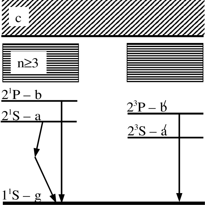
Figure 1: Model energy level diagram for the HeI atom used here.

The estimates made by Zeldovich et al. (1968) and Peebles (1968) and subsequently confirmed by numerical calculations using multilevel model atoms (Grachev and Dubrovich 1991; Seager et al. 2000) showed that a simplified recombination model (the so-called three-level model; Zeldovich et al. 1968; Peebles 1968; Matsuda et al. 1969; Seager et al. 1999) could be used to calculate the ionization fraction as a function of time. In this model, the recombination rate for helium (the model energy level diagram is presented in Fig. 1) is determined by the following processes: the two-photon $2^{1}S\rightarrow 1^{1}S$ transitions and the one-photon $2^{1}P\rightarrow 1^{1}S$ and $2^{3}P\rightarrow 1^{1}S$, i.e., three terms remain in sum (2) and the following formula is valid:

$$J_{tot}\simeq J_{ag}+J_{bg}+J_{b^{\prime}g}$$ (4)

where the subscripts denote the following states: $g\equiv 1^{1}S$, $a\equiv 2^{1}S$, $b\equiv 2^{1}P$, $b^{\prime}\equiv 2^{3}P$ (see Fig. 1).

A proper allowance for the resonance transitions requires a joint analysis of the kinetics of transitions and radiative transfer in the $2^{1}P\rightarrow 1^{1}S$ and $2^{3}P\rightarrow 1^{1}S$ lines by including a number of peculiar factors, with the cosmological expansion and the absorption of HeI resonance photons by neutral hydrogen (HI) being the most important of them.

According to Eq. (3), the two-photon HeI $2^{1}S\rightarrow 1^{1}S$ transition rate can be calculated using the formula (for convenience, the common factor was taken out of the brackets):

$$J_{ag}=A_{ag}\left(N_{a}-{g_{a}\over g_{g}}\eta^{0}_{ag}N_{g}\right)$$ (5)

where $A_{ag}=51.3$ с^-1 is the coefficient of the spontaneous two-photon $2^{1}S\rightarrow 1^{1}S$ decays, $N_{a}$ [cm^-3] is the population of the $2^{1}S$ state, $N_{g}$ [cm^-3] is the population of the $1^{1}S$ state, $g_{a}=1$ is the statistical weight of the $2^{1}S$ state, $g_{g}=1$ is the statistical weight of the $1^{1}S$ state, $\eta^{0}_{ag}$ is the equilibrium photon occupation number at the $2^{1}S\rightarrow 1^{1}S$ ($a\rightarrow g$) transition frequency.

For optically thick transitions (for HeI at the HeII$\rightarrow$HeI recombination epoch, these are the $n^{1}P\rightarrow 1^{1}S$ and $2^{3}P\rightarrow 1^{1}S$ transitions and, when the three-level model is used, the $b\rightarrow g$ and $b^{\prime}\rightarrow g$ transitions, respectively) the rates of the direct and reverse processes appearing in Eq. (3) are very close (their relative difference can reach $10^{-9}$, depending on n and the instant of time under consideration), because the occupation numbers of the photon field in HeI lines (including both equilibrium and intrinsic HeI recombination radiations) are close to their quasi-equilibrium values, $\eta_{fg}\simeq N_{n}/g_{n}N_{1}$.

Thus, if $J_{n1}$ are calculated from Eq. (3), then two relatively close numbers often has to be subtracted. In this case, a significant loss of the computation accuracy is possible (Burgin 2003). Therefore, the following formula that is devoid of the above shortcoming is used to consider the kinetics of such optically thick transitions:

$$J_{fg}=P_{fg}A_{fg}\left(N_{f}-{g_{f}\over g_{g}}\eta^{0}_{fg}N_{g}\right)$$ (6)

where the subscript $f$ denotes the $nP$ state, $A_{fg}$ is the Einstein coefficient for the spontaneous $f\rightarrow g$ transition, $N_{f}$ is the population of state $f$, and $g_{f}$ is the statistical weight of state $f$. The quantity $P_{fg}$ is the probability of the uncompensated $f\leftrightarrow g$ transitions.

The quantity $P_{fg}$ can be calculated by jointly considering the radiative transfer equation in the $f\rightarrow g$ line and the balance equation for levels $f$ and $g$. It contains information about the effect of the intrinsic resonance plasma radiation on the transition kinetics with allowance made for the circumstances that accompany the radiative transfer, such as the cosmological expansion, the absorption of HeI resonance photons by neutral hydrogen, etc.

Since the $f\rightarrow g$ transition rate $J_{fg}$, which, in turn, determines the recombination rate $J_{tot}$, directly depends on $P_{fg}$, a proper calculation of $P_{fg}$ for the primordial plasma conditions is one of the most important subgoals of the cosmological recombination theory.

The methods for including $P_{fg}$ in the multilevel code that computes the kinetic equations for the full system of levels can be found in Seager et al. (2000), Switzer and Hirata (2008), and Rubino-Martin et al. (2007). The kinetic equation that describes the HeII$\rightarrow$HeI recombination in terms of the simplified model and the methods for including $P_{fg}$ in it can be found in KhIV07 and Wong et al. (2008).

3 Kinetics of HeI 2P$\rightarrow$1S resonance transitions

Let us consider the HeI $f\rightarrow g$ resonance transition kinetics using HeI 2P$\rightarrow$1S (i.e. $b\rightarrow g$ and $b^{\prime}\rightarrow g$), which mainly determine the recombination rate $J_{tot}$, as an example. A joint analysis of the balance equation for levels $f$ and $g$ and the radiative transfer equation for the HeI $f\rightarrow g$ line leads to the following formula for the probability of the uncompensated $f\rightarrow g$ transitions:

$$P_{fg}=\int_{0}^{\infty}{\kappa_{H}+\kappa_{He,f}\exp\left(-\tau_{f}\right)\over\kappa_{H}+\kappa_{He,f}}\psi_{fg}(\nu)d\nu$$ (7)

where $\kappa_{H}$ [cm^-3s^-1Hz^-1] is the absorption coefficient of photons ($h\nu\geq 13.6$ eV) by neutral hydrogen during ionization, $\kappa_{He,f}$ is the absorption coefficient of photons by neutral helium in the $f\rightarrow g$ line, $\tau_{f}$ is the optical depth for the absorption of HeI resonance photons (including the absorption by both helium and hydrogen atoms), and $\psi_{fg}(\nu)$ is the emission profile in the HeI $f\rightarrow g$ line ($\int\psi_{fg}(\nu)d\nu=1$).

The coefficient $\kappa_{H}$ is given by the formula

$$\kappa_{H}={8\pi\nu^{2}\over c^{2}}\sigma_{H}(\nu)N_{H,1S}$$ (8)

where $\sigma_{H}(\nu)$ is the photoionization cross section of the HI ground state by a photon with frequency $\nu$, $N_{H,1S}$ is the number density of hydrogen atoms in the ground state, which is equal, with a good accuracy, to the neutral hydrogen number density $N_{HI}$.

The coefficient $\kappa_{He,f}$ ($f=b$ or $b^{\prime}$) is given by the formula:

$$\kappa_{He,f}={g_{f}\over g_{g}}A_{fg}N_{g}\phi_{fg}(\nu)$$ (9)

where $\phi_{fg}(\nu)$ is the absorption profile in the HeI $f\rightarrow g$ line ($\int\phi_{fg}(\nu)d\nu=1$). The ground-state population $N_{g}$ is equal, with a good accuracy, to the total neutral helium number density $N_{HeI}$.

The optical depth $\tau_{f}$ is given by the formula

$$\tau_{f}(\nu,z)=\int_{\nu}^{\infty}{{c^{3}\over 8\pi\nu^{\prime 3}}H^{-1}(z^{\prime})\left(\kappa_{H}(\nu^{\prime},z^{\prime})+\kappa_{He,f}(\nu^{\prime},z^{\prime})\right)}d\nu^{\prime}$$ (10)

where $H(z)=H_{0}\sqrt{\Omega_{\Lambda}+\Omega_{m}(1+z)^{3}+\Omega_{rel}(1+z)^{4}}$ is the Hubble constant (the parameters $H_{0},\leavevmode\nobreak\ \Omega_{\Lambda},\leavevmode\nobreak\ \Omega_{m},\leavevmode\nobreak\ \Omega_{rel}$ are described below in Table LABEL:cosm_par), and the parameter $z^{\prime}$ is defined by the equality $z^{\prime}=(1+z)\nu^{\prime}/\nu-1$.

For the convenience of the subsequent consideration, let us represent $P_{fg}$ as the sum of two terms: $P_{fg}=P^{H}_{fg}+P^{red}_{fg}$, where $P^{H}_{fg}$ and $P^{red}_{fg}$ are given by the formulas:

$$P^{H}_{fg}=\int_{0}^{\infty}{\kappa_{H}\over\kappa_{H}+\kappa_{He,f}}\psi_{fg}(\nu)d\nu$$ (11)

$$P^{red}_{fg}=\int_{0}^{\infty}{\kappa_{He,f}\exp\left(-\tau_{f}\right)\over\kappa_{H}+\kappa_{He,f}}\psi_{fg}(\nu)d\nu$$ (12)

The quantity $P^{H}$ is the mean (averaged over the profile $\psi_{fg}(\nu)$) destruction probability of a HeI $f\rightarrow g$ resonance photon as a result of its interaction with neutral hydrogen.

The quantity $P^{red}_{fg}$ is the escape probability of HeI $f\rightarrow g$ photons from the line profile due to the cosmological expansion. Note that the definition of this quantity differs from the classical definition of the Sobolev photon escape probability from the line profile $P^{S}_{fg}$ (Rybicki and dell Antonio 1993; Seager et al. 2000), being its generalization to the case that includes the absorption of HeI resonance photons by neutral hydrogen (in this sense, $P^{red}_{fg}$ may be called a modified photon escape probability from the line profile). If the absorption of HeI resonance photons by neutral hydrogen is negligible (i.e., $\kappa_{H}/\kappa_{He,f}\ll 1$), then the formula for $P^{red}_{fg}$ takes the classical form:

$$P^{red}_{fg}|_{\kappa_{H}=0}=\int_{0}^{\infty}\exp\left(-\tau_{He,f}(\nu)\right)\psi_{fg}(\nu)d\nu\simeq P^{S}_{fg}\equiv\tau_{He,f}^{-1}\left(1-\exp\left(-\tau_{He,f}\right)\right)$$ (13)

where $\tau_{He,f}(\nu)$ is the optical depth for photon absorption in the HeI $f\rightarrow g$ line as a function of the frequency and $\tau_{He,f}$ is the total optical depth for photon absorption in the HeI $f\rightarrow g$ line given by the formula:

$$\tau_{He,f}={g_{f}A_{fg}N_{g}c^{3}\over g_{g}8\pi H\nu_{fg}^{3}}\;.$$ (14)

Note that Switzer and Hirata (2008) and Rubino-Martin et al. (2007) used a different splitting into terms, namely, $P_{fg}=P^{S}_{fg}+\Delta P^{esc}_{fg}$, where $\Delta P^{esc}_{fg}$ is the correction to the Sobolev escape probability due to the presence of continuum absorption.

3.1 The Modified Photon Escape Probability from the Line Profile

Using (9) and (10), we can transform Eq. (12) to

$$P^{red}_{fg}={g_{g}\over g_{f}A_{fg}N_{g}}\int_{0}^{\tau_{f}}\left({\kappa_{He,f}\over\kappa_{H}+\kappa_{He,f}}\right)^{2}\left({\psi_{fg}(\nu)\over\phi_{fg}(\nu)}\right){8\pi\nu^{3}H\over c^{3}}\exp\left(-\tau^{\prime}\right)d\tau^{\prime}$$ (15)

This integral can be roughly estimated from the formula

$$P^{red}_{fg}=\left(1+\gamma^{-1}\right)^{-2}\tau_{He,f}^{-1}\left(1-\exp\left(-\tau_{He,f}\right)\right)$$ (16)

where the parameter $\gamma$ is the ratio of the helium and hydrogen absorption coefficients at the central frequency of the $f\rightarrow g$ line and is given by the expression:

$$\gamma\equiv{k_{He}(\nu_{fg})\over k_{H}(\nu_{fg})}={\left(g_{f}/g_{g}\right)A_{fg}N_{HeI}\phi_{fg}(\nu_{fg})c^{2}\over\sigma_{H}\left(\nu_{fg}\right)8\pi\nu_{fg}^{2}N_{HI}}$$ (17)

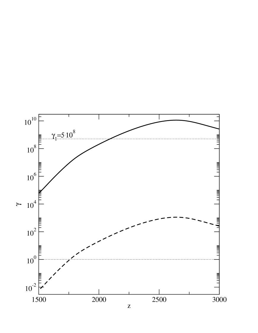
Figure 2: Ratio of the HeI and HI absorption coefficients at the central frequency of the $f\rightarrow g$ line ($\gamma$) versus redshift $z$ for the HeI $2^{1}P\rightarrow 1^{1}S$ (solid curve) and HeI $2^{3}P\rightarrow 1^{1}S$ (dashed curve) transitions. The dotted straight lines indicate the unit and $\gamma_{1}=5\cdot 10^{8}$ levels. The value of $\gamma_{1}=5\cdot 10^{8}$ is explained in the text.

The $z$ dependence of $\gamma$ for the $2^{1}P\rightarrow 1^{1}S$ and $2^{3}P\rightarrow 1^{1}S$ transitions is presented in Fig. 2.

If the amount of neutral hydrogen is negligible (so that $\gamma\ll 1$) then Eq. (16), as has been noted above, transforms into the standard expression for the Sobolev photon escape probability from the line profile $P^{S}_{fg}$ - (13). If there is much neutral hydrogen (so that $\gamma\gtrsim 1$), then the value of $P^{red}_{fg}$ is lower than the typical Sobolev value of $P^{S}_{fg}$, calculated from (13). In KhIV07, the factor $\left(1+\gamma^{-1}\right)^{-2}$ in Eq. (16) was discarded (i.e., in fact, Eq. (13))was used). For the HeI $2^{1}P\rightarrow 1^{1}S$ transition this neglect is valid throughout the HeII$\rightarrow$HeI recombination epoch, because the values of $\gamma$ for this transition are large (see Fig. 2). For the HeI $2^{3}P\rightarrow 1^{1}S$ transition, this neglect is valid at the early HeII$\rightarrow$HeI recombination epoch ($z\gtrsim 1900$), when the values of $\gamma$ for this transition are large ($\gtrsim 10$, see Fig. 2). At the late HeII$\rightarrow$HeI recombination epoch ($z\lesssim 1750$), when the values of $\gamma$ for the HeI $2^{3}P\rightarrow 1^{1}S$ transition are small ($\lesssim 1$, see Fig. 2), the classical expression for the probability of the uncompensated transitions (13) is inapplicable for the HeI $2^{3}P\rightarrow 1^{1}S$ transitions. At the same time, however, the $2^{1}P\rightarrow 1^{1}S$ transition rate $J_{bg}$, which directly depends on the product $A_{bg}P^{H}_{bg}$, is so large that it completely determines the recombination rate $J_{tot}$. Therefore, the accuracy of calculating $P^{red}_{b^{\prime}g}$ (and, accordingly, the $2^{3}P\rightarrow 1^{1}S$ transition rate $J_{b^{\prime}g}$) does not play significant role.

3.2 The Destruction Probability of a HeI Resonance Photon during Its Interaction with Neutral Hydrogen

The integral expression (11) for $P^{H}$ can be transformed to the following form convenient for both numerical and approximate analytical integrations:

$$P^{H}_{fg}(\gamma)\simeq\int_{0}^{\infty}{\psi_{fg}(\nu)\over 1+\left(\phi_{fg}(\nu)/\phi_{fg}(\nu_{fg})\right)\gamma}d\nu$$ (18)

A further refinement of the form of the function $P^{H}(\gamma)$ depends on the approximation in which the absorption profile $\phi_{fg}(\nu)$ is taken into account and, even more importantly, on the specific form of the emission profile $\psi_{fg}(\nu)$ determined by the physical conditions under which the radiation is scattered and transferred in the $f\rightarrow g$ resonance line.

3.2.1 Complete redistribution in frequency: The Doppler profile

In the case of scattering with a complete redistribution in frequency, if the Doppler profile is used as the absorption, $\phi_{fg}(\nu)$, and emission, $\psi_{fg}(\nu)$, profiles (as was done in KhIV07)), the expression for $P^{H}_{fg}$ takes the form:

$$P^{H}_{D}(\gamma)=\int_{-\infty}^{\infty}{\pi^{-1/2}\exp\left(-y^{2}\right)\over 1+\gamma\exp\left(-y^{2}\right)}dy$$ (19)

where the subscript $D$ stands for ‘‘Doppler’’, while the subscripts $f$ and $g$ were omitted, since the function $P^{H}_{D}(\gamma)$ is universal for all resonance transitions when the Doppler profile is used. This function can be approximated by the expression

$$P^{H}_{D}(\gamma)=\left(1+p\gamma^{q}\right)^{-1}$$ (20)

where the parameters $p,q$ depend on the $\gamma$ range. Their values are given in Table LABEL:tab_pq.

Table 1: Parameters of the approximation of $P^{H}_{D}$

Range of $\gamma$	p	q
$0\leq\gamma\leq 5\cdot 10^{2}$	0.66	0.9
$5\cdot 10^{2}<\gamma\leq 5\cdot 10^{4}$	0.515	0.94
$5\cdot 10^{4}<\gamma\leq 5\cdot 10^{5}$	0.416	0.96
$5\cdot 10^{5}<\gamma$	0.36	0.97

The asymptotics of $P^{H}_{D}(\gamma)$ for $\gamma\rightarrow\infty$ is given by the expression (see, e.g., Ivanov 1969):

$$P^{H}_{D}(\gamma)\simeq{2\over\sqrt{\pi}}\gamma^{-1}\sqrt{\ln{\gamma}}$$ (21)

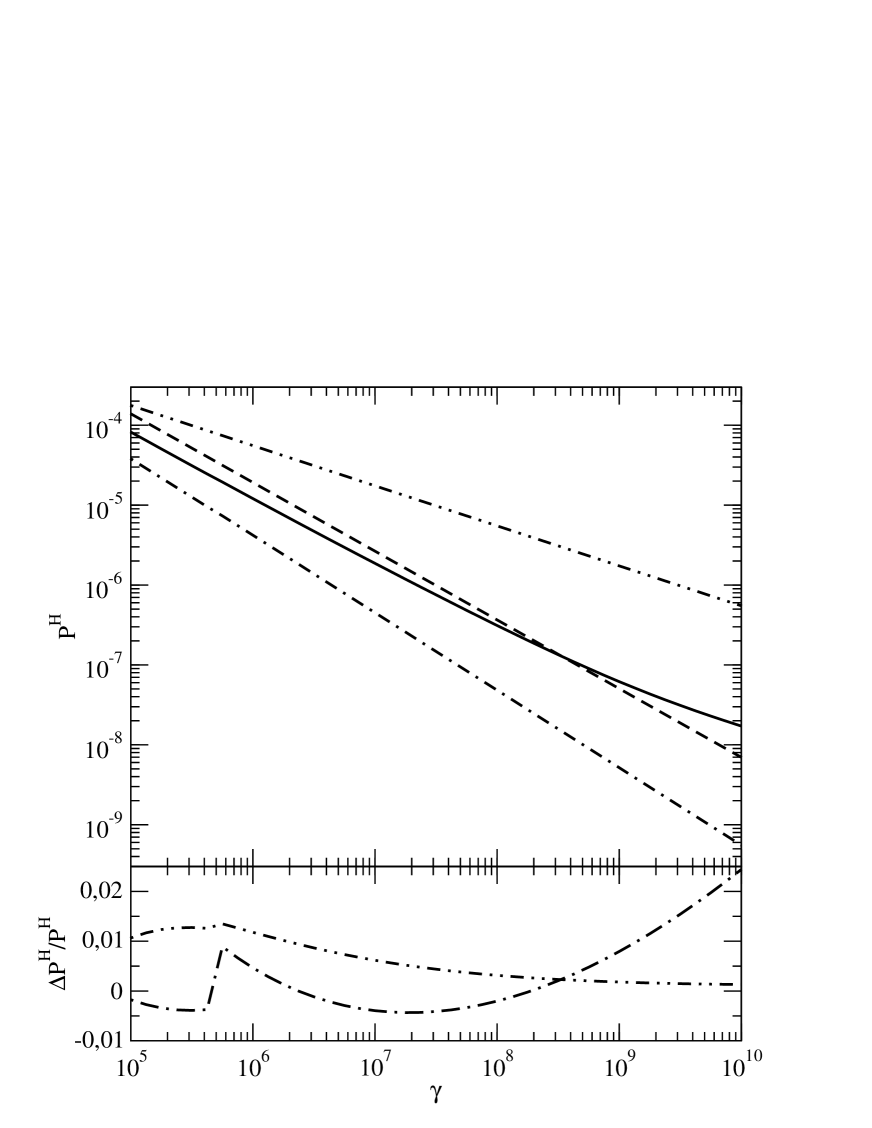
Figure 3: Top panel: Destruction probability of a HeI $2^{1}P\rightarrow 1^{1}S$ resonance photon as it interacts with neutral hydrogen $P^{H}$ versus $\gamma$ for various models of absorption and redistribution in frequency in the HeI $2^{1}P\rightarrow 1^{1}S$ line: the dash-dotted curve corresponds to the use of the Doppler absorption profile, the solid curve corresponds to a partial redistribution in frequency (Eq. (35)), the dashed curve represents the Wong-Moss-Scott approximation, and the dashed curve with two dots corresponds to the use of the Voigt absorption profile for a complete redistribution in frequency. The Voigt parameter is $a=1.7\cdot 10^{-3}$, and the single-scattering albedo is defined by the relation $(1-\lambda)=2.5\cdot 10^{-3}$. Bottom panel: The relative error in $P^{H}$ when calculated from the approximate formulas (22) (the dashed curve with two dots corresponding to the use of the Voigt absorption profile for a complete redistribution in frequency) and (20) (the dash-dotted curve corresponding to the use of the Doppler absorption profile) compared to the numerical calculation based on the exact formula (18).

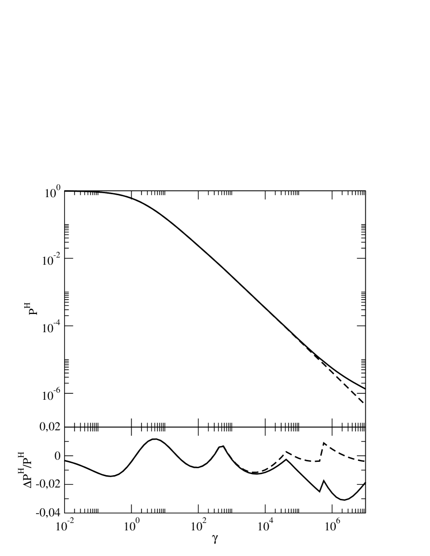
Figure 4: Top panel: Destruction probability of a HeI $2^{3}P\rightarrow 1^{1}S$ resonance photon as it interacts with neutral hydrogen $P^{H}$ versus $\gamma$ for various absorption profiles in the HeI $2^{3}P\rightarrow 1^{1}S$ line: the dashed curve corresponds to the use of the Doppler absorption profile and the solid curve corresponds to the use of the Voigt absorption profile for a complete redistribution in frequency. The Voigt parameter is $a=10^{-5}$ and the single-scattering albedo is approximately equal to zero $\lambda\simeq 0$ (typical values for the HeI $2^{3}P\rightarrow 1^{1}S$ transition at the HeII$\rightarrow$HeI recombination epoch). Bottom panel: The relative error in $P^{H}$ when calculated from the approximate formulas (22) (the solid curve corresponding to the use of the Voigt absorption profile for a complete redistribution in frequency) and (20) (the dashed curve corresponding to the use of the Doppler absorption profile) compared to the numerical calculation based on the exact formula (18).

The results of the calculations of the function $P^{H}_{D}(\gamma)$ for various $\gamma$ ranges are presented in Figs. 3 and 4.

3.2.2 Complete redistribution in frequency: The Voigt profile

In the case of scattering with a complete redistribution in frequency, if the Voigt profile is used as the absorption, $\phi_{fg}(\nu)$ and emission, $\psi_{fg}(\nu)$ profiles, the probability $P^{H}$ can be approximately calculated from the formula

$$P^{H}_{V}\simeq P^{H}_{D}+P^{H}_{W}$$ (22)

where the subscript $V$ stands for ‘‘Voigt’’. The quantity $P^{H}_{W}$ is attributable to the inclusion of the Voigt profile wings (the subscript $W$ stands for ‘‘wings’’) and is given by the formula

$$P^{H}_{W}=2\sqrt{a\over\gamma\pi^{3/2}}\left({\pi\over 2}-\arctan\left(\sqrt{-a_{1}\sqrt{\pi}\ln{a}\over a\gamma}\right)\right)$$ (23)

where $a$ is the Voigt parameter, which is defined by the ratio of the natural (the quantum-mechanical damping constant defining the mean level lifetime) and Doppler widths of level $f$: $a=\Gamma_{f}/4\pi\Delta\nu_{D,f}$, $a_{1}\simeq 1.6$ is an adjustable parameter whose value is chosen from the condition for the best agreement between the values of $P^{H}$ obtained from Eqs. (18) (by numerical integration) and (22). Equation (23) can be derived by taking into account the fact that almost the entire contribution to $\phi_{fg}(\nu)$ at $|\left(\nu-\nu_{fg}\right)/\Delta\nu_{D,f}|\gtrsim|\ln(a)|$ is provided by the Lorentz wings, i.e., the following approximation is valid:

$$\phi_{fg}(\nu)\simeq{a\Delta\nu_{D,f}\over\pi}\left(\nu-\nu_{fg}\right)^{-2}$$ (24)

The thermal width $\Delta\nu_{D,f}$ in Eq. (24) is given by the expression (Lang 1978):

$$\Delta\nu_{D,f}={\nu_{fg}\over c}\sqrt{{2k_{B}T\over m_{He}}+{2\over 3}V_{t}^{2}}$$ (25)

where $m_{He}$ is the helium atomic mass, $T$ is the temperature of the medium, and $V_{t}$ is the root-meansquare turbulent velocity (if the distribution of turbulent velocities is Maxwellian). In our calculations, we assumed that $V_{t}=0$.

The asymptotics of $P^{H}_{V}(\gamma)$ for $\gamma\rightarrow\infty$ is given by the expression (see, e.g., Ivanov 1969):

$$P^{H}_{V}\simeq\pi^{1/4}a^{1/2}\gamma^{-1/2}$$ (26)

The results of the calculations of the function $P^{H}_{V}(\gamma)$ for the HeI $2^{1}P\rightarrow 1^{1}S$ and $2^{3}P\rightarrow 1^{1}S$ and transitions (and various $\gamma$ ranges) are presented in Figs. 3 and 4 respectively.

3.2.3 Partial redistribution in frequency: The Wong-Moss-Scott approximation

Switzer and Hirata (2008) and Rubino-Martin et al. (2007) showed that a partial (rather than complete) redistribution in frequency occurred at the HeII$\rightarrow$HeI recombination epoch in the HeI $n^{1}P\rightarrow 1^{1}S$ lines. These authors performed a significant fraction of their calculations (in particular, the radiative transfer calculations) numerically. Since the problem under consideration is complex, this is computationally demanding and time-consuming (it takes about one day to compute the radiative transfer in HeI lines for one cosmological model; Rubino-Martin et al. 2007). This approach is too resource-intensive to be used in the three-level recombination model incorporated, in particular, in recfast (Seager et al. 1999; Wong et al. 2008), from which a high speed of computations (no more than a few minutes per cosmological model) is demanded at the required accuracy of about 0.1%. This necessitates seeking for an analytic solution to the problem of radiative transfer in a resonance line in an expanding medium in the presence of continuum absorption or at least a suitable approximation that would describe satisfactorily the results of computations with multilevel codes (Switzer and Hirata 2008; Rubino-Martin et al. 2007). This approximation was found by Wong et al. (2008): based on an approximation formula of form (20), Wong et al. (2008) found that at $p=0.36$ and $q=0.86$ for the probability $P^{H}$ of the uncompensated $2^{1}P\rightarrow 1^{1}S$ transitions (let us denote it by $P^{H}_{WMS}$, where the subscript $WMS$ stands for ‘‘Wong-Moss-Scott’’), the simplified (three-level) model describes well the results of computations with the multilevel code by Switzer and Hirata (2008) for any reasonable cosmological parameters. The values of $p=0.66$ and $q=0.9$ (KhIV07) were used to determine the $2^{3}P\rightarrow 1^{1}S$ transition probability.

The asymptotics of $P^{H}_{WMS}(\gamma)$ for $\gamma\rightarrow\infty$ is given by the expression:

$$P^{H}_{WMS}=0.36\gamma^{-0.86}$$ (27)

The results of the calculations of the function $P^{H}_{WMS}$ are presented in Fig. 3.

3.2.4 Partial redistribution in frequency in the wings: The Chugai-Grachev approximation

The Wong-Moss-Scott approximation cannot be used to investigate the kinetics of HeI $n^{1}P\rightarrow 1^{1}S$ resonance transitions for $n\geq 3$, since the parameters $p$ and $q$ in Eq. (20) should have different values unique for each specific $n$ in this case. This necessitates seeking for an expression for the probability of the uncompensated transitions based on an analytic solution of the radiative transfer equation in the HeI resonance lines at the HeII$\rightarrow$HeI recombination epoch.

Being formulated in full, this problem is very complex, since it requires including a large number of processes, such as the Hubble expansion, the partial redistribution in frequency due to the thermal motion of atoms, the Raman scattering, the continuum absorption, the recoil upon scattering, etc. In this case, the problem requires considering an integrodifferential equation in which the redistribution function cannot be expressed in terms of elementary functions. Therefore, in this formulation, it is solved mainly through computer simulations (Switzer and Hirata 2008; Rubino-Martin et al. 2007). Nevertheless, a number of simplifications and approximations make it possible to reformulate the problem in a form that allows a completely analytic solution. Thus, for example, Chugai (1987) and Grachev (1988) considered the diffusion of resonance line radiation in the presence of continuum absorption. In comparison with the complete formulation of the problem of radiative transfer in a line, these authors disregarded the following effects: (1) the Raman scattering was disregarded; (2) a differential expression derived in the diffusion approximation was used instead of the exact integral term describing the redistribution of photons in frequency due to the thermal motion of atoms (see, e.g., Varshalovich and Sunyaev 1968; Nagirner 2001), i.e., the final equation has the form of a frequency diffusion equation for photons (Harrington 1973; Basko 1978); (3) the Doppler core of the Voigt absorption profile was fitted by a delta function; and (4) when formulating the mathematical model, Grachev (1988) disregarded the expansion of the medium, although Chugai (1987) previously took it into account. Comparison of the papers by Chugai (1987) and Grachev (1988) in this aspect shows that the contributions to the probability of the uncompensated transitions from the expansion of the medium and the continuum absorption can be approximately taken into account independently of each other. Chugai (1987) derived the following formula for the probability of the uncompensated transitions (note that Chugai (1987) and Grachev (1988) used notations differing from each other and from the notation of this paper):

$$P^{H}_{C}=1.217a^{1/4}\gamma^{-3/4}$$ (28)

where the subscript $C$ stands for ‘‘Chugai’’. The functional dependence in Eq. (28) was determined from qualitative considerations, while the numerical coefficient was determined by numerically solving the diffusion equation.

Grachev (1988) analytically derived the formula:

$$P^{H}_{G}=(8\lambda a)^{1/4}\pi^{-5/8}\gamma^{-3/4}F\left({1\over 2},2,s+2,{1\over 2}\right){\Gamma(s+3/2)\over\Gamma(s+2)}$$ (29)

where the subscript $G$ stands for ‘‘Grachev’’, $\lambda$ is the single-scattering albedo, $F$ is the hypergeometric function, $\Gamma$ is the gamma function, and the parameter $s$ is defined by the formula:

$$s=2^{-3/2}\pi^{-1/4}(1-\lambda)\lambda^{-1/2}a^{1/2}\gamma^{1/2}-1/4$$ (32)

Equation (29) has the following asymptotics:
1) at small $\gamma$ ($\gamma\ll\gamma_{1}\equiv\pi^{1/2}\lambda\left(2a(1-\lambda)^{2}\right)^{-1}$):

$$P^{H}_{G}\simeq 1.217(\lambda a)^{1/4}\gamma^{-3/4}$$ (33)

2) at large $\gamma$ ($\gamma\gg\gamma_{1}$)

$$P^{H}_{G}\simeq 2^{3/2}\pi^{-1/2}(1-\lambda)^{-1/2}\lambda^{1/2}\gamma^{-1}$$ (34)

We see that at small $\gamma$ ($\gamma\ll\gamma_{1}$, which corresponds to $\gamma\ll 5\cdot 10^{8}$ for the HeI $2^{1}P\rightarrow 1^{1}S$ transition) and $\lambda$ close to unity, Eq. (33) matches the solution obtained by Chugai (1987).

It should be noted that Eqs. (28) and (29) were derived by Chugai (1987) and Grachev (1988) for $\gamma$ at which $a\gamma\gg 1$ and cannot be applied at $a\gamma\lesssim 1$. This can be seen from the following: 1) when $\gamma\rightarrow 0$, $P^{H}_{C}$ and $P^{H}_{G}$ tend to infinity; 2) when the Voigt parameter tends to zero ($a\rightarrow 0$), $P^{H}_{C}$ and $P^{H}_{G}$ also tend to zero, while the probability $P^{H}$ that they describe tends to $P^{H}_{D}$ that corresponds to the correct description of the Doppler core (in terms of the Doppler profile rather than the delta function, as was done by Chugai (1987) and Grachev (1988)). It should also be noted that the correct description of the Doppler core leads to a correction of about 10% to $P^{H}_{G}$ for the HeI $2^{1}P\rightarrow 1^{1}S$ transition in the range $10^{6}\leq\gamma\leq 10^{9}$.

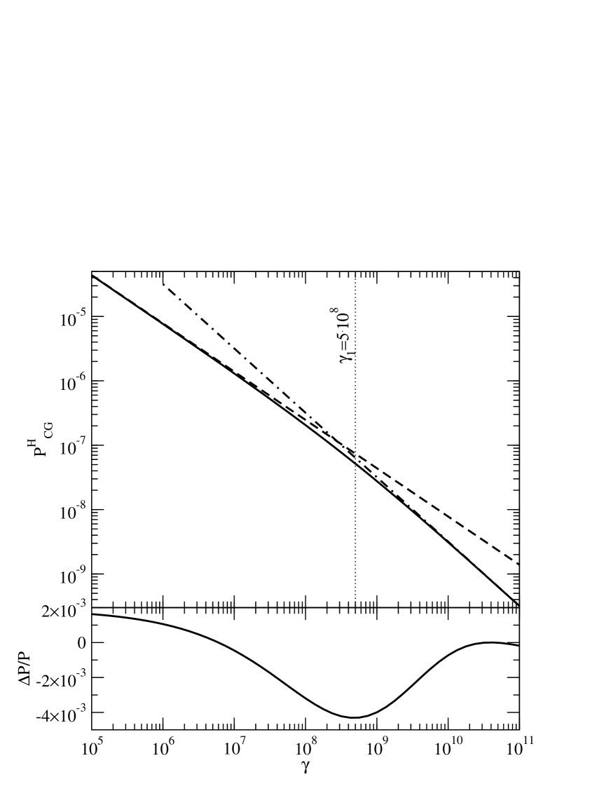
Figure 5: Top panel: Destruction probability of a HeI $2^{1}P\rightarrow 1^{1}S$ resonance photon as it interacts with neutral hydrogen $P^{H}_{G}$ (29) versus $\gamma$ (solid curve), asymptotics (33) corresponding to $\gamma\ll\gamma_{1}$ (dashed curve) (Chugai 1987; see the text), and asymptotics (34) corresponding to $\gamma\gg\gamma_{1}$ (dash-dotted curve). The Voigt parameters is $a=1.7\cdot 10^{-3}$ and the single-scattering albedo is defined by the relation $(1-\lambda)=2.5\cdot 10^{-3}$ (typical values for the HeI $2^{1}P\rightarrow 1^{1}S$ transition at the HeII$\rightarrow$HeI recombination epoch). Bottom panel: The relative error in $P^{H}_{G}$ approximately calculated from Eqs. (30) and (31) compared to the calculations based on Eq. (29).

The results of the calculations of the function $P^{H}_{G}$, its asymptotics (33) and (34), and the relative error in $P^{H}_{G}$ calculated from the approximation formulas (30) and (31) compared to the calculations based on the exact formula (29) are presented in Fig. 5. Comparison of asymptotics (33) and (34) (Fig. 5) shows that the $\gamma$ dependence of $P^{H}_{G}$, changes significantly at $\gamma$ close to $\gamma_{1}$ (e.g., on a logarithmic scale, the slope $\partial\ln{P^{H}_{G}}/\partial\ln{\gamma}$ changes from -0.75 to -1). This should be taken into account when the Chugai-Grachev approximation is used to calculate the HeII$\rightarrow$HeI recombination kinetics, because $\gamma$ (for the HeI $2^{1}P\rightarrow 1^{1}S$ transition) takes on values close to $\gamma_{1}\sim 5\cdot 10^{8}$ during the HeII$\rightarrow$HeI recombination (at the epochs $z=1900-2100$) (see Fig. 2).

3.2.5 Partial redistribution in frequency: An approximate allowance for the Raman scattering

Since Chugai (1987) and Grachev (1988) (1) disregarded the Raman scattering and (2) described the central region of the absorption profile by $\delta$-function, Eq. (29) gives an underestimated value compared to the probability $P^{H}$, determined when solving the full problem, in which the Raman scattering contributing to the formation of broader wings in the emission profile $\psi_{fg}(\nu)$, is taken into account and the central region of the absorption profile (Doppler core) is described by the Voigt profile. To estimate the contribution from the Raman scattering and the Doppler core to the probability of the uncompensated transitions $P^{H}$, let us represent Eq. (18) as:

$$P^{H}\simeq P^{H}_{D}+P^{H}_{G}+P^{H}_{R}$$ (35)

where $P^{H}_{D}$, $P^{H}_{G}$ and $P^{H}_{R}$ are the contributions to the probability $P^{H}$, from various physical effects. These quantities are explained in detail below.

1) The contribution $P^{H}_{D}$ can be defined by the formula:

$$P^{H}_{D}=\int_{A}{\psi_{fg}(\nu)\over 1+\left(\phi_{fg}(\nu)/\phi_{fg}(\nu_{fg})\right)\gamma}d\nu\;,\leavevmode\nobreak\ \leavevmode\nobreak\ \leavevmode\nobreak\ \leavevmode\nobreak\ \leavevmode\nobreak\ \leavevmode\nobreak\ \leavevmode\nobreak\ \leavevmode\nobreak\ A\simeq[\nu_{fg}-3\Delta\nu_{D};\nu_{fg}+3\Delta\nu_{D}]$$ (36)

where $A$ is the Doppler core region. The quantity $P^{H}_{D}$ includes the contribution from the absorption of HeI resonance photons from the Doppler core region to the probability of the uncompensated HeI $2^{1}P\rightarrow 1^{1}S$, which is disregarded in the Chugai-Grachev approach. The quantity $P^{H}_{D}$ can be calculated using Eq. (20).

2) The contribution $P^{H}_{G}$ can be defined by the formula:

$$P^{H}_{G}=\int_{B}{\psi_{fg}(\nu)\over 1+\left(\phi_{fg}(\nu)/\phi_{fg}(\nu_{fg})\right)\gamma}d\nu\;,\leavevmode\nobreak\ \leavevmode\nobreak\ \leavevmode\nobreak\ \leavevmode\nobreak\ \leavevmode\nobreak\ \leavevmode\nobreak\ \leavevmode\nobreak\ \leavevmode\nobreak\ B\simeq[\nu_{fg}-\nu_{CG};\nu_{fg}-3\Delta\nu_{D}]\cup[\nu_{fg}+3\Delta\nu_{D};\nu_{fg}+\nu_{CG}]$$ (37)

The quantity $P^{H}_{G}$ includes the contribution from the region of the ‘‘near’’ wings $B$, where the redistribution in frequency due to the thermal motion of atoms plays a crucial role in forming the emission profile, just as in the Doppler core region. $P^{H}_{G}$ can be calculated using Eq. (29). The characteristic frequency $\nu_{CG}$ specifies the boundaries of the frequency region $B$ in such a way that the redistribution in frequency due to the thermal motion of atoms considered by Chugai (1987) and Grachev (1988) has a decisive effect on the formation of the emission profile in the frequency range $[\nu_{fg}-\nu_{CG};\nu_{fg}+\nu_{CG}]$, while the Raman scattering has a decisive effect on the formation of the emission profile in the frequency ranges $[0;\nu_{fg}-\nu_{CG}]$ and $[\nu_{fg}+\nu_{CG};\infty]$. We calculate $\nu_{CG}$ below.

3) The contribution $P^{H}_{R}$ can be defined by the formula:

$$P^{H}_{R}=\int_{C}{\psi_{fg}(\nu)\over 1+\left(\phi_{fg}(\nu)/\phi_{fg}(\nu_{fg})\right)\gamma}d\nu\;,\leavevmode\nobreak\ \leavevmode\nobreak\ \leavevmode\nobreak\ \leavevmode\nobreak\ \leavevmode\nobreak\ \leavevmode\nobreak\ \leavevmode\nobreak\ \leavevmode\nobreak\ C\simeq[0;\nu_{fg}-\nu_{CG}]\cup[\nu_{fg}+\nu_{CG};\infty]$$ (38)

The quantity $P^{H}_{R}$ includes the contribution from the region of the ‘‘far’’ wings $C$, where the Raman scattering (the subscript $R$ stands for ‘‘Raman’’) plays a crucial role in forming the emission profile.

Since the emission and true absorption profiles in the ranges of integration in (38) are defined by the expressions $\psi_{fg}(\nu)=(1-\lambda)\phi_{V}(\nu)$, and $\phi_{fg}(\nu)=(1-\lambda)\phi_{V}(\nu)$ (where $\phi_{V}(\nu)$ is the Voigt profile), we obtain

$$P^{H}_{R}=2(1-\lambda)\sqrt{a\over(1-\lambda)\gamma\pi^{3/2}}\left({\pi\over 2}-\arctan\left(f(a,\lambda,\gamma)\right)\right)$$ (39)

where $f(a,\lambda,\gamma)$ is defined by the expression

$$f(a,\lambda,\gamma)=A_{1}\pi^{1/4}\left((1-\lambda)a\gamma\right)^{-1/2}\left({\nu_{CG}\over\Delta\nu_{D}}\right)$$ (40)

Here, $A_{1}$ is the correction factor that takes into account the fact that the two effects (both the redistribution in frequency due to the thermal motion of atoms and the Raman scattering) give comparable contributions to the probability $P^{H}$ at frequencies close to the boundary frequency $\nu_{fg}-\nu_{CG}$ (and, accordingly, $\nu_{fg}+\nu_{CG}$) (i.e., there is no well-defined boundary between the zones of influence of these effects).

Using the results by Chugai (1987) and Grachev (1988), one can show that the integrand in (35) in the central frequency region $[\nu_{fg}-\nu_{CG};\nu_{fg}+\nu_{CG}]$ depends on the frequency as

$${\psi_{fg}(\nu)\over 1+\left(\phi_{fg}(\nu)/\phi_{fg}(\nu_{fg})\right)\gamma}\sim\exp\left(-{\left(x\over 2^{1/4}\pi^{-1/8}(\lambda a\gamma)^{1/4}\right)^{2}}\right)$$ (41)

where $x=(\nu-\nu_{fg})/\Delta\nu_{D}$.

In the frequency ranges $[0;\nu_{fg}-\nu_{CG}]$ and $[\nu_{fg}+\nu_{CG};\infty]$, where the effect of Raman scattering prevails, the integrand in (35) depends on the frequency as

$${\psi_{fg}(\nu)\over 1+\left(\phi_{fg}(\nu)/\phi_{fg}(\nu_{fg})\right)\gamma}\sim{a(1-\lambda)\over\pi x^{2}+a(1-\lambda)\gamma\sqrt{\pi}}$$ (42)

Comparing Eqs. (41) and (42), we can find the characteristic frequency $\nu_{CG}$ in the form

$$\nu_{CG}\simeq 2^{1/4}\pi^{-1/8}(\lambda a\gamma)^{1/4}\sqrt{\ln{\gamma}}\Delta\nu_{D}$$ (43)

Substituting (43) into (40), we obtain the final expression for $f(a,\lambda,\gamma)$:

$$f(a,\lambda,\gamma)\simeq A_{1}2^{1/4}\pi^{1/8}(1-\lambda)^{-1/2}\lambda^{1/4}\left(a\gamma\right)^{-1/4}\sqrt{\ln{\gamma}}$$ (44)

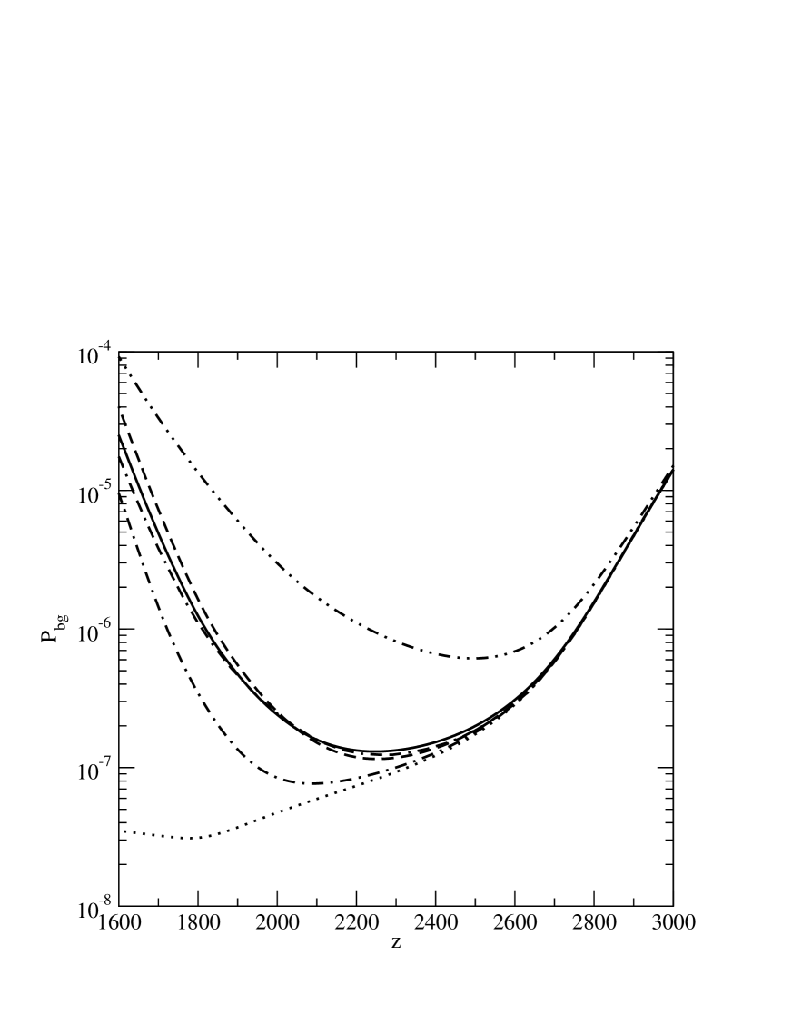
Figure 7: Probability of the uncompensated HeI $2^{1}P\rightarrow 1^{1}S$ transitions $P_{bg}$ versus redshift $z$ for various models of absorption and redistribution in frequency in HeI $2^{1}P\rightarrow 1^{1}S$ line: the dash-dotted curve corresponds to the use of the Doppler absorption profile, the solid curve represents a partial redistribution in frequency (this paper), the dash-dash-dot curve represents a partial redistribution in frequency (Rubino-Martin et al. 2007), the dashed curve represents the Wong-Moss-Scott approximation, the dashed curve with two dots corresponds to the use of the Voigt absorption profile for a complete redistribution in frequency, and the dotted curve represents the Sobolev probability $P^{S}_{bg}$ (calculated from Eq. (13)). The curves were calculated for the cosmological parameters adopted in Rubino-Martin et al. (2007).

The coefficient $A_{1}=0.5$ can be determined from the condition for the best agreement between the dependences $P_{bg}(z)=(P^{red}_{bg}(z)+P^{H}_{bg}(z))$ (see Fig. 7), calculated here and in Rubino-Martin et al. (2007).

It should be noted that we assume here that if the fraction of coherent scatterings (i.e., the singlescattering albedo) is equal to $\lambda$, then the fraction of Raman scatterings is equal to $(1-\lambda)$, i.e., only the radiative transitions are taken into account, while the effect of the transitions produced by electron collisions is considered negligible. This approximation is valid at the HeII$\rightarrow$HeI recombination epoch. In the general case where the effect of electron collisions is not negligible, the fraction of Raman scatterings is not equal to $(1-\lambda)$. This should be taken into account when the above formulas are used.

As the fraction of coherent scatterings $\lambda$ changes, Eq. (35) has the following asymptotics:
1) As the fraction of coherent scatterings $\lambda$ tends to unity, Eq. (35) turns into the sum of $P^{H}_{D}$ and $P^{H}_{C}$ given by Eq. (28) (Chugai 1987). This limit corresponds to the absence of Raman scatterings, i.e., the resonance photons are redistributed in frequency solely through the thermal motion of atoms.
2) As the fraction of coherent scatterings $\lambda$ tends to zero, Eq. (35) tends to $P^{H}_{V}$ given by Eq. (22). This limit corresponds to a completely incoherent scattering, which leads to a complete redistribution of resonance photons in frequency. As a result, the Voigt emission profile is formed.

4 The Cosmological Model

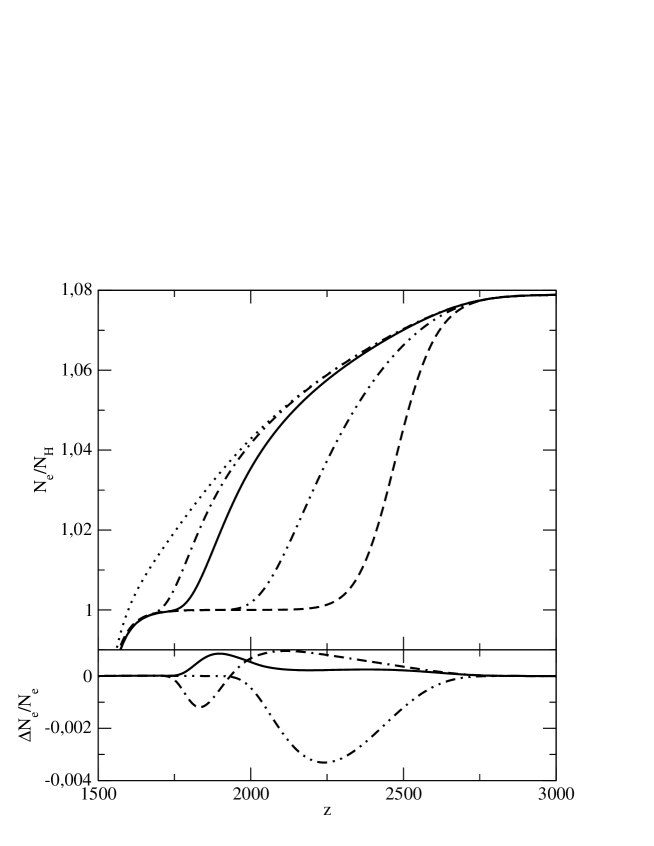
Figure 6: Top panel: Relative number of free electrons $N_{e}/N_{H}$ versus redshift $z$: the dashed curve represents the equilibrium recombination, the dotted curve represents the recombination according to the model without any absorption of HeI resonance photons by neutral hydrogen; the dash-dotted curve represents the recombination according to the model by KhIV07; the solid curve represents the recombination according to this work (Eqs. (22) and (35) describe the HeI $2^{3}P\rightarrow 1^{1}S$ and HeI $2^{1}P\rightarrow 1^{1}S$ transition probabilities, respectively); the dashed curve with two dots represents the recombination calculated using the approximation of a complete redistribution in frequency in HeI resonance lines (Eq. (22) describes the probability of both HeI $2^{3}P\rightarrow 1^{1}S$ and HeI $2^{1}P\rightarrow 1^{1}S$ transitions). All curves were calculated for the cosmological parameters adopted in Rubino-Martin et al. (2007). Bottom panel: The relative difference in the fraction of free electrons for different recombination models: the solid curve indicates the difference between our results and the results by Rubino-Martin et al. (2007) for the models with a partial redistribution in frequency; the dashed curve with two dots indicates the difference between our results and the results of Rubino-Martin et al. (2007) for the models with a complete redistribution in frequency; the dash-dash-dot curve indicates the difference between the results based on the model by Wong et al. (2008) and those by Rubino-Martin et al. (2007) for the model with a partial redistribution in frequency.

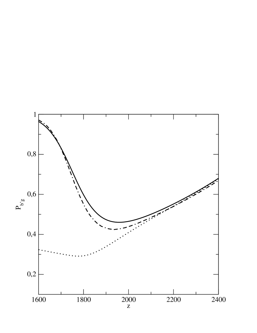
Figure 8: Probability of the uncompensated HeI $2^{3}P\rightarrow 1^{1}S$ transitions $P_{b^{\prime}g}$ versus redshift $z$: the solid curve represents our result (Eq. (22) was used for the calculations, which corresponds to the use of the Voigt absorption profile for a complete redistribution in frequency), the dash-dash-dot curve represents the result by Rubino-Martin et al. (2007), and the dotted curve represents the Sobolev probability $P^{S}_{b^{\prime}g}$ (calculated from Eq. (13)). The curves were calculated for the cosmological parameters adopted in Rubino-Martin et al. (2007).

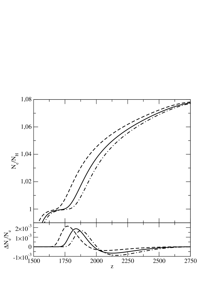
Figure 9: Top panel: Relative number of free electrons $N_{e}/N_{H}$ versus redshift $z$ for various baryonic matter densities: the dashed, solid, and dash-dotted curves correspond to $\Omega_{b}=0.02$, $\Omega_{b}=0.04$, and $\Omega_{b}=0.06$, respectively. The remaining parameters of the cosmological model are given in Table LABEL:cosm_par. Bottom panel: The relative difference in the number density of free electrons between the calculations using our model and those using the model by Wong et al. (2008) (the Wong-Moss-Scott approximation): the dashed, solid, and dash-dotted curves correspond to $\Omega_{b}=0.02$, $\Omega_{b}=0.04$, and $\Omega_{b}=0.06$, respectively.

We performed all calculations within the framework of standard cosmological $\Lambda$CDM models. The calculation results presented in Figs. 6, 7 and 8 were obtained using the cosmological parameters from Rubino-Martin et al. (2007) (since these figures reflect, in particular, the comparison of our results with those of Rubino-Martin et al. (2007)). The results of calculations presented in Fig. 9 were obtained using the cosmological parameters from Table LABEL:cosm_par.

Table 2: Parameters of the standard cosmological model

Description	Designation	Value
Total matter density	$\Omega_{tot}$	1
(in units of critical density)
Baryonic matter density	$\Omega_{b}$	$0.02-0.06$
Nonrelativistic matter density	$\Omega_{m}=\Omega_{CDM}+\Omega_{b}$	$0.27$
Relativistic matter density	$\Omega_{rel}=\Omega_{\gamma}+\Omega_{\nu}$	$8.23\cdot 10^{-5}$
Vacuum-like matter density	$\Omega_{\Lambda}$	$0.73$
Hubble constant	$H_{0}$	70 km/s/Mpc
CMBR temperature today	$T_{0}$	$2.726$ K
Helium mass fraction	$Y$	$0.24$

5 Results and Discussion

The calculated destruction probabilities of resonance photons as they interact with neutral hydrogen $P^{H}$ are plotted against the ratio of the helium and hydrogen absorption coefficients $\gamma$ in Figs. 3 and 4 for various models of photon redistribution in frequency. As we see from these figures, the probabilities $P^{H}$ are lowest and highest when the Doppler and Voigt profiles, respectively, are used to describe the absorption and emission coefficients. This is because the Doppler profile ‘‘has no wings’’, while the Voigt profile has slowly descending Lorentzian wings. Therefore, the calculated $P^{H}$ for any other models of redistribution (for a partial redistribution) in frequency (including the actual dependence $P^{H}(\gamma)$) should lie between the curves corresponding to the use of the Doppler and Voigt profiles (i.e., the inequality $P^{H}_{D}\leq P^{H}\leq P^{H}_{V}$ should hold).

As was shown by Switzer and Hirata (2008) and Rubino-Martin et al. (2007), the partial redistribution in frequency should be taken into account when the probability $P^{H}$ is calculated for the HeI $2^{1}P\rightarrow 1^{1}S$ transition, because the fraction of coherent scatterings in the total number of resonance photon scatterings in the line is high, $\lambda\simeq(1-2.5\cdot 10^{-3})$. The probability of the uncompensated HeI $2^{1}P\rightarrow 1^{1}S$ transitions can be calculated by taking into account the partial redistribution in frequency using Eq. (35) or in the Wong-Moss-Scott approximation (27) (Fig. 3). In the range of values $10^{7}\leq\gamma\leq 10^{9}$ important for the HeII$\rightarrow$HeI recombination kinetics, the calculated values of $P^{H}$ and $P^{H}_{WMS}$ are in satisfactory agreement (differ by no more than 50%, although the values of the quantities themselves change by two orders of magnitude).

The scattering in the HeI $2^{3}P\rightarrow 1^{1}S$ resonance line occurs at an almost complete redistribution of photons in frequency due to the high fraction of incoherent (Raman) scatterings,$(1-\lambda)\simeq 1$ (and, accordingly, the low fraction of coherent scatterings, $\lambda\simeq 0$). Therefore, Eq. (22) which was derived by assuming a complete redistribution of resonance photons in frequency, is used to calculate the probability $P^{H}$ (equal to $P^{H}_{V}$) for this transition. Figure 4 presents the calculated values of $P^{H}_{V}$ and $P^{H}_{D}$ for the HeI $2^{3}P\rightarrow 1^{1}S$ transition. We see from Fig. 4 that the curves for $P^{H}_{D}$ and $P^{H}_{V}$ coincide in the range of values $10^{-2}\leq\gamma\leq 10^{4}$ important for the transition under consideration at the HeII$\rightarrow$HeI recombination epoch (see Fig. 2). This is because the contribution from the wings $P^{H}_{W}$ to the probability $P^{H}_{V}$ at these values of $\gamma$ is negligible compared to the contribution from the Doppler core $P^{H}_{D}$. In turn, this is because the Voigt parameter is small for the HeI $2^{3}P\rightarrow 1^{1}S$ transition: $a\simeq 10^{-5}$. The contribution from the wings $P^{H}_{W}$ to the probability $P^{H}$ begins to have an affect at such values of $\gamma$ that $a\gamma\gtrsim 1$ (this is true not only for a complete redistribution in frequency, but also for a partial redistribution in frequency). Thus, in HeII$\rightarrow$HeI recombination calculations, the probability $P^{H}$ for the HeI $2^{3}P\rightarrow 1^{1}S$ transition can be calculated with a sufficient accuracy from Eq. (20) (as was done in KhIV07), although it would be more appropriate to calculate this probability from Eq. (22).

The main result of this paper is the dependence of the relative number of free electrons $N_{e}/N_{H}$ on redshift $z$ for the HeII$\rightarrow$HeI recombination epoch (Fig. 6), calculated by including the effect of neutral hydrogen when using various models for the redistribution of HeI resonance photons in frequency upon their scattering in the HeI $2^{1}P\rightarrow 1^{1}S$ line. Figure 6 leads us to the following conclusions: 1) The effect of neutral hydrogen on the HeII$\rightarrow$HeI recombination turns out to be significant, since including it changes $N_{e}/N_{H}$ by $1-2.1\%$ for the epochs $z=1650-1950$ compared to the recombination scenario in which it is disregarded (Dubrovich and Grachev 2005; Wong and Scott 2007). This change in $N_{e}/N_{H}$ is significant for a proper analysis of the experimental data on CMB anisotropy that will be obtained from the Planck experiment scheduled for 2009; 2) The calculated $z$ dependence of $N_{e}/N_{H}$ at the HeII$\rightarrow$HeI recombination epoch turns out to be sensitive to the model for redistribution of HeI resonance photons in frequency. Thus, for example, the relative difference in $N_{e}/N_{H}$ for the model using the Doppler absorption and emission profiles (KhIV07) and the model using a partial redistribution in frequency (Switzer and Hirata 2008; Rubino-Martin et al. 2007; Wong et al. 2008; this paper) is $1-1.3\%$ for the epochs $z=1770-1920$. The relative difference in $N_{e}/N_{H}$ for the model using a partial redistribution in frequency and the model using a complete redistribution in frequency for the HeI $2^{1}P\rightarrow 1^{1}S$ resonance transition (Rubino-Martin et al. 2007; this paper) is $1-3.8\%$ for the epochs $z=1750-2350$. These differences are significant for the analysis of the experimental data from CMB anisotropy measurements during future experiments (Planck etc.). This suggests that simple models for the redistribution of resonance photons in frequency (such as those using the Doppler emission profile or a complete redistribution in frequency) are inapplicable for describing the effect of neutral hydrogen on the HeII$\rightarrow$HeI recombination kinetics and that the partial redistribution should be taken into account by using either numerical calculations (Switzer and Hirata 2008), or fitting formulas (Wong et al. 2008), or an analytic solution (this paper), or a combination of these approaches (Rubino-Martin et al. 2007).

Our calculated values of $N_{e}/N_{H}$ agree with those calculated by Rubino-Martin et al. (2007) (for the model with a partial frequency redistribution of the resonance photons produced during transitions in the HeI singlet structure) with a relative accuracy of at least $10^{-3}$ (see Fig. 6, bottom panel). Our values of $N_{e}/N_{H}$ calculated in the approximation of a complete redistribution of HeI resonance photons in frequency (i.e., using Eq. (22) for both $2^{3}P\rightarrow 1^{1}S$ and $2^{1}P\rightarrow 1^{1}S$ lines) agree with those of Rubino-Martin et al. (2007) (for a complete redistribution in frequency in the $2^{3}P\rightarrow 1^{1}S$ and $2^{1}P\rightarrow 1^{1}S$ lines) with a relative accuracy of at least $4\cdot 10^{-3}$ (see Fig. 6, bottom panel).

Our additional results to be compared with those of other authors are the dependences of the probabilities $P_{fg}=(P^{H}_{fg}+P^{red}_{fg})$ for the HeI $2^{1}P\rightarrow 1^{1}S$ (Fig. 7) and $2^{3}P\rightarrow 1^{1}S$ (Fig. 8) transitions on redshift $z$ for various models of the redistribution of HeI resonance photons in frequency upon their scattering in lines. The calculated values of these quantities are in satisfactory agreement with those of Switzer and Hirata (2008) and Rubino-Martin et al. (2007).

In conclusion, we calculated $N_{e}/N_{H}$ for various values of the cosmological parameters. It should be noted that the $z$ dependence of $N_{e}/N_{H}$ changes only slightly when varying the fraction of nonrelativistic matter $\Omega_{m}$ within the range $0.24-0.30$ and the Hubble constant $H_{0}$ within the range $65-75$ km$\cdot$s^-1Mpc^-1 (in practical calculations, for example, for the analysis of the CMB anisotropy spectrum, these changes may be ignored at modern level of experimental data; these results are not presented here graphically). The values of $N_{e}/N_{H}$ calculated by varying the fraction of baryonic matter $\Omega_{b}$ are presented in Fig. 9 (top panel). $N_{e}/N_{H}$ is a monotonic function of $\Omega_{b}$. The HeII$\rightarrow$HeI recombination occurs at earlier epochs as $\Omega_{b}$ increases. Figure 9 (bottom panel) presents the relative difference between the value of $N_{e}/N_{H}$ calculated using our model and the value of $N_{e}/N_{H}$ calculated using the model by Wong et al.(2008) (i.e., in the Wong-Moss-Scott approximation). We see from 9 that the results of the calculations based on our model and the model by Wong et al. (2008) agree with a relative accuracy of at least $2.2\cdot 10^{-3}$ (in the number density of free electrons) as the baryonic matter density varies in the range $\Omega_{b}=0.02-0.06$.

6 Conclusions

We calculated the HeII$\rightarrow$HeI recombination kinetics by including the effect of neutral hydrogen. We additionally took into account the partial redistribution of HeI resonance photons in frequency upon their scattering in the HeI $2^{1}P\rightarrow 1^{1}S$ line (Eqs. 35 - 44).

It is shown that the calculated relative numbers of free electrons $N_{e}/N_{H}$ could be satisfactorily reconciled with the results of recent studies of the HeII$\rightarrow$HeI recombination kinetics (Rubino-Martin et al. 2007; Wong et al. 2008) using the formulas derived here. The achieved accuracy is high enough for the HeII$\rightarrow$HeI recombination model suggested here to be used in analyzing the CMB anisotropy data from future experiments (Planck and others). This accuracy is also high enough to calculate the intensities, frequencies, and profiles of the HeI recombination lines formed during the cosmological HeII$\rightarrow$HeI recombination (Dubrovich and Stolyarov 1997; KhIV07; Rubino-Martin et al. 2007).

It should also be noted that using Eqs. (20), (22), (23), (35), (39 - 44) derived here, along with Eq. (29) derived by Grachev (1988), we can find not only the dependence of $P^{H}$ on $\gamma$, but also the dependences of $P^{H}$ on the Voigt parameter $a$ and the fraction of coherent scatterings $\lambda$ (and, accordingly, the fraction of incoherent scatterings $(1-\lambda)$, if the atomic transitions produced by electron collisions may be neglected). This will be important in further detailed theoretical studies of the HeII$\rightarrow$HeI recombination.

7 References

1. M. M. Basko, Zh. Eksp. Teor. Fiz. 75, 1278 (1978) [Sov. Phys. JETP 48, 644 (1978)].
2. M. S. Burgin, Astron. Zh. 80, 771 (2003) [Astron. Rep. 47, 709 (2003)].
3. M.S.Burgin, V. L.Kauts, and N.N.Shakhvorostova, Pis’ma Astron. Zh. 32, 563 (2006) [Astron. Lett. 32, 507 (2006)].
4. J. Chluba and R. A. Sunyaev, Astron. Astrophys. 446, 39 (2006).
5. J. Chluba and R. A. Sunyaev, Astron. Astrophys. 475, 109 (2007).
6. J. Chluba and R. A. Sunyaev, Astron. Astrophys. 478, L27 (2008).
7. J. Chluba and R. A. Sunyaev, Astron. Astrophys. 480, 629 (2008).
8. N. N. Chugai, Astrofizika 26, 89 (1987).
9. V. K. Dubrovich, Pis’ma Astron. Zh. 1, 3 (1975) [Sov. Astron. Lett. 1, 1 (1975)].
10. V. K. Dubrovich and S. I. Grachev, Pis’ma Astron. Zh. 31, 403 (2005) [Astron. Lett. 31, 359 (2005)].
11. V. K. Dubrovich and V. A. Stolyarov, Pis’ma Astron. Zh. 23, 643 (1997) [Astron. Lett. 23, 565 (1997)].
12. D. Galli and F. Palla, Planet. Space Sci. 50, 1197 (2002).
13. S. I. Grachev, Astrofizika 28, 205 (1988).
14. S. I. Grachev and V. K. Dubrovich, Astrofizika 34, 249 (1991).
15. S. I. Grachev and V. K. Dubrovich, Astronomy Letters, 34, 439 (2008).
16. J. P. Harrington, Mon. Not. R. Astron. Soc. 162, 43 (1973).
17. C.M. Hirata, Physical Review D, 78, id. 023001 (2008).
18. C. M. Hirata and E. R. Switzer, Phys. Rev. D 77, 083007 (2008).
19. V. V. Ivanov, Radiative Transfer and the Spectra of Celestial Bodies (Nauka, Moscow, 1969) [in Russian].
20. B. J. T. Jones and R. F. G. Wyse, Astron. Astrophys. 149, 144 (1985).
21. E. E. Kholupenko and A. V. Ivanchik, Pis’ma Astron. Zh. 32, 12, 883 (2006) [Astron. Lett. 32, 795 (2006)].
22. E. E. Kholupenko, A. V. Ivanchik, and D. A. Varshalovich, Mon. Not. R. Astron. Soc. Lett. 378, L39 (2007); astro-ph/0703438.
23. K. R. Lang, Astrophysical Formulae (Mir, Moscow, 1978; Springer-Verlag, New York, 2002).
24. P. K. Leung, C. W. Chan, and M.-C. Chu, Mon. Not. R. Astron. Soc. 349, 632 (2004).
25. T. Matsuda, H. Sato, and H. Takeda, Progr. Theor. Phys. 42, 219 (1969).
26. D. I. Nagirner, Lectures on the Theory of Radiative Transfer (St. Petersburg State Univ., St. Petersburg, 2001) [in Russian].
27. B. Novosyadlyj, Mon. Not. R. Astron. Soc. 370, 1771 (2006).
28. P. J. Peebles, Astrophys. J. 142, 1317 (1965).
29. P. J. Peebles, Astrophys. J. 153, 1 (1968).
30. J. A. Rubino-Martin, J. Chluba, and R. A. Sunyaev, arXiv:0711.0594 (2007).
31. G. B. Rybicki and I. P. dell’ Antonio, ASP Conf. Ser. 51, 548 (1993).
32. S. Seager, D. Sasselov, and D. Scott, Astrophys. J. Lett. 523, L1 (1999).
33. S. Seager, D. Sasselov, and D. Scott, Astrophys. J. Suppl. Ser. 128, 407 (2000).
34. P. C. Stancil, A. Loeb, M. Zaldarriaga, et al., Astrophys. J. 580, 29 (2002).
35. R. A. Sunyaev and J. Chluba, arXiv:0802.0772 (2008).
36. E. R. Switzer and C. M. Hirata, Phys. Dev. D. 77, 083006 (2008).
37. D. A. Varshalovich and R. A. Sunyaev, Astrofizika 4, 359 (1968).
38. W. Y. Wong and D. Scott, Mon. Not. R. Astron. Soc. 375, 1441 (2007).
39. W. Y. Wong, A. Moss, and D. Scott, Mon. Not. R. Astron. Soc. 386, 1023 (2008).
40. Ya. B. Zeldovich, V. G. Kurt, and R. A. Sunyaev, Zh. Eksp. Teor. Fiz. 55, 278 (1968) [Sov. Phys. JETP 28, 146 (1968)].