The Dynamics of the Bounds of Squared Concurrence

Abstract

The dynamics of the quantum entanglement is a fundamental characteristic for various quantum systems. Since the computable entanglement measure for higher dimensional quantum states itself is absent, the dynamics of the entanglement expressed in an operational method will be of interest. We study the dynamics of $\tau$, an analytical lower bound of squared concurrence, of a bipartite $\textit{d}\otimes\textit{d}$ quantum state when one party goes through an arbitrary noisy channel. For a pure input state, the range of $\tau$ is obtained explicitly. For a mixed input state, an upper bound of $\tau$ is found. Interestingly, the tangle $\tau^{\prime}$, as an upper bound of squared concurrence, also has a similar dynamical property. Our results are similar to that of Konrad et al. and can help the estimation of high-dimension bipartite entanglement in experiments.

I Introduction

Quantum entanglement, which is considered to be the most non-classical phenomenon in the quantum world, lies in the central position of quantum information theory (QIT). It has been identified as a key resource in many aspects of QIT, such as quantum teleportation, quantum key distribution and quantum computation . But while implementing quantum information precessing in real physical systems, it’s inevitable that the entanglement decays due to the interactions of our system with the environment, making it significantly important to study the dynamical property of entanglement in realistic situations.

The dynamical property, namely the time evolution of entanglement of a state is usually deduced from the time evolution of the state itself . However, recently, in Ref., without solving the master equation of a quantum state but by utilizing the Jamiolkowski isomorphism, Konrad et al. presented a factorization law for a two qubit system, which describes the evolution of entanglement in a simple and general way. Then, Li et al. generalized this result to that of a bipartite quantum system of arbitrary dimension . In the study above, concurrence which is a well accepted entanglement measure, was used to quantify the entanglement. As is well known, for higher dimensional bipartite quantum state, there is no analytic method in general to find concurrence. Thus it will be very interesting if we can study the dynamical of the entanglement which is quantified in an operational way. Unfortunately, there is no such an operational measure of entanglement for an arbitrary bipartite quantum state. However, there exist a lower bound of squared concurrence which is analytic and we represent it as $\tau$. In this paper, we will investigate the dynamical of the lower bound of the squared concurrence $\tau$. As a special case for two-qubit state, our result reduces to the result by Konrad et al. Moreover, the tangle $\tau^{\prime}$ as defined in Ref.[7] is an upper bound of squared concurrence. Interestingly, it has a similar dynamical property with $\tau$. To clarify our results, we use the depolarizing and the phase damping channels as the examples.

II Concurrence and its upper and lower bounds

As the beginning we recall the definition of concurrence, $\tau$ and tangle $\tau^{\prime}$. For a pure bipartite state $\rho_{\emph{AB}}=\mid\psi\rangle\langle\psi|$ in a finite $d_{1}\otimes d_{2}$ dimensional Hilbert space $\mathcal{H}_{A}\otimes\mathcal{H}_{B}$, the concurrence is defined as $\mathcal{C}(|\psi\rangle)=\sqrt{2(1-Tr\rho_{A}^{2})}$, with $\rho_{A}=Tr_{B}{\rho_{AB}}$ the reduced density matrix. For a mixed bipartite state $\rho=\sum_{i}p_{i}|\psi_{i}\rangle\langle\psi_{i}|,p_{i}\geq 0,\sum_{i}p_{i}=1$, the concurrence is defined as the convex roof of all possible decompositions of $\rho$ into the pure states $|\psi_{i}\rangle$, namely $\mathcal{C}(\rho)\equiv\min_{\{p_{i},|\psi_{i}\rangle\}}\sum_{i}p_{i}\mathcal{C}(|\psi_{i}\rangle)$.

Although the concurrence of a general bipartite mixed state defined above is difficult to solve due to a high-dimensional optimization, a computable lower bound of squared concurrence can be found in Ref.[6]:

$$\mathcal{C}^{2}(\rho)\geq\sum^{d_{1}-1}_{r>p=0}\sum^{d_{2}-1}_{r^{\prime}>p^{\prime}=0}\mathcal{C}^{2}_{pr,p^{\prime}r^{\prime}}(\rho)\equiv\tau(\rho),$$ (1)

where $\tau$ is a lower bound of squared concurrence and

$$\mathcal{C}_{pr,p^{\prime}r^{\prime}}(\rho)=\max\{0,\lambda^{1}_{pr,p^{\prime}r^{\prime}}-\lambda^{2}_{pr,p^{\prime}r^{\prime}}-\lambda^{3}_{pr,p^{\prime}r^{\prime}}-\lambda^{4}_{pr,p^{\prime}r^{\prime}}\},$$ (2)

with $\lambda^{i}_{pr,p^{\prime}r^{\prime}}$ being the squared roots of the four nonzero eigenvalues, in decreasing order, of $\rho\tilde{\rho}_{pr,p^{\prime}r^{\prime}}$, where $\tilde{\rho}_{pr,p^{\prime}r^{\prime}}=(L_{pr}\otimes L_{p^{\prime}r^{\prime}})\rho^{*}(L_{pr}\otimes L_{p^{\prime}r^{\prime}})$ and $L_{pr}=|p\rangle\langle r|-|r\rangle\langle p|(p,r=0,1,...,d_{1}-1;p<r)$, $L_{p^{\prime}r^{\prime}}=|p^{\prime}\rangle\langle r^{\prime}|-|r^{\prime}\rangle\langle p^{\prime}|(p^{\prime},r^{\prime}=0,1,...,d_{2}-1;p^{\prime}<r^{\prime})$ are the generators of the group SO$(d_{1})$ and SO$(d_{2})$ respectively. It’s clear that $\tau$ can always be calculated analytically.

According to Ref.[6], every $\mathcal{C}_{pr,p^{\prime}r^{\prime}}(\rho)$ can be seen as a two qubit concurrence of a $4\times 4$ matrix $\tilde{\rho}$, which is a submatrix of $\rho$,

$$\tilde{\rho}=\left(\begin{array}[]{cccc}\rho_{pp^{\prime},pp^{\prime}}&\rho_{pp^{\prime},pr^{\prime}}&\rho_{pp^{\prime},rp^{\prime}}&\rho_{pp^{\prime},rr^{\prime}}\\ \rho_{pr^{\prime},pp^{\prime}}&\rho_{pr^{\prime},pr^{\prime}}&\rho_{pr^{\prime},rp^{\prime}}&\rho_{pr^{\prime},rr^{\prime}}\\ \rho_{rp^{\prime},pp^{\prime}}&\rho_{rp^{\prime},pr^{\prime}}&\rho_{rp^{\prime},rp^{\prime}}&\rho_{rp^{\prime},rr^{\prime}}\\ \rho_{rr^{\prime},pp^{\prime}}&\rho_{rr^{\prime},pr^{\prime}}&\rho_{rr^{\prime},rp^{\prime}}&\rho_{rr^{\prime},rr^{\prime}}\end{array}\right)$$ (3)

with subindices p and r associated with $\mathcal{H}_{A}$ and $p^{\prime}$ and $r^{\prime}$ with $\mathcal{H}_{B}$. So $\tau(\rho)$ in fact is the sum of some two qubit entanglement in a high dimensional state, according to which we can rewrite Eq.(1) in another form:

$$\tau(\rho)=\sum_{i=1}^{\mathcal{D}}\mathcal{C}^{2}(\tilde{\rho}_{i}),$$ (4)

where $\mathcal{C}$ is just the two qubit concurrence and $\tilde{\rho}_{i}$ is a submatrix of $\rho$ of the form (3), the number of which is $\mathcal{D}=\frac{d_{1}d_{2}(d_{1}-1)(d_{2}-1)}{4}$.

One can prove that $\tau$ is a convex function of the density operator. According to the definition, $\tau\Big{(}\sum_{i}p_{i}\rho_{i}\Big{)}=\sum_{k=1}^{\mathcal{D}}\mathcal{C}^{2}\Big{(}\sum_{i}p_{i}\tilde{\rho}_{i}^{k}\Big{)}$, where $\tilde{\rho}_{i}^{k}$ is a submatrix of $\rho_{i}$. Using the convexity of $\mathcal{C}$, $\tau\Big{(}\sum_{i}p_{i}\rho_{i}\Big{)}\leq\sum_{k=1}^{\mathcal{D}}\Big{(}\sum_{i}p_{i}\mathcal{C}(\tilde{\rho}_{i}^{k})\Big{)}^{2}$. Recall that $f(x)=x^{2}$ is a convex function, namely $(\sum_{i}p_{i}x_{i})^{2}\leq\sum_{i}p_{i}x^{2}_{i}$ for $p_{i}\geq 0,\sum_{i}p_{i}=1$. So

$$\tau\Big{(}\sum_{i}p_{i}\rho_{i}\Big{)}\leq\sum_{k=1}^{\mathcal{D}}\sum_{i}p_{i}\mathcal{C}^{2}(\tilde{\rho}_{i}^{k})$$

$$=\sum_{i}p_{i}\tau(\rho_{i}),$$ (5)

which is just what we want to prove.

The tangle for a general mixed state is defined as

$$\tau^{\prime}(\rho)\equiv\min_{\{p_{i},|\psi_{i}\rangle\}}\sum_{i}p_{i}\mathcal{C}^{2}(|\psi_{i}\rangle),$$ (6)

which is also a convex function of the density operator. One can easily see that $\tau^{\prime}(\rho)\geq\mathcal{C}^{2}(\rho)$ from the convexity of concurrence so it’s an upper bound of squared concurrence.

III The dynamics of concurrence

Here we briefly review the dynamics of concurrence demonstrated in Ref.[4] and Ref.[5]. First consider a $2\otimes 2$ two qubit pure state, after only one qubit goes through an arbitrary channel $\mathcal{E}$, the concurrence between them decays just by a universal factor only determined by $\mathcal{E}$’s action on the maximally entangled state $|\phi^{+}\rangle=\frac{1}{\sqrt{2}}(|00\rangle+|11\rangle)$:

$$\mathcal{C}[({\bf{1}}\otimes\mathcal{E})|\psi\rangle\langle\psi|]=\mathcal{C}[({\bf{1}}\otimes\mathcal{E})|\phi^{+}\rangle\langle\phi^{+}|]\mathcal{C}(|\psi\rangle).$$ (7)

For a general $d_{1}\otimes d_{2}$ pure state, a similar relation is satisfied, with a sacrifice that the equality is replaced by an inequality:

$$\mathcal{C}[({\bf{1}}\otimes\mathcal{E})|\psi\rangle\langle\psi|]\leq\frac{d_{2}}{2}\mathcal{C}[({\bf{1}}\otimes\mathcal{E})|\phi^{+}\rangle\langle\phi^{+}|]\mathcal{C}(|\psi\rangle).$$ (8)

Both results above can be generalized to the case where the input state is a mixed state. For a $2\otimes 2$ mixed state we have

$$\mathcal{C}[({\bf{1}}\otimes\mathcal{E})\rho_{0}]\leq\mathcal{C}[({\bf{1}}\otimes\mathcal{E})|\phi^{+}\rangle\langle\phi^{+}|]\mathcal{C}(\rho_{0})$$ (9)

and for a $d_{1}\otimes d_{2}$ mixed state we have

$$\mathcal{C}[({\bf{1}}\otimes\mathcal{E})\rho_{0}]\leq\frac{d_{2}}{2}\mathcal{C}[({\bf{1}}\otimes\mathcal{E})|\phi^{+}\rangle\langle\phi^{+}|]\mathcal{C}(\rho_{0}).$$ (10)

IV The dynamics of $\tau$ and $\tau^{\prime}$

Generally speaking, to solve the concurrence of a high-dimensional mixed state, just like $({\bf{1}}\otimes\mathcal{E})|\phi^{+}\rangle\langle\phi^{+}|$, one must make an optimal decomposition of the state, which is a notoriously difficult task, making the right hand side of Eq.(8) and Eq.(10) nearly impossible to be calculated analytically except in some special cases. This motivates us to investigate the time evolution of $\tau$, which can be calculated analytically.

Let us consider a $d\otimes d$ bipartite quantum system whose Hilbert space is $\mathcal{H}$, then any pure state $|\psi\rangle\in\mathcal{H}$ can be expressed by Schmidt decomposition as follows:

$$|\psi\rangle=\sum^{d-1}_{i=0}\sqrt{\omega_{i}}|ii\rangle,\sum^{d-1}_{i=0}\omega_{i}=1$$ (11)

and the maximally entangled state in $\mathcal{H}$ can be written as $|\phi^{+}\rangle=\frac{1}{\sqrt{d}}\sum^{d-1}_{i=0}|ii\rangle$.

Because Jamiolkowski isomorphism can be extended to bipartite systems of arbitrary finite dimension, the dual picture used in Ref.[4] will be valid in higher dimensions. Consider a quantum channel $\mathcal{E}$, according to Jamiolkowski isomorphism, when only one qubit of the state (11) goes through $\mathcal{E}$, we have $\rho^{\prime}=\frac{({\bf{1}}\otimes\mathcal{E})|\psi\rangle\langle\psi|}{p^{\prime}}=\frac{(\mathcal{E}_{\psi}\otimes{\bf{1}})\rho_{\mathcal{E}}}{p}$, where $\rho_{\mathcal{E}}=\frac{({\bf{1}}\otimes\mathcal{E})|\phi^{+}\rangle\langle\phi^{+}|}{p^{\prime\prime}}$ with $p$, $p^{\prime}$ and $p^{\prime\prime}$ the normalization coefficients and one can verify that $p^{\prime}=d^{2}pp^{\prime\prime}$. The action of channel $\mathcal{E}_{\psi}$ can be expressed in a simple form that $(\mathcal{E}_{\psi}\otimes{\bf{1}})\rho_{\mathcal{E}}=(\mathcal{M}\otimes{\bf{1}})\rho_{\mathcal{E}}(\mathcal{M}^{\dagger}\otimes{\bf{1}})$, where $\mathcal{M}=\frac{1}{\sqrt{d}}\sum^{d-1}_{i=0}\sqrt{\omega_{i}}|i\rangle\langle i|$.

Because $\mathcal{M}^{\dagger}=\mathcal{M}$ and $\mathcal{M}L_{pr}\mathcal{M}=\frac{\sqrt{\omega_{p}\omega_{r}}}{d}L_{pr}$, $\det(\rho^{\prime}\tilde{\rho^{\prime}}_{pr,p^{\prime}r^{\prime}}-\lambda{\bf{1}})=\det\Big{(}\frac{\omega_{p}\omega_{r}}{d^{2}p^{2}}\rho_{\mathcal{E}}\tilde{\rho_{\mathcal{E}}}_{pr,p^{\prime}r^{\prime}}-\lambda{\bf{1}}\Big{)}$, from which we can have that $\mathcal{C}^{2}_{pr,p^{\prime}r^{\prime}}(({\bf{1}}\otimes\mathcal{E})|\psi\rangle\langle\psi|)=d^{2}\omega_{p}\omega_{r}\mathcal{C}^{2}_{pr,p^{\prime}r^{\prime}}(({\bf{1}}\otimes\mathcal{E})|\phi^{+}\rangle\langle\phi^{+}|)$. Noting $\mathcal{C}^{2}_{pr,p^{\prime}r^{\prime}}(|\psi\rangle)=4\omega_{p}\omega_{r}\delta_{pp^{\prime}}\delta_{rr^{\prime}}$, an important relation is derived:

$$\mathcal{C}^{2}_{pr,p^{\prime}r^{\prime}}(({\bf{1}}\otimes\mathcal{E})|\psi\rangle\langle\psi|)=\frac{d^{2}}{4}\Big{(}\sum^{d-1}_{r^{\prime\prime}>p^{\prime\prime}=0}\mathcal{C}_{pr,p^{\prime\prime}r^{\prime\prime}}(|\psi\rangle)$$

$$\times\mathcal{C}_{p^{\prime\prime}r^{\prime\prime},p^{\prime}r^{\prime}}(({\bf{1}}\otimes\mathcal{E})|\phi^{+}\rangle\langle\phi^{+}|)\Big{)}^{2}.$$ (12)

In Introduction we have explained $\mathcal{C}_{pr,p^{\prime}r^{\prime}}$ as a two qubit concurrence, so Eq.(12) means that the evolution of a certain two qubit entanglement in a high dimensional state also obeys a law which is similar to Eq.(7) but more complicated because we must consider all related two qubit entanglement, as demonstrated in the sum in the RHS of Eq.(12). It’s easy to see that when $d=2$, Eq.(12) is equivalent to Eq.(7).

In what follows we want to find the range of $\tau(({\bf{1}}\otimes\mathcal{E})|\psi\rangle\langle\psi|)$. According to the definition of $\tau$, we have

$$\tau(({\bf{1}}\otimes\mathcal{E})|\psi\rangle\langle\psi|)=\frac{d^{2}}{4}\mathcal{C}^{2}(|\psi\rangle)\sum^{d-1}_{r>p=0}\sum^{d-1}_{r^{\prime}>p^{\prime}=0}\frac{\omega_{p}\omega_{r}}{\sum^{d-1}_{i<j=0}\omega_{i}\omega_{j}}$$

$$\times\mathcal{C}^{2}_{pr,p^{\prime}r^{\prime}}(({\bf{1}}\otimes\mathcal{E})|\phi^{+}\rangle\langle\phi^{+}|).$$

Considering $\omega_{p}\omega_{r}\leq\sum^{d-1}_{i<j=0}\omega_{i}\omega_{j}$, we immediately get the upper bound of $\tau(({\bf{1}}\otimes\mathcal{E})|\psi\rangle\langle\psi|)$:

$$\tau(({\bf{1}}\otimes\mathcal{E})|\psi\rangle\langle\psi|)\leq\frac{d^{2}}{4}\tau(({\bf{1}}\otimes\mathcal{E})|\phi^{+}\rangle\langle\phi^{+}|)\mathcal{C}^{2}(|\psi\rangle).$$ (14)

On the other hand, one can show that $\sum^{d-1}_{i<j=0}\omega_{i}\omega_{j}=\frac{1}{2}(1-\sum^{d-1}_{i=0}\omega_{i}^{2})\leq\frac{d-1}{2d}$. Let $\eta=\min_{\{p,r\}}\omega_{p}\omega_{r}$ for any pair $p<r$ satisfying $\omega_{p}\omega_{r}\neq 0$, we find a lower bound of $\tau(({\bf{1}}\otimes\mathcal{E})|\psi\rangle\langle\psi|)$:

$$\tau(({\bf{1}}\otimes\mathcal{E})|\psi\rangle\langle\psi|)\geq\frac{2d\eta}{d-1}\frac{d^{2}}{4}\tau(({\bf{1}}\otimes\mathcal{E})|\phi^{+}\rangle\langle\phi^{+}|)\mathcal{C}^{2}(|\psi\rangle).$$ (15)

Eq.(14) and Eq.(15) are our central results. Both of them have the form of a factorization law similar to Eq.(7) and Eq.(8). In Eq.(14), the factor is universal determined only by the channel’s action on the maximally entangled state. But in Eq.(15), the factor includes $\eta$ relevant to the input state itself, which, however, is easy to compute by contrast to the evolution of the input state. So in order to know the dynamics of $\tau$ of some pure input states, we only need to study the dynamics of $\tau$ of the maximally entangled state and calculate the Schmidt coefficients of the input states, escaping from the cumbersome task to compute the evolution equation of every different input state. Another fortunate thing is that unlike Eq.(8), the RHS of Eq.(14) and Eq.(15) can be calculated analytically.

Here we would like to point out for a channel $\mathcal{E}$, if $\tau(({\bf{1}}\otimes\mathcal{E})|\phi^{+}\rangle\langle\phi^{+}|)=0$, then for arbitrary input states, we simply find $\tau(({\bf{1}}\otimes\mathcal{E})|\psi\rangle\langle\psi|)=0$. However, we know $({\bf{1}}\otimes\mathcal{E})|\psi\rangle\langle\psi|)$ may still be entangled since $\tau$ is a lower bound of concurrence. In contrast to concurrence, if $\mathcal{C}[({\bf{1}}\otimes\mathcal{E})|\phi^{+}\rangle\langle\phi^{+}|]=0$ for a maximally entangled state, we know for arbitrary input states, $\mathcal{C}[({\bf{1}}\otimes\mathcal{E})|\psi\rangle\langle\psi|]=0$, the output states are always separable. We know that $\mathcal{E}$ is the entanglement breaking channel.

We can generalize Eq.(14) to the case where the input state is a mixed state $\rho_{0}$. Suppose $\rho_{0}$ has a decomposition that $\rho_{0}=\sum_{i}p_{i}|\psi_{i}\rangle\langle\psi_{i}|$. By the convexity of $\tau$, we have $\tau(({\bf{1}}\otimes\mathcal{E})\rho_{0})=\tau(\sum_{i}p_{i}({\bf{1}}\otimes\mathcal{E})|\psi_{i}\rangle\langle\psi_{i}|)\leq\sum_{i}p_{i}\tau(({\bf{1}}\otimes\mathcal{E})|\psi_{i}\rangle\langle\psi_{i}|)\leq\frac{d^{2}}{4}\tau(({\bf{1}}\otimes\mathcal{E})|\phi^{+}\rangle\langle\phi^{+}|)\sum_{i}p_{i}\mathcal{C}^{2}(|\psi_{i}\rangle)$. Considering all decompositions of $\rho_{0}$, it’s easy to see

$$\tau(({\bf{1}}\otimes\mathcal{E})\rho_{0})\leq\frac{d^{2}}{4}\tau(({\bf{1}}\otimes\mathcal{E})|\phi^{+}\rangle\langle\phi^{+}|)\tau^{\prime}(\rho_{0}),$$ (16)

where $\tau^{\prime}(\rho_{0})$ is the tangle of $\rho_{0}$ and it has an easily computable formula for a bipartite mixed state $\rho_{0}$ having no more than two nonzero eigenvalues and some states with high symmetry like isotropic states .

In fact $\tau^{\prime}$ itself has a similar dynamical property to Eq.(14) and Eq.(16). In the following proof we neglect the normalization coefficients $p$, $p^{\prime}$ and $p^{\prime\prime}$ for simplicity. First we suppose the input state is pure. If both $\rho^{\prime}$ and $\rho_{\mathcal{E}}$ are pure states then according to the definition of $\tau^{\prime}$ and Eq.(8) we have $\tau^{\prime}(\rho^{\prime})\leq\frac{d^{2}}{4}\tau^{\prime}(\rho_{\mathcal{E}})\tau^{\prime}(|\psi\rangle)$. When $\rho_{\mathcal{E}}$ is mixed and has an optimal decomposition $\rho_{\mathcal{E}}=\sum_{i}\lambda_{i}|\varphi_{i}\rangle\langle\varphi_{i}|$ such that $\tau^{\prime}(\rho_{\mathcal{E}})=\sum_{i}\lambda_{i}\tau^{\prime}(|\varphi_{i}\rangle)$, we have

$$\tau^{\prime}(\rho^{\prime})\leq\sum_{i}\lambda_{i}\tau^{\prime}((\mathcal{E}_{\psi}\otimes{\bf{1}})|\varphi_{i}\rangle\langle\varphi_{i}|)$$

$$\leq\frac{d^{2}}{4}\sum_{i}\lambda_{i}\tau^{\prime}(|\varphi_{i}\rangle)\tau^{\prime}(|\psi\rangle)=\frac{d^{2}}{4}\tau^{\prime}(\rho_{\mathcal{E}})\tau^{\prime}(|\psi\rangle).$$ (17)

For the case of mixed input state, by the convexity of $\tau^{\prime}$, Eq.(17) also holds replacing $|\psi\rangle$ with $\rho_{0}$.

V Examples and discussion

Suppose $\mathcal{E}$ is a depolarizing channel, such that $\mathcal{E}(\rho)=(1-\varepsilon)\rho+\varepsilon\frac{1}{d}{\bf{1}}$ with $\varepsilon\in[0,1]$. Using the definition in Eq.(4) to decompose $({\bf{1}}\otimes\mathcal{E})|\psi\rangle\langle\psi|$ into some $4\times 4$ matrices, we find that $\tau(({\bf{1}}\otimes\mathcal{E})|\psi\rangle\langle\psi|)=\sum_{i<j=0}^{d-1}x_{ij}^{2}$, where $x_{ij}=\max\{0,\frac{2d-(2d+2)\varepsilon}{d}\sqrt{\omega_{i}\omega_{j}}\}$. Next we suppose $\mathcal{E}$ is a phase damping channel, namely $\mathcal{E}(\rho)=(1-\varepsilon)\rho+\varepsilon\sum_{i=0}^{d-1}\rho_{ii}|i\rangle\langle i|$ for an input state $\rho$. Through calculation similar to that of the depolarizing channel, we obtain $\tau(({\bf{1}}\otimes\mathcal{E})|\psi\rangle\langle\psi|)=\sum_{i<j=0}^{d-1}y_{ij}^{2}$, where $y_{ij}=\max\{0,2(1-\varepsilon)\sqrt{\omega_{i}\omega_{j}}\}$.

Now we study the case where the input state is mixed, for example an isotropic state $\rho_{F}=\frac{1-F}{d^{2}-1}({\bf{1}}-|\phi^{+}\rangle\langle\phi^{+}|)+F|\phi^{+}\rangle\langle\phi^{+}|$, where $F=\langle\phi^{+}|\rho_{F}|\phi^{+}\rangle\in[0,1]$. Due to its invariance under transformation $\mathcal{T}(\rho)=\int dU(U\otimes U^{\ast})\rho(U\otimes U^{\ast})^{\dagger}$, there exist elegant formulas for its tangle as well as concurrence [8]. Noting that if one qudit of $\rho_{F}$ goes through a depolarizing channel, $\rho_{F}$ is transformed into another isotropic state $\rho_{F^{\prime}}$ with $F^{\prime}=F-\frac{Fd^{2}-1}{d^{2}}\varepsilon$ and for isotropic states $\tau(\rho_{F})$ is exactly equal with $\mathcal{C}^{2}(\rho_{F})$ [6], we have for $F\leq\frac{1}{d}$, $\tau(({\bf{1}}\otimes\mathcal{E})\rho_{F})=0$ and for $F>\frac{1}{d}$, $\tau(({\bf{1}}\otimes\mathcal{E})\rho_{F})=\frac{2d}{d-1}\Big{(}\max\Big{\{}0,F-\frac{1}{d}-\frac{Fd^{2}-1}{d^{2}}\varepsilon\Big{\}}\Big{)}^{2}$.

We focus our attention on the dynamics of $\tau$ (see Fig.1 and Fig.2). For depolarizing channel, we find that when $\varepsilon\geq\frac{d}{d+1}$, $\tau(({\bf{1}}\otimes\mathcal{E})|\psi\rangle\langle\psi|)$ vanishes. A similar phenomenon appears for $\tau(({\bf{1}}\otimes\mathcal{E})\rho_{F})$ when $\varepsilon\geq\frac{Fd^{2}-d}{Fd^{2}-1}$. This is a sudden death of $\tau$, similar to the sudden death of entanglement . We hope $\tau$ will not vanish in a finite time because then it can provide a non-trivial lower bound to squared concurrence and the state being evolving is still distillable [6].

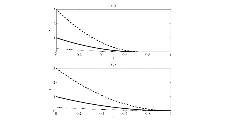
Figure 1: The decay of $\tau(({\bf{1}}\otimes\mathcal{E})|\psi\rangle\langle\psi|)$(solid line) and its upper(dashed line) and lower bound(dotted line), where (a):$\mathcal{E}$ is a depolarizing channel and (b):$\mathcal{E}$ is a phase damping channel. Here we let $d=3$, $\omega_{0}=\omega_{1}=\frac{1}{6}$ and $\omega_{2}=\frac{2}{3}$. Note that in (a) a sudden death of $\tau$ appears but in (b) it doesn’t.

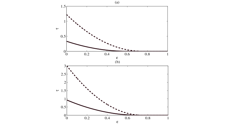
Figure 2: The decay of $\tau(({\bf{1}}\otimes\mathcal{E})\rho_{F})$(solid line) and its upper bound(dashed line), where $\mathcal{E}$ is a depolarizing channel and $d=3$. (a): $F=\frac{2}{3}$; (b): $F=\frac{8}{9}$. Note that $\tau$ and its upper bound both vanish in finite time, although maybe not at the same time.

Just like the sudden death of entanglement cannot appear for any channel [9], the sudden death of $\tau$ doesn’t exist for some channels. For example, for phase damping channel, we can see only when $\varepsilon=1$, $\tau(({\bf{1}}\otimes\mathcal{E})|\psi\rangle\langle\psi|)$ vanishes, which means $\tau$ doesn’t die suddenly but asymptotically. But, if the input state is mixed, for example a $3\otimes 3$ Werner state, the sudden death of $\tau$ can also appear even for phase damping channel.

Summary.— The dynamics of a system is a fundamental feature to describe its time evolution property. In this paper, we have shown the dynamical properties of the lower and upper bounds of squared concurrence respectively. Unlike the concurrence itself, the lower bound of the squared concurrence in this paper is computable. Thus our results are more reachable in various situations. We use depolarizing and phase damping channels as examples and find $\tau$ will vanish in finite time. Whether the entanglement sudden death appear depends both on the channel and the input state. Our result provides an easy way to estimate the dynamics of the entanglement in realistic physical systems.

Acknowledgements: HF acknowledges the support by ”Bairen” program, NSFC grant (10674162) and ”973” program (2006CB921107).