Eigenvalue problem in two dimension for an irregular boundary

Abstract

An analytical perturbative method is suggested for determining the eigenvalues of the Helmholtz equation $(\nabla^{2}+k^{2})\psi=0$ in two dimensions where $\psi$ vanishes on an irregular closed curve. We can thus find the energy levels of a quantum mechanical particle confined in an infinitely deep potential well in two dimensions having an irregular boundary or the vibration frequencies of a membrane whose edge is an irregular closed curve. The method is tested by calculating the energy levels for an elliptical and a supercircular boundary and comparing with the results obtained numerically. Further, the phenomenon of level crossing due to shape variation is also discussed.

I Introduction

The energy levels of a quantum particle confined in a 2D regular box can be solved exactly only in the cases of a square and a triangle and in the limiting case of a circle. While the determination of the energy levels for the circular or the square boundary is a trivial exercise, the problem of the triangular boundary is more formidable Krishnamurthy . The corresponding problems in the classical regime can be the flow of liquid through a pipe of polygonal cross-section or the free vibration of a membrane (with a fixed boundary) of polygonal shape. The classical problems, like their quantum counterparts, are amenable to simple analytical treatments only in the cases of a circle, a square and a triangle. The problem of a regular polygonal box has been solved by perturbing about the equivalent circle and the results have been quite accurate Jayanta . The same problem has been solved by Cureton and Kuttler Cureton in the context of vibration of membranes. Here we address the problem of finding out the energy eigenvalues when the boundary has no simple geometric shape. The Schrödinger equation for a particle of mass $m$ and energy $E$ confined in an infinitely deep 2D potential well is,

$$-{{\hbar^{2}}\over{2m}}\nabla^{2}\psi=E\psi.$$ (1a)

The above equation can be recast as,

$$(\nabla^{2}+k^{2})\psi=0,$$ (1b)

where $k=\sqrt{\frac{2mE}{\hbar^{2}}}$. Thus the problem boils down to solving the Helmholtz equation with the Dirichlet condition $\psi=0$ on the ‘irregular’ boundary. Exact solutions can be obtained only in a few special cases as mentioned earlier. The standard procedure is to choose a curvilinear coordinate system suited to the geometry of the problem and employ the method of separation of variables. For a boundary having an irregular shape no particular coordinate system will be useful. Hence, we resort to perturbative methods to solve the problem. Here we will perturb the boundary about a circle so that in our problem solutions can be obtained in the form of corrections to the solutions for the circular boundary. Till now, most of the efforts at finding out the eigenvalues of the Helmholtz equation for an irregular boundary have been numerical. Mazumdar M1 ; M2 ; M3 reviews the approximate methods invoked for this problem. In addition to the extensive summary of theoretical results, Kuttler and Sigillito Kuttler also give a comprehensive review of the different numerical methods employed. More recently, Amore Amore gives a numerical recipe using a collocation approach based on little sinc functions. As far as analytical works are concerned, Rayleigh Rayleigh and also Fetter and Walecka Fetter find the ground state energy eigenvalues for a vibrating membrane. A general formalism has been suggested by Morse and Feshbach Morse using the Green functions. Parker and Mote Parker have put forward a perturbative method for finding the eigenvalues and the eigenfunctions through fifth order. A similar method has been proposed by Nayfeh Nayfeh . However, the eigenvalues are found out only to the first order. Read Read has also suggested a general analytical approach to the problem. Bera et al Bera have proposed a perturbative approach to the problem but failed to express the solutions in a closed form. Our approach is similar in spirit to that of Bera. Here we present a solution to the problem in a more systematic and efficient manner. The perturbative correction to the eigenvalues and the eigenfunctions are presented in a closed form at each order of perturbation. The method is tested by comparing the analytical results with those obtained numerically for a supercircular and an elliptical boundary. Further, the phenomenon of energy level crossing as induced by the shape variation is also dealt with for both the boundaries. In section II we set up our general scheme and in section III we apply it to the cases of a supercircle and an ellipse. A short conclusion is presented in section IV.

II Perturbation about the Equivalent Circle

It was shown by Rayleigh Rayleigh that the fundamental frequency of a membrane whose boundary is not extravagantly elongated is nearly same as that of a mechanically similar circular membrane having the same area. The above result naturally leads us to develop, in following, a perturbation about the equal area circle. Given, any $r(\theta)=r(\theta+2\pi)$, defining the boundary in 2D enclosing an area, $A={1\over 2}\int_{0}^{2\pi}r^{2}(\theta)d\theta$, we first construct a circle of radius, $R_{0}$, such that,

$$A=\pi R_{0}^{2}.$$ (2)

We can then expand $r(\theta)$ about $R_{0}$ in terms of Fourier series at different orders of smallness (denoted by $\lambda$) as,

$$r(\theta)=R_{0}\left[1+\sum_{\sigma=1}^{\infty}\lambda^{\sigma}f^{(\sigma)}(\theta)\right],$$ (3)

where,

$$f^{(\sigma)}(\theta)=\sum_{n=0}^{\infty}(C_{n}^{(\sigma)}\cos n\theta+S_{n}^{(\sigma)}\sin n\theta).$$ (4)

Here, for simplicity, we have considered a one parameter (deformation parameter), $\lambda$, dependence of $r(\theta)$, which thus represents a family of curves which reduce to the equation for a circle in the limiting case $\lambda\to 0$. In principle, $\lambda$ should be much smaller than unity ensuring that the variation of $r(\theta)$ with $\theta$ is small enough to permit the use of perturbative methods. However, as we will see in the next section that for the case of a supercircle $\lambda\sim 1$ works quite well and keeps the results within 10% error. We also note here that the Fourier expansion of the boundary in (3) is rather unusual and which makes our method different from all other existing methods. Here in fact each $f^{(\sigma)}(\theta)$ is a Fourier series in itself of order $\lambda^{\sigma}$. Earlier methods in the literature had worked with only one Fourier series - that is by summing all the orders into one. The main advantage in treating the problem like this is to have an analogy with the time independent perturbation scheme of quantum mechanics and obtain closed form solutions at each order of $\lambda$. If we now calculate the area using (3), (4) and equate it with $\pi R_{0}^{2}$, we arrive at the following constraint relations among the Fourier coefficients,

$$\sum_{n=0}^{\infty}\sum_{\nu=1}^{\sigma-1}\left[C_{n}^{(\nu)}C_{n}^{(\sigma-\nu)}+2C_{0}^{(\nu)}C_{0}^{(\sigma-\nu)}+S_{n}^{(\nu)}S_{n}^{(\sigma-\nu)}\right]=-4C_{0}^{(\sigma)}.$$ (5a)

In particular we have,

$$C_{0}^{(1)}=0,$$ (5b)

and

$$4C_{0}^{(2)}=-\sum_{n=1}^{\infty}[C_{n}^{(1)2}+S_{n}^{(1)2}].$$ (5c)

Now, as a first approximation, the energy $E_{0}$ of the particle confined by $r(\theta)$ will be that of a particle enclosed in a circle of radius $R_{0}$,

$$E_{0}=\frac{\hbar^{2}\rho_{l,j}^{2}}{2mR_{0}^{2}},$$ (6)

with $\rho_{l,j}=k_{l,j}R_{0}$ being the $j^{\rm th}$ node of the $l^{\rm th}$ order Bessel function. The next step is to improve upon the ‘equal area’ approximation by perturbing the equivalent circle and finding out the first and the second order corrections to the eigenvalues.
We now treat $\lambda$ as the perturbation parameter and expand $\psi$ and $E$ as,

$$\psi=\psi_{0}+\lambda\psi_{1}+\lambda^{2}\psi_{2}+...,$$ (7a)

$$E=E_{0}+\lambda E_{1}+\lambda^{2}E_{2}+...~{}.$$ (7b)

Using (7a), (7b) in (1a), equating the coefficients of different powers of $\lambda$ to 0 and after some rearrangement we arrive at the set of equations,

$$(\nabla^{2}+\frac{2mE_{0}}{\hbar^{2}})\psi_{0}=0,$$ (8a)

$$(\nabla^{2}+\frac{2mE_{0}}{\hbar^{2}})\psi_{1}=-\frac{2mE_{1}}{\hbar^{2}}\psi_{0},$$ (8b)

$$(\nabla^{2}+\frac{2mE_{0}}{\hbar^{2}})\psi_{2}=-\frac{2m}{\hbar^{2}}({E_{1}}{\psi_{1}}+{E_{2}}{\psi_{0}}).$$ (8c)

Equation (8a) can readily be identified as the equation for the circular boundary with $\psi_{0}$ as the eigenfunction corresponding to energy $E_{0}$.
The boundary condition is,

$$\psi(R_{0}+\lambda R_{0}f^{(1)}+\lambda^{2}R_{0}f^{(2)}+...)=0.$$

Taylor expanding about $r=R_{0}$, with (7a) and equating the coefficients of different powers of $\lambda$ to 0, we find,

$$\psi_{0}(R_{0})=0,$$ (9a)

$$\psi_{1}(R_{0})+R_{0}f^{(1)}\psi_{0}^{{}^{\prime}}(R_{0})=0,$$ (9b)

$$\psi_{2}(R_{0})+R_{0}f^{(1)}\psi_{1}^{{}^{\prime}}(R_{0})+R_{0}f^{(2)}\psi_{0}^{{}^{\prime}}(R_{0})+\frac{1}{2}R_{0}^{2}f^{(1)2}\psi_{0}^{{}^{\prime\prime}}({R_{0}})=0.$$ (9c)

We discuss separately the cases $l=0$ and $l\neq 0$.

II.1 Calculation of Energy for $l=0$ State

For the $l=0$ state,

$$\psi_{0}=NJ_{0}(\rho),$$ (10)

where $\rho=kr$, $J_{0}$ is the $0^{\rm th}$ order Bessel function, and $N=1/({\sqrt{\pi}R_{0}J_{1}(\rho_{0,j})})$, is the normalisation constant. $E_{0}$ is obtained from (6) with $l=0$, and an appropriate $j$, as $\psi_{0}$ satisfies boundary condition (9a). The first order correction to the wave function, obtained as a solution to (8b) is,

$$\psi_{1}=\sum_{p=1}^{\infty}(a_{p}\cos p\theta+\bar{a}_{p}\sin p\theta)J_{p}+a_{0}J_{0}-\frac{\rho E_{1}}{2E_{0}}NJ_{1},$$ (11)

where the last term is the particular integral to (8b). Incorporating (11) in (9b) and separately matching the coefficients of the cosine and the sine terms we have,

$$a_{p}=-\rho_{0,j}NC_{p}^{(1)}\frac{J_{0}^{\prime}(\rho_{0,j})}{J_{p}(\rho_{0,j})},$$ (12a)

$$\bar{a}_{p}=-\rho_{0,j}NS_{p}^{(1)}\frac{J_{0}^{\prime}(\rho_{0,j})}{J_{p}(\rho_{0,j})},$$ (12b)

$$E_{1}=0.$$ (12c)

The remaining constant $a_{0}$ can be found out by normalising the corrected wave function over the enclosed area. However, that is not required right now for our purpose. (12c) implies that there cannot be any correction to the energy in the first order. So any possible correction to the energy can only come from the second or higher orders. In a similar fashion the second correction to the wave function as a solution to (8c) with $E_{1}=0$ is found out to be,

$$\psi_{2}=\sum_{p=1}^{\infty}(b_{p}\cos p\theta+\bar{b}_{p}\sin p\theta)J_{p}+b_{0}J_{0}-\frac{\rho E_{2}}{2E_{0}}NJ_{1},$$ (13)

which, when introduced in (9c), now yields,

$$E_{2}=E_{0}\left[\sum_{k=1}^{\infty}(C_{k}^{(1)2}+S_{k}^{(1)2})\left[\frac{1}{2}+\rho_{0,j}\frac{J_{k}^{\prime}(\rho_{0,j})}{J_{k}(\rho_{0,j})}\right]-2C_{0}^{(2)}\right],$$ (14a)

$$b_{p}=-\rho_{0,j}\frac{J_{0}^{\prime}(\rho_{0,j})}{J_{0}(\rho_{0,j})}\left[NC^{(2)}_{p}+a_{0}C_{p}^{(1)}\right]$$

$$+\frac{\rho_{0,j}J_{0}^{\prime}(\rho_{0,j})N}{2J_{0}(\rho_{0,j})}\sum_{k=1}^{\infty}[C_{p+k}^{(1)}C_{k}^{(1)}+S_{p+k}^{(1)}S_{k}^{(1)}+C_{|p-k|}^{(1)}C_{k}^{(1)}$$

$$-S_{p-k}^{(1)}S_{k}^{(1)}+S_{k-p}^{(1)}S_{k}^{(1)}]\left(\frac{1}{2}+\rho_{0,j}\frac{J_{k}^{\prime}(\rho_{0,j})}{J_{k}(\rho_{0,j})}\right),$$ (14b)

$$\bar{b}_{p}=-\rho_{0,j}\frac{J_{0}^{\prime}(\rho_{0,j})}{J_{0}(\rho_{0,j})}\left[NS_{p}^{(2)}+a_{0}S_{p}^{(1)}\right]$$

$$+\frac{\rho_{0,j}J_{0}^{\prime}(\rho_{0,j})N}{2J_{0}(\rho_{0,j})}\sum_{k=1}^{\infty}[S_{p+k}^{(1)}C_{k}^{(1)}-C_{p+k}^{(1)}S_{k}^{(1)}+C_{|p-k|}^{(1)}S_{k}^{(1)}$$

$$-S_{k-p}^{(1)}C_{k}^{(1)}+S_{p-k}^{(1)}C_{k}^{(1)}]\left(\frac{1}{2}+\rho_{0,j}\frac{J_{k}^{\prime}(\rho_{0,j})}{J_{k}(\rho_{0,j})}\right).$$ (14c)

As before, the remaining constant $b_{0}$ can be determined by normalising the wave function up to the order of $\lambda^{2}$.

II.2 Calculation of Energy for $l\neq 0$ state

The $l\neq 0$ states come in 2 varieties,

$$\psi_{0}=N_{l}J_{l}(\rho)\left(\begin{array}[]{c}\cos l\theta\\ \sin l\theta\end{array}\right),$$ (15)

where, $N_{l}=\sqrt{2}/({\sqrt{\pi}R_{0}J^{\prime}_{l}(\rho_{l,j})})$. $E_{0}$ is given by (6). For simplicity, we assume that $S_{n}^{(\sigma)}=0$ for all $\sigma$. We shall first work with

$$\psi_{0}=N_{l}J_{l}(\rho)\cos l\theta.$$ (16)

The result for the other case will be similar. The first correction to the wave function obtained as a solution to (8b) is,

$$\psi_{1}=\sum_{p=0,p\neq l}^{\infty}a_{p}J_{p}\cos p\theta+\left(a_{l}J_{l}-\frac{E_{1}}{E_{0}}\frac{\rho}{2}N_{l}J_{l+1}\right)\cos l\theta.$$ (17)

Following a similar procedure as that for the ground state we now have,

$$E_{1}=-C_{2l}^{(1)}E_{0},$$ (18a)

$$a_{p}=-\frac{\rho_{l,j}}{2}N_{l}\frac{J_{l}^{\prime}(\rho_{l,j})}{J_{p}(\rho_{l,j})}(C_{p+l}^{(1)}+C_{|p-l|}^{(1)}),~{}~{}~{}~{}\text{for $p\neq 0,l$},$$ (18b)

$$a_{0}=-\frac{\rho_{l,j}}{2}N_{l}\frac{J_{l}^{\prime}(\rho_{l,j})}{J_{0}(\rho_{l,j})}C_{l}^{(1)}.$$ (18c)

$a_{l}$ can be obtained from the normalisation condition. The second order corrections yield,

$$\psi_{2}=\sum_{m=0}^{\infty}\left[b_{m}J_{m}-\frac{\rho E_{1}}{2E_{0}}a_{m}J_{m+1}\right]\cos m\theta+\left[C_{2l}^{(1)2}\frac{\rho}{4}J_{l+2}-\frac{E_{2}}{E_{0}}J_{l+1}\right]N_{l}\frac{\rho}{2}\cos l\theta,$$ (19a)

$$\frac{E_{2}}{E_{0}}=\frac{C_{2l}^{(1)2}}{2}+\frac{1}{4}\sum_{n=1}^{\infty}C_{n}^{(1)}(2C_{n}^{(1)}+C_{2l+n}^{(1)}+C_{|2l-n|}^{(1)})-2C_{0}^{(2)}$$

$$-C_{2l}^{(2)}+\sum_{{n=1}\atop{n\neq l}}^{\infty}(C_{n+l}^{(1)}+C_{|n-l|}^{(1)})^{2}\frac{\rho_{l,j}J_{n}^{\prime}(\rho_{l,j})}{2J_{n}(\rho_{l,j})}+C_{l}^{(1)2}\frac{\rho_{l,j}J_{0}^{\prime}(\rho_{l,j})}{J_{0}(\rho_{l,j})}.$$ (19b)

The constants $b_{m}$ can also be determined as in the case of the ground state. However, they are not needed for now. Need for them would arise when one would evaluate the third order correction for energy. For the case,

$$\psi_{0}=N_{l}J_{l}(\rho)\sin l\theta,$$ (20)

similar calculations result in,

$$\psi_{1}=\sum_{p=1,p\neq l}^{\infty}\bar{a}_{p}J_{p}\sin p\theta+\left(\bar{a}_{l}J_{l}-\frac{E_{1}}{E_{0}}\frac{\rho}{2}N_{l}J_{l+1}\right)\sin l\theta,$$ (21a)

$$E_{1}=C_{2l}^{(1)}E_{0},$$ (21b)

$$\bar{a}_{p}=\frac{\rho_{l,j}}{2}N_{l}\frac{J_{l}^{\prime}(\rho_{l,j})}{J_{p}(\rho_{l,j})}(C_{p+l}^{(1)}-C_{|p-l|}^{(1)}),~{}~{}~{}~{}\text{for $p\neq l$},$$ (21c)

$$\psi_{2}=\sum_{m=1}^{\infty}\left[\bar{b}_{m}J_{m}-\frac{\rho E_{1}}{2E_{0}}\bar{a}_{m}J_{m+1}\right]\sin m\theta+\left[C_{2l}^{(1)2}\frac{\rho}{4}J_{l+2}-\frac{E_{2}}{E_{0}}J_{l+1}\right]N_{l}\frac{\rho}{2}\sin l\theta,$$ (21d)

and

$$\frac{E_{2}}{E_{0}}=\frac{C_{2l}^{(1)2}}{2}+\frac{1}{4}\sum_{n=1}^{\infty}C_{n}^{(1)}(2C_{n}^{(1)}-C_{2l+n}^{(1)}-C_{|2l-n|}^{(1)})-2C_{0}^{(2)}$$

$$+C_{2l}^{(2)}+\sum_{n=1,n\neq l}^{\infty}\left(C_{n+l}^{(1)}-C_{|n-l|}^{(1)}\right)^{2}\frac{\rho_{l,j}J_{n}^{\prime}(\rho_{l,j})}{2J_{n}(\rho_{l,j})}.$$ (21e)

We do not give the expressions for $\bar{b}_{m}$, as they are not needed now.

III Application to Simple Cases

The general formalism having been outlined above we now estimate the energy levels of a supercircle and an ellipse where direct comparison with the numerical results can be made. Numerical results were calculated using the finite difference method. Both square and triangular grids were used separately for the numerical simulation. The results agree quite well for both types of grids.

III.1 Particle Enclosed in a Supercircular Enclosure

Piet Hein Superellipse Gardner is a special case of Lamé curves described by,

$$\frac{|x|^{t}}{a^{t}}+\frac{|y|^{t}}{b^{t}}=1,$$ (22)

with $t>1$. $a$ and $b$ are positive real numbers. They are also known as Lamé curves or Lamé ovals Gridgeman . Superellipses can be parametrically described as,

$$x=a\cos^{{2}/{t}}\phi,~{}~{}{\rm and}~{}~{}y=b\sin^{{2}/{t}}\phi.$$ (23)

Different values of $t$ would give us closed curves of different shapes. For $t>1$ we consider only the real positive values of $\cos^{{2}/{t}}\phi$ and $\sin^{{2}/{t}}\phi$ for $0\leqslant\phi\leqslant\frac{\pi}{2}$ and use the symmetry of the figure to continue to the other quadrants. We are interested in the case $a=b$, which corresponds to a supercircle. In polar coordinates the equation for the supercircle is,

$$r=\frac{a}{(\cos^{t}\theta+\sin^{t}\theta)^{\frac{1}{t}}},$$ (24)

and the radius of the equal area circle is,

$$R_{0}=a\sqrt{\frac{2}{t\pi}}\frac{[\Gamma(\frac{1}{t})]}{\sqrt{[\Gamma(\frac{2}{t})]}}.$$ (25)

Figure 1: Shape of the supercircle for different values of $t$

.

The shapes of supercircles for different values of $t$ are shown in FIG.1. $t=2$ describes a circle of unit radius. In this case we have a natural deformation parameter, $\lambda=2-t$. Now $r(\theta)$, given by (24) can be Fourier expanded and after some calculation one arrives at the following,

$$r(\theta)=R_{0}[1+\lambda\sum_{n=1}^{\infty}C_{4n}^{(1)}\cos 4n\theta+\lambda^{2}\sum_{n=0}^{\infty}C_{4n}^{(2)}\cos 4n\theta+{\rm O}(\lambda^{3})...],$$ (26)

where the Fourier coefficients are found to be,

$$C_{4n}^{(1)}=-\frac{1}{4n(4n^{2}-1)},$$

$$C_{0}^{(2)}=-\frac{1}{4}\sum_{n=1}^{\infty}\left[\frac{1}{4n(4n^{2}-1)}\right]^{2}$$

$$\phantom{aaaa\qquad}={\frac{1}{16}}\left(1-{\frac{5\pi^{2}}{48}}\right)=-0.0017552,$$

using (5c) and

$$C_{4}^{(2)}=\frac{1}{32}\left(\frac{3\pi^{2}}{8}-\frac{23}{9}\right)=0.0357983.$$

Using these Fourier coefficients, the first six energy levels are calculated for the supercircular boundary in the range $-1\leqslant\lambda\leqslant 1$, and compared with the numerically obtained values. This is shown in FIG.2.

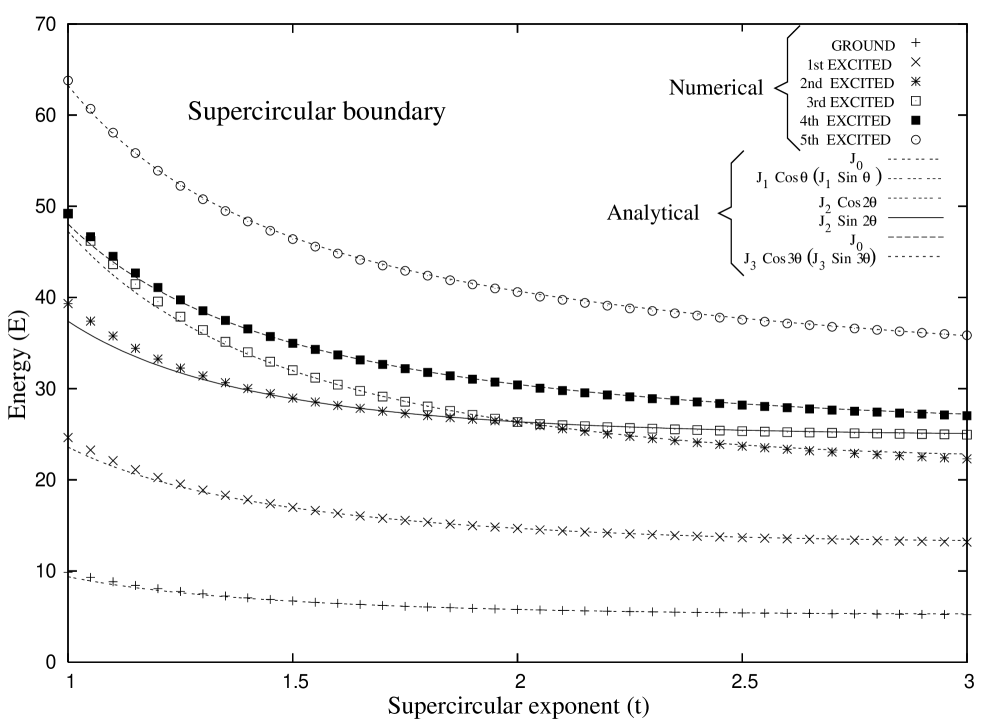
Figure 2: Comparison of the energy eigenvalues obtained numerically and analytically for a particle enclosed in a supercircular boundary shown for the first 6 states (in units of $\frac{\hbar^{2}}{2mR_{o}^{2}}$). Deformation parameter $\lambda=2-t$.

The numerical results are shown by discrete points and the analytical ones by the continuous lines. The fact that even for such a wide range of $\lambda$ the analytical results are in fairly good agreement with those obtained numerically does indeed justify the validity of our formalism. We see that for $|\lambda|$ as large as 1 the deviations of analytical values from the numerical ones are within 10%. Furthermore, it is to be noted that the energy level corresponding to the unperturbed wave function $\psi_{0}=N_{2}J_{2}\cos 2\theta$ is strongly affected compared to the others and crosses over to its counterpart $\psi_{0}=N_{2}J_{2}\sin 2\theta$ at $\lambda=0$. This crossing of energy levels is solely induced by the variation in the shape of the boundary of the potential well.

III.2 Particle Enclosed in an Elliptical Enclosure

The determination of the eigenvalues of the Helmholtz operator in 2D with an elliptical boundary has been investigated extensively. In this case the variable separation is possible in elliptical coordinate system and the problem is exactly solvable in principle. The problem reduces to solving the Mathieu differential equation for each of the separated coordinates. Extracting out the eigenvalues and the eigenfuctions from the above is a difficult task and often one relies on numerical estimation. So far most of the efforts have been directed at the numerical estimation of the eigenvalues Wilson ; Hettich ; Troesch . Recently, an analytical method has been suggested by Wu and Shivakumar Yan . Here we propose a simpler approach to the problem by our perturbative method. The equation for an ellipse with semi-axes $a$ and $b$, in polar coordinates is,

$$r(\theta)=\frac{b}{\sqrt{1-(1-\frac{b^{2}}{a^{2}})\cos^{2}\theta}},$$ (27)

Defining the deformation parameter,

$$\lambda=\frac{a-b}{a+b},$$ (28)

we show the shapes of the ellipses for different values of $\lambda$ in FIG.3.

Figure 3: Shape of the ellipse for different values of $\lambda=\frac{a-b}{a+b}.$

Again $\lambda=0$ describes a circle with unit radius. Now, $r(\theta)$ in (27) can be recast as,

$$r=R_{0}[1+\lambda\cos 2\theta-\frac{1}{4}\lambda^{2}+\frac{3}{4}\lambda^{2}\cos 4\theta+{\rm O}(\lambda^{3})+...],$$ (29)

with $R_{0}=\sqrt{ab}$. Comparing with our general Fourier series of (4), we observe that,

$$C_{2}^{(1)}=1,~{}~{}C_{0}^{(2)}=-\frac{1}{4},~{}~{}{\rm and}~{}~{}C_{4}^{(2)}=\frac{3}{4}.$$

Using (12c),(14a),(18a),(19b), (21b),(21e) we find,

$$E_{1}\left(\begin{array}[]{c}J_{l}\cos l\theta\\ J_{l}\sin l\theta\end{array}\right)=\left(\begin{array}[]{c}-\\ +\end{array}\right)E_{0}\delta_{l1},$$ (30a)

and

$$E_{2}\left(\begin{array}[]{c}J_{l}\cos l\theta\\ J_{l}\sin l\theta\end{array}\right)=E_{0}\left(\frac{\delta_{l1}}{2}+1+\sum_{p,|p-l|=2}\frac{\rho_{l,j}J_{p}^{\prime}(\rho_{l,j})}{2J_{p}(\rho_{l,j})}\right)$$

$$+\left(\begin{array}[]{c}-\frac{3}{4}+\frac{\rho_{l,j}J_{0}^{\prime}(\rho_{l,j})}{J_{0}(\rho_{l,j})}\\ \frac{3}{4}\end{array}\right)E_{0}\delta_{2l},$$ (30b)

where $\delta_{ij}$ is Kronecker delta. The results for the elliptical boundary are shown in FIG.4.

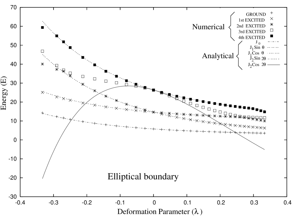
Figure 4: Comparison of the energy eigenvalues obtained numerically and analytically for a particle confined in an elliptical boundary shown for the first 5 states (in units of $\frac{\hbar^{2}}{2mR_{o}^{2}}$). Deformation parameter $\lambda=\frac{a-b}{a+b}.$

From FIG.4 it is seen that as in the case of the supercircle here also the $J_{1}\cos\theta$ state is strongly affected by the boundary perturbation and crosses over to its counterpart $J_{1}\sin\theta$ at $\lambda=0$. However, quite interestingly, the $J_{2}$ states do not cross but are rather repelled by each other. They touch each other tangentially at $\lambda=0$. While for one of these states, $J_{2}\sin 2\theta$ the analytical method works quite well, it has a restricted validity for the other one, viz. $J_{2}\cos 2\theta$. In fact, we compared the energy levels for the first 10 states and found out the agreement between the analytical and the numerical results to be quite satisfactory except when the levels repel each other. This phenomenon of level repulsion also goes by the name of “loci veering” in the literature. In case of level repulsion the validity of the perturbation theory for the $J_{l}\cos l\theta$ states is restricted to a small range in $\lambda$ (e.g. $|\lambda|\leqq 0.08$). This is in sharp contrast to the case where there is no repulsion in which case the agreement with the perturbation theory persists over a wide range.

IV Conclusion

One of the principle virtues of the method proposed is its generality. With slight modification, the formalism can readily be adopted to study the shape dependence of the eigenvalues of a vibrating membrane with Dirichlet conditions on an irregular boundary. The approach can also be useful in studying the modes of propagation of electromagnetic waves in a waveguide with irregular cross section. In fact, recently, Dubertrand et al Dubertrand have employed a similar scheme for the propagation of electromagnetic waves in open dielectric systems. Another potential area where this formalism might be useful is in the study of quantum dots. This field has been an area of vigorous research for the past few years. 2D quantum dots are generally taken to have a circular symmetry. However, in practice such a symmetry can not be strictly ensured. There is bound to be small deviations from exact circular symmetry. Hence, probes have been constructed to investigate the shape of the dots Lis ; Drouvelis ; Prb . As shown in this paper the energy eigenvalues of a particle confined in 2D in an infinitely deep potential well will essentially depend upon the shape of the confining region. Hence a study of the shape dependence of the energy levels might prove to be useful in shedding light upon the actual shapes of the dots. Another significant aspect of our formalism is the use of the general Fourier series to express the deviation of the boundary from a circular one which allows us to treat any sort of boundary within the limit of small perturbation for which our formalism is valid. Even boundaries with sharp singularities can be treated in our formalism quite efficiently. For example, the square which is a special case of a supercircle with $t=1$ can be treated quite efficiently by our method. This is borne out by the accuracy of the results obtained by using our formalism in the case of the supercircle for $t=1~{}(\lambda=1)$, which corresponds to a square [FIG.1 and FIG.2]. In fact, to find out the energy and the wave function corrections all one needs is to find the Fourier coefficients for the closed curve and substitute them in the relevant expressions. Further, the corrections to the energy eigenvalue and the eigenfunctions are found out exactly in a closed form at each order of perturbation without any major approximations which is indeed remarkable. The case of the supercircular boundary shows that even for quite large perturbations the method yields satisfactory results. The accuracy of the method can be still improved by including higher order corrections. In fact, we have also found out the third order corrections, although the results are not included here. On the contrary, the case of the elliptical boundary points out to the failure of the perturbation theory whenever the energy levels exhibit repulsion. This provides potential topics for future investigations. Another point which we want to emphasis here is that the success (and also the efficiency) of the formalism depends to a large extent upon the judicious choice of the deformation parameter $\lambda$. For the case of the ellipse we defined $\lambda$ to be equal to $\frac{a-b}{a+b}$ whereas the eccentricity $\epsilon$ would seem to be a more appropriate candidate for $\lambda$. For the elliptical boundary we have considered deformations up to the extent where $a:b=2:1$ for which $\lambda=0.333$. Had we formulated the problem in terms of the eccentricity the same deformation would have led to the value of $\epsilon=0.866$. It can also be shown that in that case the deformation parameter would actually be $\epsilon^{2}$, so that for the same deformation we would have $\epsilon^{2}=0.75$ which is obviously much larger than the parameter which we have actually used here. Such a high value of the deformation parameter goes against the very essence of the perturbative nature of the method. This means that while we have terminated the Fourier series and also the eigenvalues at the second order of smallness when working with $\lambda=\frac{a-b}{a+b}$, for $\lambda=\epsilon^{2}$ we would have to consider higher order terms to get the same accuracy. Finally, we note that the same formalism can also be adopted by perturbing a square or a rectangular boundary for which the results are exactly known.

- (1) Krishnamurthy H R, Mani H S, Verma H C 1982 J. Phys. A: Math. Gen., 15(2131)
- (2) Bhattacharjee J K, Banerjee K 1987 J. Phys. A: Math. Gen., 20 (L759)
- (3) Cureton L M, Kuttler J R 1999 Journal of Sound and Vibration, 220(1) (83)
- (4) Mazumdar J 1975 Shock and Vibration Digest, 7 (75)
- (5) Mazumdar J 1979 Shock and Vibration Digest, 11 (25)
- (6) Mazumdar J 1982 Shock and Vibration Digest, 14 (11)
- (7) Kuttler J R, Sigillito V G 1984 SIAM Review, 26 (163)
- (8) Amore P 2008 J. Phys. A : Math. Theor., 41 (265206)
- (9) Rayleigh J W S B Theory of Sound, 2nd. ed., Dover, New York (1945)
- (10) Fetter A L, Walecka J D Theoretical Mechanics of Particles and Continua, McGraw Hill Book Company (1980)
- (11) Morse P M, Feshbach H Methods of Theoretical Physics, Vol.2, McGraw Hill Book Company (1983)
- (12) Parker R G, Mote C D Jr. Journal of Sound and Vibration, 1998 211(3) (389)
- (13) Nayfeh A H Introduction to Perturbation Techniques, J. Wiley, New York (1981)
- (14) Read W W 1996 Mathematical and Computer Modelling, 24 No.2 (23)
- (15) Bera N, Bhattacharjee J K, Mitra S, Khastgir S P 2008 Eur. Phys. J. D,46 (41)
- (16) Gardner M, “Piet Hein’s Superellipse”, Ch. 18 in Mathematical Carnival: A new Round-Up of Tantalizers and Puzzles from Scientific American., New York: Vintage, pp. 240-254, (1977)
- (17) Gridgeman N T, “Lamé Ovals.” Math. Gaz. 1970 54, (31-37)
- (18) Wilson H B, Scharstein R W 2007 Journal of Engineering Mathematics, 57 1 (41)
- (19) Hettich R, Haaren E, Ries M, Still G 1987Journal of Applied Mathematics and Mechanics, 67 12 (589)
- (20) Troesch B A, Troesch H R 1973 Mathematics of Computation, 27 24
- (21) Wu Yan, Shivakumar P N 2008 Computers and Mathematics with Applications, 55 6 (1129)
- (22) Dubertrand R, Bogomolny E, Djellali N, Lebental M, Schmit C 2008 Physical Review A 77 (013804)
- (23) Lis K, Bednarek S, Szafran B, Adamowski J 2003 Physica E 17 ( 494 )
- (24) Drouvelis P S, Schmelcher P, Diakonos F K 2004 Physical Review B 69 ( 155312 )
- (25) Magnúsdóttir I, Gudmundsson V 1999 Physical Review B 60 ( 16590 )