An XMM-Newton Spectral and Timing Study of IGR J16207–5129: An Obscured and Non-Pulsating HMXB

Abstract

We report on a $\sim$12 hr XMM-Newton observation of the supergiant High-Mass X-ray Binary IGR J16207–5129. This is only the second soft X-ray (0.4–15 keV, in this case) study of the source since it was discovered by the INTEGRAL satellite. The average energy spectrum is very similar to those of neutron star HMXBs, being dominated by a highly absorbed power-law component with a photon index of $\Gamma=1.15^{+0.07}_{-0.05}$. The spectrum also exhibits a soft excess below $\sim$2 keV and an iron K$\alpha$ emission line at $6.39\pm 0.03$ keV. For the primary power-law component, the column density is $(1.19^{+0.06}_{-0.05})\times 10^{23}$ cm^-2, indicating local absorption, likely from the stellar wind, and placing IGR J16207–5129 in the category of obscured IGR HMXBs. The source exhibits a very high level of variability with an rms noise level of 64%$\pm$21% in the $10^{-4}$ to 0.05 Hz frequency range. Although the energy spectrum suggests that the system may harbor a neutron star, no pulsations are detected with a 90% confidence upper limit of $\sim$2% in a frequency range from $\sim$$10^{-4}$ to 88 Hz. We discuss similarities between IGR J16207–5129 and other apparently non-pulsating HMXBs, including other IGR HMXBs as well as 4U 2206+54 and 4U 1700–377.

1. Introduction

The hard X-ray imaging by the INTEGRAL satellite (Winkler et al., 2003) has been uncovering a large number of hard X-ray sources. Since INTEGRAL’s launch in 2002 October, 550 sources have been detected by the IBIS instrument in the $\sim$20–50 keV band (based on version 29 of the “General Reference Catalog”). Included in these sources are 236 “IGR” sources that were unknown or at least not well-studied prior to INTEGRAL. An important result from the INTEGRAL mission has been the discovery of a relatively large number of High-Mass X-ray Binaries (HMXBs). There are 37 IGR sources that have been classified as HMXBs (and it should be noted that about 1/3 of the IGR sources are still unclassified). The IGR HMXBs are interesting both for the large number of new systems as well as the specific properties of these systems. These include a new class of “Supergiant Fast X-ray Transients” (Negueruela et al., 2006) that are HMXBs that can exhibit hard X-ray flares that only last for a few hours while the X-ray flux changes by orders of magnitude (in ’t Zand, 2005; Sguera et al., 2006). Many of the IGR HMXBs are also extreme in having a high level of obscuration ($N_{\rm H}$$\sim$$10^{23}$–$10^{24}$ cm^-2) due to material local to the source (Walter et al., 2006; Chaty et al., 2008). For both the SFXTs and the obscured HMXBs, it is thought that a strong stellar wind is at least partially responsible for their extreme X-ray properties (Filliatre & Chaty, 2004; Walter et al., 2006; Walter & Zurita Heras, 2007).

The 37 IGR HMXBs presumably contain either neutron stars or black holes, but the nature of the compact object is only clear for the 12 systems for which X-ray pulsations from their neutron stars have been detected. Eleven of these systems have pulse periods ranging from 5 to 1300 s, and the 12th system has an unusually long period of $\sim$5900 s (Patel et al., 2004). Another X-ray property that can be taken as evidence for the presence of a neutron star is a very hard X-ray spectrum. Typically, neutron star HMXBs have X-ray spectra that can be modeled with a power-law with a photon index of $\Gamma$$\sim$1 that is exponentially cutoff near 10–20 keV (Nagase, 1989; Lutovinov et al., 2005). Although there are only a few known black hole HMXBs (e.g., Cygnus X-1, LMC X-1, LMC X-3, M33 X-7), their X-ray spectral properties are similar to the general class of black hole X-ray binaries with power-law spectra with $\Gamma$$\sim$1.4–2.1 in their hardest spectral state (McClintock & Remillard, 2006). If black hole spectra show a cutoff, it is usually close to 100 keV (Grove et al., 1998), significantly higher than seen for neutron star HMXBs. However, it should be noted that evidence from the shape of the spectral continuum alone is usually taken only as an indication of the nature of the compact object. For example, HMXBs 4U 1700–37 and 4U 2206+54 both have continuum X-ray spectra similar to neutron star HMXBs, but they are considered to be only probable neutron star systems because pulsations have not been detected.

In this study, we focus on X-ray observations of IGR J16207–5129, which was discovered in the Norma region of the Galaxy relatively early-on in the INTEGRAL mission (Walter et al., 2004; Tomsick et al., 2004). Although it is a relatively faint hard X-ray source at $3.3\pm 0.1$ millicrab in the 20–40 keV band (Bird et al., 2007), it has been consistently detected by INTEGRAL as well as in X-ray follow-up observations by Chandra and XMM-Newton (this work), indicating that it is a persistent source. The Chandra observation provided a sub-arcsecond position that allowed for the identification of an optical counterpart with $R=15.38\pm 0.03$ and an IR counterpart with $K_{\rm s}=9.13\pm 0.02$ (Tomsick et al., 2006). Based on the optical/IR Spectral Energy Distribution, Tomsick et al. (2006) found that the system has a massive O- or B-type optical companion. Optical and IR observations confirmed this and indicate a supergiant nature for the companion (Masetti et al., 2006; Negueruela & Schurch, 2007; Rahoui et al., 2008), and Rahoui et al. (2008) estimated a source distance of $\sim$4.1 kpc. With further IR spectroscopy, the spectral type of the companion was narrowed down to B1 Ia and a source distance of $6.1^{+8.9}_{-3.5}$ kpc was estimated (Nespoli, Fabregat & Mennickent, 2008).

Our current knowledge about the soft X-ray properties of IGR J16207–5129 comes from the Chandra observation that was made in 2005. This showed that the source has a hard X-ray spectrum with a power-law photon index of $\Gamma=0.5^{+0.6}_{-0.5}$, and the source also exhibited significant variability over the 5 ks Chandra observation (Tomsick et al., 2006). Based on these properties, we selected this target for follow-up XMM-Newton observations to obtain an improved X-ray spectrum and to search for pulsations that would provide information about the nature of the compact object. Here, we present the results of the XMM-Newton observation.

2. XMM-Newton Observations and Light Curve

We observed IGR J16207–5129 with XMM-Newton during satellite revolution 1329. The observation (ObsID 0402920201) started on 2007 March 13, 8.27 hr UT and lasted for 44 ks. The EPIC/pn instrument (Strüder et al., 2001) accumulated $\sim$0.4–15 keV photons in “small window” mode, giving a 4.4-by-4.4 arcminute² field-of-view (FOV) and a time resolution of 5.6718 ms. The mode used for the 2 EPIC/MOS units (Turner et al., 2001) is also called “small window” mode, and for MOS, its features are a 1.8-by-1.8 arcminute² FOV and a time resolution of 0.3 s. In addition to the XMM-Newton data, we downloaded the “current calibration files” indicated as necessary for this observation by the on-line software tool cifbuild. For further analysis of the data, we used the XMM-Newton Science Analysis Software (SAS-8.0.0) as well as the XSPEC package for spectral analysis and IDL for timing analysis.

We began by using SAS to produce pn and MOS images and found a strong X-ray source consistent with the Chandra position of IGR J16207–5129 (Tomsick et al., 2006). This is the only source seen in the pn image, but for MOS, five of the outer CCD detectors are active, and a few other faint sources are detected. To produce a pn light curve, we used SAS to read the event list produced by the standard data pipeline. We extracted source counts from a circular region with a radius of $\sim$$35^{\prime\prime}$, which includes nearly all of the counts from the source. For subtracting the background contribution, we used the counts from a rectangular region with an area 3.5 times larger than the source region located so that no point in the background region comes within $2^{\prime}$ of the source. In producing the light curves, we applied the standard filtering (“FLAG=0” and “PATTERN$\leq$4”) as well as restricting the energy range to 0.4–15 keV.

The pn light curves with 50 s time resolution are shown in Figure 1. While the average count rate after deadtime correction and background subtraction is 1.64 c/s, there is a very high level of variability with count rates in the 50 s time bins ranging from $0.03\pm 0.15$ c/s to $7.6\pm 0.5$ c/s. The background light curve after deadtime correction and scaling to the size of the source region is shown in Figure 1b. The background rate also shows a high level of variability during the observation. The average background rate for the entire 44 ks observation is 0.40 c/s, but it is much higher at the end of the observation. For the first 39 ks, the average background rate is 0.18 c/s, while it is 1.9 c/s for the last 5 ks. We verified that the higher count rate is due to proton flares by producing a pn light curve for the full pn FOV in the $>$10 keV energy band. The average full-FOV count rate in this energy band is 0.33 c/s for the first 39 ks while it is 4.9 c/s for the last 5 ks. Thus, for the spectral analysis described below, we only included the portion of the exposure indicated in Figure 1.

We also produced MOS light curves using a circular source region with a radius of $\sim$$35^{\prime\prime}$, and they show the same variability and flaring as the pn light curves. We used the MOS1 and MOS2 pipeline event lists, and applied the standard filtering (“FLAG=0” and “PATTERN$\leq$12”). In small window mode, the active area of the central CCD is too small to use the data from this CCD for background subtraction; thus, we used a source-free rectangular region from one of the outer CCDs as our background region. We also made MOS light curves using data from the full FOVs in the $>$10 keV energy band. They show that a large increase in the background level occurred simultaneously with the increase seen in the pn, and for the analysis described below, we used the MOS data from the first 39 ks of the observation (i.e., the low-background time indicated in Figure 1b). After background subtraction, the 0.4–12 keV MOS1 and MOS2 count rates in the source region during the low-background time are 0.50 and 0.51 c/s, respectively.

The third X-ray instrument on XMM-Newton is the Reflection Grating Spectrometer (RGS). We inspected the RGS dispersion images that are used to extract spectra, but there is no evidence that IGR J16207–5129 is detected. To determine if an RGS upper limit is constraining, we used the spectra obtained using the EPIC instruments (see §$3.2$ below) along with an RGS response matrix. We find that, for the entire 44 ks observation, we would expect the RGS to collect $\sim$22 counts and $\sim$13 counts in the first and second grating orders, respectively, which, given the instrumental background, is consistent with the non-detection.

Figure 1.— (a) XMM-Newton pn 0.4–15 keV light curve for IGR J16207–5129. The time resolution is 50 s, and we have subtracted the background contribution. (b) The light curve from the background region after scaling to the size of the source extraction region. The solid line marks the low-background time segment used for spectral analysis.

3. Analysis and Results

3.1. Timing

We used the XMM-Newton instrument with the highest effective area, the pn, for timing analysis and started with the standard pipeline event list. We used the SAS tool barycen to correct the timestamps to the Earth’s barycenter for each event. As IGR J16207–5129 is a HMXB that may contain a pulsar, a primary goal of this analysis is to search for periodic signals. We used the IDL software package to read in the event list and make a 0.4–15 keV light curve at the highest possible time resolution, $\Delta$$t=5.6718$ ms. We note that it is important to use this exact value for $\Delta$$t$ to avoid producing artifacts in the power spectrum. Once the high time resolution light curve was produced, we used IDL’s Fast Fourier Transform (FFT) algorithm to produce a Leahy-normalized power spectrum (Leahy et al., 1983). The power spectrum extends from $2.3\times 10^{-5}$ Hz (based on the 44 ks duration of the observation) to 88 Hz (the Nyquist frequency).

Part of this power spectrum is shown in Figure 2. The power is distributed as a $\chi^{2}$ probability distribution with 2 degrees of freedom (dof), and we used this fact along with the total number of trials, which is equal to the number of frequency bins ($N_{trials}$ = 3,839,999 in this case) to determine a detection threshold. Here, the 90% confidence detection limit is at a Leahy Power of 34.9, and this is shown in Figure 2. This limit is not exceeded at frequencies above 0.005 Hz, but there are a large number of frequency bins below 0.005 Hz that exceed the limit. We suspect that this may be related to low-frequency continuum noise; thus, we treat the $>$0.005 Hz case first.

The highest power that we measure in the 0.005–88 Hz range is 33.4, which is just below the 90% confidence detection threshold. We do not consider this as even a marginal detection, but we use this value ($P_{max}$) to calculate an upper limit on the strength of a periodic signal. As described in van der Klis (1989), the 90% confidence upper limit is given by $P_{UL}=P_{max}-P_{exceed}$, where $P_{exceed}$ is the power level that is exceeded in 90% of the frequency bins. In our case, $P_{exceed}=0.2$ so that $P_{UL}=33.2$, which, after converting to fractional rms units using the average source and background count rates, corresponds to an upper limit on the rms noise level for a periodic signal of $<$2.3%. We also produced a power spectrum with $4.6\times 10^{-5}$ Hz frequency bins, but we still did not find any bins with power in the 0.005–88 Hz range with powers exceeding the 90% confidence upper limit.

Figure 2.— The lowest frequency portion of the Leahy-normalized power spectrum for IGR J16207–5129 with a frequency binsize of $2.3\times 10^{-5}$ Hz. The horizontal dashed line marks the 90% confidence detection limit (after accounting for trials). The full power spectrum extends to the Nyquist frequency of 88 Hz, based on the pn time resolution of 5.6718 ms, and only exceeds the 90% confidence detection limit in the region below 0.05 Hz.

Figure 3.— Red noise rms-normalized power spectrum for IGR J16207–5129. The power-spectrum is fitted with a power-law (solid line).

Figure 4.— (a) Leahy-normalized power spectrum for IGR J16207–5129 with a frequency binsize of $2.3\times 10^{-5}$ Hz. The solid line is the power-law model from the fit shown in Figure 3. (b) Two times the data-to-model ratio using the data and model shown in panel a. The horizontal dashed line shows the 90% confidence detection limit (after accounting for the number of trials). The strongest signal is at 0.0089 Hz (112.56 s), but it is not statistically significant.

To characterize the low-frequency noise, we produced a 0.4–15 keV pn light curve with 10 s time resolution, and made a new power spectrum with a Nyquist frequency of 0.05 Hz. The new power spectrum consists of the average of power spectra from four $\sim$11 ks segments of the light curve, giving a minimum frequency of $9.2\times 10^{-5}$ Hz. In addition, we converted the power spectrum to rms normalization and rebinned the power spectrum so that the power in each bin follows a Gaussian distribution, allowing for us to fit a model to the power spectrum with $\chi^{2}$-minimization. The resulting power spectrum is shown in Figure 3, and the figure also shows that the power spectrum is well-described by a power-law model ($P=A(\nu/{\rm 1~{}Hz})^{-\alpha}$). We obtain a power-law index of $\alpha=1.76\pm 0.05$, and the integrated rms noise level is 64%$\pm$21% (0.000092–0.05 Hz). For the fit, the $\chi^{2}=43.6$ for 39 dof, indicating that the power-law provides an acceptable description of the power spectrum.

To search for a periodic signal in the presence of red (i.e., power-law) noise requires an extra step in the analysis. Specifically, after producing another Leahy-normalized power spectrum, this time covering the 0.000023–0.05 Hz frequency range, multiplying this power spectrum by 2 and dividing by the (re-normalized) power-law model leads to a power spectrum where the power in each frequency bin follows a $\chi^{2}$ distribution with 2 dof (van der Klis, 1989). This is illustrated by showing these power spectra in Figure 4, and we can now search the powers in the bottom panel for periodic signals. After accounting for the number of trials (i.e., 2,176 frequency bins), the 90% confidence detection limit is shown. Although there are no signals that reach this detection limit, the maximum signal at 0.0089 Hz (112.56 s) is only slightly below. We do not consider this to be even a marginal detection, but we use the power in this bin, $P_{max}=19.2$ to determine the upper limit. Using the same procedure as described above results in an upper limit on the rms noise level for a periodic signal of $<$1.7%.

One caveat to the non-detection of a periodic signal is that it is possible for the power from a periodic signal to be spread out in frequency by orbital motion. This can happen if the duration of the observation is a substantial fraction of the orbital period. For IGR J16207–5129, we do not know the orbital period; however, we do know that it is an HMXB and is expected to have an orbital period of between several days and several weeks. Thus, our $\sim$12 hr XMM-Newton observation should cover only a small fraction of the orbit.

3.2. Energy Spectrum

3.2.1 Time-Averaged Spectrum

We extracted pn, MOS1, and MOS2 energy spectra using the source and background regions and filtering criteria described above, and we produced response matrices using the SAS tools rmfgen and arfgen. We obtained a total exposure time of 27 ks for the pn and 37 ks for each MOS unit. The exposure time is lower for the pn due to a higher level of deadtime. We rebinned the energy spectra by requiring at least 50 counts for each energy bin, leaving a pn spectrum with 722 bins, a MOS1 spectrum with 290 bins, and a MOS2 spectrum with 298 bins. Although we use the 0.4–15 keV energy band for pn light curves, we restrict the spectral analysis to 0.4–12 keV for the pn and MOS units as the calibration has focused on this energy range.

We used the XSPEC software package to jointly fit the 3 spectra with an absorbed power-law model. To account for absorption, we used the photoelectric absorption cross sections from Balucinska-Church & McCammon (1992) and elemental abundances from Wilms, Allen & McCray (2000), which correspond to the estimated abundances for the interstellar medium. We left the relative normalization between the instruments as free parameters, and a $\chi^{2}$-minimization fit indicates that the MOS normalizations are slightly higher (3%$\pm$1%) than the pn normalization. The absorbed power-law model, with the best fit values of $N_{\rm H}=9\times 10^{22}$ cm^-2 for the column density and $\Gamma=0.97$ for the power-law photon index, appears to provide a good description of the spectral continuum above 2 keV; however, the fit is not statistically acceptable overall with $\chi^{2}/\nu=1778/1305$. The counts spectrum and residuals for the absorbed power-law fit are shown in Figure 5. Large residuals are seen below 2 keV, suggesting the presence of a soft excess. We also produced pn and MOS spectra with a higher level of binning to study the iron K$\alpha$ region of the spectrum. The spectrum and residuals shown in Figure 6 indicates the presence of an iron emission line near 6.4 keV.

Figure 5.— XMM-Newton pn and MOS energy spectrum for IGR J16207–5129 fitted with an absorbed power-law. Residuals (lower panel) illustrate the presence of a soft excess. The pn points are marked with points while the MOS1 and MOS2 points are not (upper and lower panels), and the line used for the pn model is dashed while the MOS model lines are solid (upper panel).

Figure 6.— XMM-Newton pn and MOS energy spectrum in the iron line region for IGR J16207–5129 fitted with an absorbed power-law. Residuals (lower panel) illustrate the presence of an iron line. The pn points are marked with points while the MOS1 and MOS2 points are not (upper and lower panels), and the line used for the pn model is dashed while the MOS model lines are solid (upper panel).

We refit the spectrum (going back to the lower level of binning) after adding a Gaussian to model the iron line and a second spectral component to account for the soft excess. We tried different models for the second spectral component, including a Bremsstrahlung model, a black-body, and a power-law. In each case, the second component was absorbed, but we fixed $N_{\rm H}$ for this component to the Galactic value, $1.7\times 10^{22}$ cm^-2 (Dickey & Lockman, 1990). We also used this level of absorption for the iron line. Adding the iron line and using a Bremsstrahlung model for the second component yields a much improved fit (over the power-law alone) of $\chi^{2}/\nu=1402/1300$. The best fit Bremsstrahlung temperature is 189 keV, which is approaching the upper end of the range allowed by the XSPEC model bremss. We derive a 90% confidence lower limit on the temperature of 50 keV, indicating that if the soft excess is due to Bremsstrahlung emission, it is rather hot. While it is tempting to take the high Bremsstrahlung temperature as an indication that the soft excess is non-thermal, using a black-body model for the second component yields a fit of comparable quality, $\chi^{2}/\nu=1403/1300$, and the black-body temperature is $\sim$0.6 keV. Finally, if a power-law is used for the second component, the quality of the fit is identical to the Bremsstrahlung fit, $\chi^{2}/\nu=1402/1300$, and the power-law photon index is $\Gamma=0.9^{+0.5}_{-0.4}$. Although the statistical quality of the fits does not allow us to determine which model is the best to use for the second, soft excess, component, the fact that the power-law has a photon index that is consistent with the value of $\Gamma$ found for the primary power-law component, $\Gamma=1.15^{+0.07}_{-0.05}$ (90% confidence errors), suggests that it may be possible to interpret the soft excess as an unabsorbed portion of the primary component, and this possibility is explored further in §$3.2.2$. Thus, we proceed by focusing on the model that uses the power-law for the second component.

The different components of the model with an absorbed power-law, a power-law with just interstellar absorption, and an iron line are shown in Figure 7, and the model parameters are shown in Table 1. The primary power-law component has the value of $\Gamma$ given above absorbed by a column density of $N_{\rm H}=(1.19^{+0.06}_{-0.05})\times 10^{23}$ cm^-2, and the 0.5–10 keV unabsorbed flux of the power-law component is $3.7\times 10^{-11}$ ergs cm^-2 s^-1, which is a factor of $\sim$20 higher than the soft excess component. The parameters of the narrow iron K$\alpha$ line are well-constrained. The energy of the line is $6.39\pm 0.03$ keV, which is consistent with iron ionization states between neutral (FeI) and $\sim$FeX (Nagase et al., 1986). The 90% confidence upper limit on the width of the line is $<$0.12 keV. The line is clearly detected, but it is not extremely strong with an equivalent width of $42\pm 12$ eV after correcting the line and power-law components for absorption.

Figure 7.— XMM-Newton pn and MOS unfolded energy spectrum for IGR J16207–5129 with a model consisting of an absorbed power-law (dashed line), a less absorbed power-law to account for the soft excess (dotted line), and an iron K$\alpha$ emission line (solid line).

3.2.2 Spectral Properties vs. Intensity

A caveat on the above spectral analysis is that the parameters represent average spectral properties for a highly variable source. As an initial look at how the spectrum changes with flux level, we extracted deadtime corrected and background subtracted pn light curves with 100 s time resolution in the 0.4–2 keV, 2–5 keV, and 5–15 keV energy bands. Figure 8 shows these light curves (panels a–c) along with the hardness vs. time (panel d). The hardness is calculated using the rates in the 2–5 keV and 5–15 keV energy bands (defined as $C_{soft}$ and $C_{hard}$, respectively) according to ($C_{hard}$–$C_{soft}$)/($C_{hard}$+$C_{soft}$). The most striking aspect of Figure 8 is how similar the 2–5 keV and 5–15 keV light curves appear, suggesting that the variability is relatively independent of energy. Although the statistics are poorer for the 0.4–2 keV light curve, many of the features in this light curve can be associated with variability in the higher energy light curves. A close inspection of the hardness (Figure 8d) shows that the light curves do have some energy dependence. While there are some exceptions, for most of the deepest dips, the spectra are softer, with the hardness being less than zero for many dips. In contrast, most flares are harder, with typical hardness values of $\sim$0.2–0.3. While the sharp flare that occurs at a time of $\sim$16,000 s follows the typical behavior, a notable exception is found for the flare seen in the first $\sim$3,000 s of the observation, which has hardness values between –1 and $\sim$0.

Figure 8.— IGR J16207–5129 light curves in 0.4–2 keV (a), 2–5 keV (b), and 5–15 keV (c) energy bands and the hardness vs. time (d). Defining the 5–15 keV rate as $C_{hard}$ and the 2–5 keV rate at $C_{soft}$, the hardness is ($C_{hard}$–$C_{soft}$)/($C_{hard}$+$C_{soft}$). The time resolution in each case is 100 s, and we have subtracted the background contribution.

The same hardness values are plotted vs. the 2–15 keV count rate (i.e., intensity) in Figure 9, with each point corresponding to a 100 s time bin. In addition, we calculated weighted averages in seven intensity bins, and these are also shown in the figure. At the high intensity end, the average hardness is dominated by the softer flare at the beginning of the observation. Then, the spectrum is harder at intermediate intensities before softening again below 1 c/s. We calculated the expected hardness change if the variability is due only to a change in $N_{\rm H}$, and the prediction as $N_{\rm H}$ changes from $1.7\times 10^{22}$ cm^-2 to $10^{24}$ cm^-2 is shown in Figure 9. The predicted change in hardness is drastically larger than the change we observe, indicating that changing $N_{\rm H}$ cannot be the sole cause of the variability.

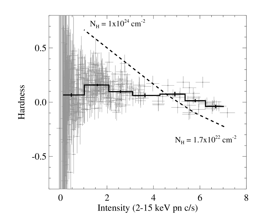
Figure 9.— Hardness-Intensity diagram for IGR J16207–5129. We used the 100 s time resolution light curves for the counts in the 5–15 keV band ($C_{hard}$) and the 2–5 keV band ($C_{soft}$). The hardness is defined as ($C_{hard}$–$C_{soft}$)/($C_{hard}$+$C_{soft}$). In addition to the individual 100 s points, which are grey in color, the averages in seven intensity bins are shown (the black histogram). The dashed line shows the hardness-intensity relationship expected if the change in count rate was due only to a change in column density.

To investigate which spectral parameters do change with intensity, we used the 0.4–15 keV pn light curve to divide the pn and MOS data into spectra at four intensity levels: 4–8 pn c/s, 2–4 pn c/s, 1–2 pn c/s, and 0–1 pn c/s. We used all of the data from the first 39 ks of the observation and obtained pn exposure times of 2,485 s, 6,177 s, 8,520 s, and 9,940 s and MOS exposure times of 3,412 s, 8,482 s, 11,700 s, and 13,650 s for the four intensity levels, respectively. In fitting these spectra, we simplified the two power-law model by requiring the same $\Gamma$ for both power-laws, which is equivalent to using a model where a fraction, $f$, of the power-law component is absorbed both by interstellar material and by the extra material local to the source, while a fraction, 1–$f$ is absorbed only by interstellar material. Table 2 shows the parameters obtained for the total spectrum and also for each of the four intensity levels, and Figure 10 shows the unfolded spectra for the four levels. While we performed all of the fits with pn and MOS spectra, Figure 10 shows only the pn spectra for clarity.

One interesting result that we obtain from the spectral parameters shown in Table 2 is that, at $N_{\rm H}=(6.4\pm 0.4)\times 10^{22}$ cm^-2, the column density for the highest intensity level is significantly less that for the lower levels. This spectrum is dominated by the flare that occurs during the first 3,000 s of the observation, and this indicates that lower $N_{\rm H}$ is the reason that this flare is softer. The parameters also indicate that there are two reasons why the spectrum is softer during the deepest dips. First, the power-law index indicates that the source gradually softens toward the lower levels, going from $\Gamma=1.06\pm 0.05$ at 4–8 c/s to $1.30\pm 0.12$ at 0–1 c/s. Secondly, the parameters and the spectra shown in Figure 10 indicate that the flux of the soft excess does not decrease as much as the flux of the primary power-law component. Between 2–4 c/s and 0–1 c/s, the flux of the primary power-law component changes by a factor of $5.1\pm 0.5$ while the flux of the soft excess changes by a factor of $2.0\pm 0.5$. The iron line parameters show that the equivalent width of the iron line is consistent with being constant while the flux of the line changes with the continuum flux.

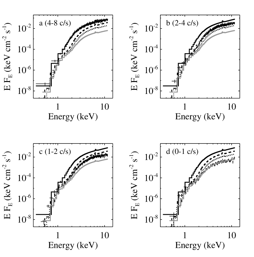
Figure 10.— Unfolded pn energy spectra after dividing the data into the following different intensity levels: (a) 4–8 pn c/s; (b) 2–4 pn c/s; (c) 1–2 pn c/s; and (d) 0–1 pn c/s. In each panel, the best fit partial covering fraction models are plotted for all four intensity levels.

4. Discussion

4.1. Is IGR J16207–5129 an Obscured HMXB?

While the Chandra position and the optical/IR spectroscopy leave essentially no doubt that IGR J16207–5129 is an HMXB, it has not been entirely clear whether the column density is high enough to require that part of the absorbing material is local to the source or not. The only other soft X-ray measurement besides the one reported here is the Chandra observation, and Tomsick et al. (2006) reported a value of $N_{\rm H}=(3.7^{+1.4}_{-1.2})\times 10^{22}$ cm^-2 (90% confidence errors), while many of the obscured HMXBs have column densities in excess of $10^{23}$ cm^-2. When one considers atomic and molecular hydrogen, the total Galactic column density is near $2.4\times 10^{22}$ cm^-2 (Dickey & Lockman, 1990; Dame, Hartmann & Thaddeus, 2001; Tomsick et al., 2008), so the Chandra measurement is only marginally higher than the Galactic value.

However, the value that we measure with XMM-Newton is substantially higher, $N_{\rm H}=(1.19^{+0.06}_{-0.05})\times 10^{23}$ cm^-2, which is significantly in excess of the Galactic value. To check on whether the difference between the Chandra and XMM-Newton measurements is related to variability in the column density, we re-analyzed the Chandra spectrum. In our previous Chandra analysis (Tomsick et al., 2006), we used the Anders & Grevesse (1989) rather than Wilms, Allen & McCray (2000) abundances, and we fitted the spectrum with only a single power-law. First, we find that when we use the Wilms, Allen & McCray (2000) abundances and re-fit the Chandra spectrum, we obtain a value of $N_{\rm H}=(5.4^{+2.1}_{-1.7})\times 10^{22}$ cm^-2, which is already somewhat higher than found in the previous analysis. Second, the quality of the Chandra spectrum does not allow for the detection of the soft excess, but we re-fitted the Chandra spectrum after including a soft excess with the values of $N_{\rm H}$ and $\Gamma$ measured with XMM-Newton (see Table 1). This fit gives values for the primary power-law component of $\Gamma=0.7\pm 0.7$ and $N_{\rm H}=7.9^{+4.4}_{-3.2}\times 10^{22}$ cm^-2, which are both consistent with the values measured with XMM-Newton.

Thus, the Chandra spectrum allows for the possibility that IGR J16207–5129 is an obscured HMXB while the XMM-Newton spectrum constrains $N_{\rm H}$ to be significantly higher than the Galactic value, requiring that the source is an obscured HMXB. With XMM-Newton, we see that the $N_{\rm H}$ can change, with the first 3,000 s of the observation having $N_{\rm H}=(6.4\pm 0.4)\times 10^{22}$ cm^-2, while the $N_{\rm H}$ was about a factor of two higher for the rest of the observation. The Chandra spectrum is consistent with either level. Even at the highest $N_{\rm H}$ seen by XMM-Newton, the amount of local absorbing material is certainly not as much as seen in some of the most extreme systems like IGR J16318–4848, which has $N_{\rm H}=2\times 10^{24}$ cm^-2. This is consistent with optical and IR observations which have shown P Cygni profiles, forbidden emission lines (indicating a supergiant B[e] spectral type), and IR excesses from local material for IGR J16318–4848 (Filliatre & Chaty, 2004; Moon et al., 2007; Rahoui et al., 2008) but not for IGR J16207–5129 (Negueruela & Schurch, 2007; Nespoli, Fabregat & Mennickent, 2008; Rahoui et al., 2008).

4.2. Comparison to other HMXBs Lacking Pulsations

With the results of our timing study, IGR J16207–5129 joins a relatively short list of accreting HMXBs that show very hard energy spectra, resembling known neutron star HMXBs, but that do not seem to exhibit pulsations (at least in the expected frequency range). One example is 4U 1700–377, which has an extremely massive and luminous O6.5 Iaf+ companion in a 3.41 day orbit with the compact object. The properties of this source as seen by XMM-Newton are remarkably similar to those of IGR J16207–5129 (van der Meer et al., 2005). Light curves with 10 s time resolution show flares and dips where the flux changes by factors of at least 5 on ks time scales. While the spectral analysis was limited to the fainter time periods because of photon pile-up, spectral fits show a direct component with a hard power-law index ($\Gamma=1.08$–1.87 for the “low-flux” spectrum, depending on the exact model used) and a high level of absorption ($N_{\rm H}=6.8\times 10^{22}$ cm^-2 to $N_{\rm H}=2.0\times 10^{23}$ cm^-2) along with a soft excess. While the light curves for 4U 1700–377 and IGR J16207–5129 are somewhat unusual in their extreme variability on long time scales, it should be noted that many pulsating HMXBs (e.g., Vela X-1 and GX 301–2) also show very similar energy spectra to those described here, with hard primary power-law components and soft excesses (Nagase, 1989).

A comparison of the power spectra of 4U 1700–377 and IGR J16207–5129 show similarities also. The typical power spectrum of an HMXB pulsar has 3 parts: A relatively flat portion at frequencies below the pulsation frequency; a region where the pulsations, harmonics, and sometimes quasi-periodic oscillations (QPOs) are observed, and a higher frequency region where the power spectrum can be described as a power-law with a slope of 1.4–2.0 (Belloni & Hasinger, 1990; Hoshino & Takeshima, 1993; Chakrabarty et al., 2001). However, a uniform study of 12 HMXBs with EXOSAT indicated that 4U 1700–377 (and, interestingly, Cyg X-3) deviated from this pattern by showing only a steep power-law in the 0.002–1 Hz frequency range (Belloni & Hasinger, 1990), like IGR J16207–5129. Belloni & Hasinger (1990) quote 0.008–29 Hz integrated rms noise levels for 4U 1700–377 between 6 and 12%, and if we recalculate the IGR J16207–5129 noise level for this frequency range, we obtain 11.7%$\pm$2.7%.

While there are many similarities between these two sources, one possible difference is that the average luminosity of 4U 1700–377 is probably higher. To avoid model-dependent flux measurements, we compare the average 20–40 keV flux measurements made by INTEGRAL. For 4U 1700–377, Bird et al. (2007) quote a value of $208.1\pm 0.1$ millicrab compared to $3.3\pm 0.1$ millicrab for IGR J16207–5129. The distance to 4U 1700–377 is estimated at 1.9 kpc (Ankay et al., 2001), so the ratio of fluxes for the two sources would imply a distance of $\sim$15 kpc for IGR J16207–5129 if their 20–40 keV luminosities were the same, which is at the very upper limit of the distance range derived by Nespoli, Fabregat & Mennickent (2008). At the best estimate for the IGR J16207–5129 distance, 6.1 kpc, the luminosity of IGR J16207–5129 would be about 6 times lower than 4U 1700–377. At a distance of 6.1 kpc, the average IGR J16207–5129 20–40 keV luminosity is $1.1\times 10^{35}$ ergs s^-1, and the average 0.5–10 keV unabsorbed luminosity is $1.6\times 10^{35}$ ergs s^-1.

Despite soft X-ray spectra that are similar to neutron star HMXBs, the nature of the compact object is still unclear for both 4U 1700–377 and IGR J16207–5129 because of the lack of X-ray pulsations. One reason that the black hole possibility has been taken seriously for 4U 1700–377 is that the compact object mass has been measured to be $2.44\pm 0.27$ $\rm\,M_{\mathord{\odot}}$ (Clark et al., 2002), which is significantly higher than the values close to 1.4$\rm\,M_{\mathord{\odot}}$ measured for most neutron stars (Thorsett & Chakrabarty, 1999), and could indicate that 4U 1700–377 harbors a low mass black hole. Obtaining a compact object mass measurement for IGR J16207–5129 would certainly be interesting and may be feasible as it is relatively bright in the optical and IR (see §$1$). However, the mass measurement would be challenging because accurate spectroscopy would be required to measure the massive B1 Ia companion’s radial velocity curve. Rather than black holes, these sources may harbor very slowly rotating neutron stars. Several such X-ray binaries are known: IGR J16358–4726 with its 1.64 hr pulsations (Patel et al., 2004); 2S 0114+650 with its 2.7 hr pulsations and B1 Ia spectral type (Farrell et al., 2008, and references therein), which is the same spectral type as IGR J16207–5129; 4U 1954+319 with its likely 5 hr pulsations (Mattana et al., 2006); and 1E 161348–5055.1 with its likely 6.7 hr pulsations (De Luca et al., 2006). With our $\sim$12 hr XMM-Newton observation of IGR J16207–5129, we can rule out pulsation periods in the $\sim$1–2 hr range but probably not in the $\mathrel{\lower 3.44444pt\hbox{\hbox to0.0pt{$\sim$\hss}\raise 3.87495pt\hbox{$>$} }}$4 hr range.

Another HMXB with a neutron star-like spectrum that has been well-studied without detecting pulsations is 4U 2206+54. This system has an O9.5 V or O9.5 III companion (Ribó et al., 2006) and a 9.6 or 19.25 day orbital period (Corbet, Markwardt & Tueller, 2007). Like IGR J16207–5129, its X-ray emission is highly variable (Masetti et al., 2004), but its energy spectrum is significantly different, showing no evidence for local absorption. Its $10^{-3}$–1 Hz power spectrum is dominated by strong red (i.e., power-law) noise (Negueruela & Reig, 2001; Torrejón et al., 2004; Blay et al., 2005), which is similar to IGR J16207–5129 and 4U 1700–377. However, for 4U 2206+54, the possible detection of a cyclotron line at $\sim$30 keV provides some additional evidence that the compact object is a neutron star (Torrejón et al., 2004; Blay et al., 2005). If confirmed, this would indicate that the lack of pulsations and the red noise power spectrum should not be taken as evidence for a black hole. Rather, the non-detections of pulsations could be related to a system geometry where, e.g., the neutron star magnetic and spin axes are nearly aligned, or the non-detections could be due to spin periods that are longer than the duration of the observations.

Finally, it is worth noting that several IGR HMXBs besides IGR J16207–5129 have not yet shown X-ray pulsations. IGR J19140+0951 has similarities to IGR J16207–5129, with a B0.5 I spectral type, a high level of obscuration (although the level depends on orbital phase), and a soft excess (see Prat et al., 2008, and references therein). IGR J16318–4848 (see §$4.1$) also has not exhibited pulsations despite a high level of X-ray variability that has been seen in several soft X-ray observations. Although the apparent lack of pulsations may be due to the fact that the timing properties of these sources have not been very well-studied yet, it is possible that the IGR HMXBs include a population of systems with black holes or very slowly rotating neutron stars.

4.3. Soft Excess and Iron Line

The presence of a soft excess and emission lines are very common in both pulsating and non-pulsating obscured HMXBs. In addition to iron lines, some sources (e.g., Vela X-1 and 4U 1700–377) have emission lines from Si, Ne, etc. in the 0.5–3 keV range, making up at least part of the soft excess (Watanabe et al., 2006; Boroson et al., 2003; van der Meer et al., 2005). Although our spectral analysis does not allow us to definitively rule out other models besides a power-law (e.g., Bremsstrahlung or black-body) for the soft excess, the fact using a power-law leads to a power-law index that is consistent with the value of $\Gamma$ for the primary power-law components allows for two possible physical interpretations. One possibility is the partial covering of the power-law source by absorbing material (likely the stellar wind), which is the scenario envisioned for the spectral fits described in §$3.2.2$. Another possible explanation is that the soft excess emission originates as part of the primary power-law component, but it is scattered in the stellar wind. In this picture, the fact that the soft excess has a much lower column density than the primary component would indicate that the photons that are part of the soft excess come from the edge (i.e., within one optical depth of the edge) of the stellar wind.

Although it is not clear whether any of the IGR J16207–5129 soft excess comes from emission lines, the fact that the flux of the Fe K$\alpha$ line at 6.4 keV correlates with the overall source flux (i.e., the equivalent width is consistent with being constant) is different from Vela X-1 and 4U 1700–377, which both show lines with very large equivalent widths at low luminosities. Regardless of the presence (or not) of lower energy lines in IGR J16207–5129, the energy of the iron line indicates a low ionization state implies that the line originates in cool material. One possible location for the cool material is an accretion disk around the IGR J16207–5129 compact object; however, many HMXBs with strong stellar winds have compact objects that accrete directly from the wind with little or no disk accretion. The equivalent width of $42\pm 12$ eV that we measure for the IGR J16207–5129 iron line is consistent with simulations in which a spherical distribution of cold matter with solar abundances and $N_{\rm H}\sim 10^{23}$ cm^-2 is illuminated by a central X-ray source (Matt, 2002), and this is also true for several other IGR HMXBs (Walter et al., 2006). Although it is not obvious that the matter in a stellar wind will be cold (i.e., neutral), it has been suggested that the wind might be a clumpy two-phase medium with cool, dense regions that are responsible for the emission lines along with hot, highly-ionized regions (van der Meer et al., 2005, and references therein). The partial covering model that we use to fit the IGR J16207–5129 continuum would also be consistent with absorption of the X-ray source by a clumpy wind.

5. Summary and Conclusions

The XMM-Newton observation of IGR J16207–5129 confirms that it is a member of the group of obscured IGR HMXBs. We measure a column density of $N_{\rm H}=(1.19^{+0.06}_{-0.05})\times 10^{23}$ cm^-2 for the average spectrum. We find that the column density could have been that high during the only previous soft X-ray observation of this source with Chandra, but a detailed spectral analysis of the XMM-Newton data shows that $N_{\rm H}$ can vary by a factor of $\sim$2. We detect an iron line in the energy spectrum, and its strength is consistent with what is expected for a spherical distribution of material with the measured $N_{\rm H}$ around the compact object. Although the X-ray spectrum is similar to those seen from other neutron star HMXBs with a hard primary power-law component and a soft excess, we do not detect the pulsations that might be expected if the compact object is a neutron star.

A detailed comparison between IGR J16207–5129 and another apparently non-pulsating HMXB, 4U 1700–377, shows strong similarities in spectral and timing properties. Most notably, the power spectra of both sources can be described as a single power-law down to $10^{-3}$-$10^{-4}$ Hz. Since pulsating HMXBs show power spectra that break near the pulsation frequency, it is possible that both of these sources harbor very slowly rotating neutron stars (although the possibility that the compact object is a black hole cannot be ruled out entirely). We note that several of the IGR HMXBs are either known to harbor slowly rotating neutron stars or may harbor slowly rotating neutron stars in cases where pulsations have not been detected. It is possible that in addition to uncovering obscured HMXBs, the HMXBs that INTEGRAL is uncovering tend to contain slow rotators.

Table 1Spectral Results

Parameter	Value
Primary Power-Law Component
$N_{\rm H}$	$(1.19^{+0.06}_{-0.05})\times 10^{23}$ cm-2
$\Gamma$	$1.15^{+0.07}_{-0.05}$
$F_{PL}$ (unabsorbed, 0.5–10 keV)	$(3.68\pm 0.10)\times 10^{-11}$ ergs cm-2 s-1
Soft Excess
$N_{\rm H}$	$1.7\times 10^{22}$ cm-2 (fixed)
$\Gamma$	$0.9^{+0.5}_{-0.4}$
$F_{PL}$	$(1.8^{+1.0}_{-0.7})\times 10^{-12}$
Iron Line Parameters
$N_{\rm H}$	$1.7\times 10^{22}$ cm-2 (fixed)
$E_{\rm line}$	$6.39\pm 0.03$ keV
$\sigma_{\rm line}$	$<$0.12 keV
$N_{\rm line}$	$(1.6^{+0.5}_{-0.4})\times 10^{-5}$ photons cm-2 s-1
Equivalent Width	$42\pm 12$ eV
$\chi^{2}/\nu$	1402/1300

Table 2Spectral Results with the Partial Covering Model vs. Intensity

	Value	Value	Value	Value	Value
Parameter	(all rates)	(4–8 c/s)	(2–4 c/s)	(1–2 c/s)	(0–1 c/s)
Partially Absorbed Power-law Parameters
$N_{\rm H}$ ($\times 10^{23}$ cm-2)	$1.00^{+0.04}_{-0.05}$	$0.64\pm 0.04$	$1.14\pm 0.06$	$1.31\pm 0.09$	$1.24\pm 0.13$
$\Gamma$	$1.13\pm 0.02$	$1.06\pm 0.05$	$1.15\pm 0.06$	$1.21\pm 0.08$	$1.30\pm 0.12$
$f$	$0.963\pm 0.003$	$0.964\pm 0.008$	$0.980\pm 0.004$	$0.971\pm 0.005$	$0.951^{+0.009}_{-0.011}$
$F_{PL}$	$3.84^{+0.07}_{-0.04}$	$11.2\pm 0.3$	$6.06^{+0.24}_{-0.11}$	$3.33^{+0.18}_{-0.17}$	$1.22^{+0.12}_{-0.10}$
$F_{PPL}=F_{PL}f$	$3.70^{+0.07}_{-0.04}$	$10.8\pm 0.3$	$5.94^{+0.24}_{-0.11}$	$3.23\pm 0.17$	$1.16^{+0.11}_{-0.10}$
$F_{SE}=F_{PL}(1-f)$	$0.142\pm 0.012$	$0.40\pm 0.09$	$0.12\pm 0.02$	$0.10\pm 0.02$	$0.060\pm 0.013$
Iron Line Parameters
$E_{\rm line}$ (keV)	$6.39\pm 0.03$	$6.44\pm 0.08$	$6.33\pm 0.05$	$6.41^{+0.07}_{-0.06}$	$6.39^{+0.10}_{-0.09}$
$\sigma_{\rm line}$ (keV)	$0.06^{+0.03}_{-0.06}$	0.06	0.06e	0.06e	0.06e
$N_{\rm line}$	$1.6^{+0.5}_{-0.7}$	$4.9^{+2.1}_{-3.3}$	$2.5^{+0.8}_{-1.1}$	$1.0\pm 0.6$	$0.48^{+0.36}_{-0.32}$
EW (eV)	$42^{+13}_{-18}$	$44^{+18}_{-30}$	$43^{+14}_{-19}$	$32\pm 19$	$44^{+33}_{-29}$
$\chi^{2}/\nu$	1402/1301	489/468	528/503	432/397	232/193

References

- Anders & Grevesse (1989) Anders, E., & Grevesse, N., 1989, Geochimica et Cosmochimica Acta, 53, 197
- Ankay et al. (2001) Ankay, A., Kaper, L., de Bruijne, J. H. J., Dewi, J., Hoogerwerf, R., & Savonije, G. J., 2001, A&A, 370, 170
- Balucinska-Church & McCammon (1992) Balucinska-Church, M., & McCammon, D., 1992, ApJ, 400, 699
- Belloni & Hasinger (1990) Belloni, T., & Hasinger, G., 1990, A&A, 230, 103
- Bird et al. (2007) Bird, A. J., et al., 2007, ApJS, 170, 175
- Blay et al. (2005) Blay, P., Ribó, M., Negueruela, I., Torrejón, J. M., Reig, P., Camero, A., Mirabel, I. F., & Reglero, V., 2005, A&A, 438, 963
- Boroson et al. (2003) Boroson, B., Vrtilek, S. D., Kallman, T., & Corcoran, M., 2003, ApJ, 592, 516
- Chakrabarty et al. (2001) Chakrabarty, D., Homer, L., Charles, P. A., & O’Donoghue, D., 2001, ApJ, 562, 985
- Chaty et al. (2008) Chaty, S., Rahoui, F., Foellmi, C., Tomsick, J. A., Rodriguez, J., & Walter, R., 2008, A&A, 484, 783
- Clark et al. (2002) Clark, J. S., Goodwin, S. P., Crowther, P. A., Kaper, L., Fairbairn, M., Langer, N., & Brocksopp, C., 2002, A&A, 392, 909
- Corbet, Markwardt & Tueller (2007) Corbet, R. H. D., Markwardt, C. B., & Tueller, J., 2007, ApJ, 655, 458
- Dame, Hartmann & Thaddeus (2001) Dame, T. M., Hartmann, D., & Thaddeus, P., 2001, ApJ, 547, 792
- De Luca et al. (2006) De Luca, A., Caraveo, P. A., Mereghetti, S., Tiengo, A., & Bignami, G. F., 2006, Science, 313, 814
- Dickey & Lockman (1990) Dickey, J. M., & Lockman, F. J., 1990, ARA&A, 28, 215
- Farrell et al. (2008) Farrell, S. A., Sood, R. K., O’Neill, P. M., & Dieters, S., 2008, MNRAS, 389, 608
- Filliatre & Chaty (2004) Filliatre, P., & Chaty, S., 2004, ApJ, 616, 469
- Grove et al. (1998) Grove, J. E., Johnson, W. N., Kroeger, R. A., McNaron-Brown, K., Skibo, J. G., & Phlips, B. F., 1998, ApJ, 500, 899
- Hoshino & Takeshima (1993) Hoshino, M., & Takeshima, T., 1993, ApJ, 411, L79
- in ’t Zand (2005) in ’t Zand, J. J. M., 2005, A&A, 441, L1
- Leahy et al. (1983) Leahy, D. A., Darbro, W., Elsner, R. F., Weisskopf, M. C., Kahn, S., Sutherland, P. G., & Grindlay, J. E., 1983, ApJ, 266, 160
- Lutovinov et al. (2005) Lutovinov, A., Revnivtsev, M., Gilfanov, M., Shtykovskiy, P., Molkov, S., & Sunyaev, R., 2005, A&A, 444, 821
- Masetti et al. (2004) Masetti, N., Dal Fiume, D., Amati, L., Del Sordo, S., Frontera, F., Orlandini, M., & Palazzi, E., 2004, A&A, 423, 311
- Masetti et al. (2006) Masetti, N., et al., 2006, A&A, 459, 21
- Matt (2002) Matt, G., 2002, MNRAS, 337, 147
- Mattana et al. (2006) Mattana, F., Götz, D., Falanga, M., Senziani, F., de Luca, A., Esposito, P., & Caraveo, P. A., 2006, A&A, 460, L1
- McClintock & Remillard (2006) McClintock, J. E., & Remillard, R. A., 2006, Black hole binaries, in Compact stellar X-ray sources. Edited by Walter Lewin & Michiel van der Klis: Cambridge University Press, 157
- Moon et al. (2007) Moon, D.-S., Kaplan, D. L., Reach, W. T., Harrison, F. A., Lee, J.-E., & Martin, P. G., 2007, ApJ, 671, L53
- Nagase (1989) Nagase, F., 1989, PASJ, 41, 1
- Nagase et al. (1986) Nagase, F., Hayakawa, S., Sato, N., Masai, K., & Inoue, H., 1986, PASJ, 38, 547
- Negueruela & Reig (2001) Negueruela, I., & Reig, P., 2001, A&A, 371, 1056
- Negueruela & Schurch (2007) Negueruela, I., & Schurch, M. P. E., 2007, A&A, 461, 631
- Negueruela et al. (2006) Negueruela, I., Smith, D. M., Reig, P., Chaty, S., & Torrejón, J. M., 2006, in ESA SP-604: The X-ray Universe 2005, ed. A. Wilson, 165
- Nespoli, Fabregat & Mennickent (2008) Nespoli, E., Fabregat, J., & Mennickent, R. E., 2008, A&A, 486, 911
- Patel et al. (2004) Patel, S. K., et al., 2004, ApJ, 602, L45
- Prat et al. (2008) Prat, L., Rodriguez, J., Hannikainen, D. C., & Shaw, S. E., 2008, MNRAS, 389, 301
- Rahoui et al. (2008) Rahoui, F., Chaty, S., Lagage, P.-O., & Pantin, E., 2008, A&A, 484, 801
- Ribó et al. (2006) Ribó, M., Negueruela, I., Blay, P., Torrejón, J. M., & Reig, P., 2006, A&A, 449, 687
- Sguera et al. (2006) Sguera, V., et al., 2006, ApJ, 646, 452
- Strüder et al. (2001) Strüder, L., et al., 2001, A&A, 365, L18
- Thorsett & Chakrabarty (1999) Thorsett, S. E., & Chakrabarty, D., 1999, ApJ, 512, 288
- Tomsick et al. (2006) Tomsick, J. A., Chaty, S., Rodriguez, J., Foschini, L., Walter, R., & Kaaret, P., 2006, ApJ, 647, 1309
- Tomsick et al. (2008) Tomsick, J. A., Chaty, S., Rodriguez, J., Walter, R., & Kaaret, P., 2008, ApJ, 685, 1143
- Tomsick et al. (2004) Tomsick, J. A., Lingenfelter, R., Corbel, S., Goldwurm, A., & Kaaret, P., 2004, in ESA SP-552: 5th INTEGRAL Workshop on the INTEGRAL Universe, 413
- Torrejón et al. (2004) Torrejón, J. M., Kreykenbohm, I., Orr, A., Titarchuk, L., & Negueruela, I., 2004, A&A, 423, 301
- Turner et al. (2001) Turner, M. J. L., et al., 2001, A&A, 365, L27
- van der Klis (1989) van der Klis, M., 1989, Fourier Techniques in X-ray Timing, in Timing Neutron Stars, Eds. H. Ögelman and E.P.J. van den Heuvel: Published by Kluwer Academic/Plenum Publishers, 27
- van der Meer et al. (2005) van der Meer, A., Kaper, L., di Salvo, T., Méndez, M., van der Klis, M., Barr, P., & Trams, N. R., 2005, A&A, 432, 999
- Walter et al. (2004) Walter, R., et al., 2004, The Astronomer’s Telegram, 229
- Walter & Zurita Heras (2007) Walter, R., & Zurita Heras, J., 2007, A&A, 476, 335
- Walter et al. (2006) Walter, R., et al., 2006, A&A, 453, 133
- Watanabe et al. (2006) Watanabe, S., et al., 2006, ApJ, 651, 421
- Wilms, Allen & McCray (2000) Wilms, J., Allen, A., & McCray, R., 2000, ApJ, 542, 914
- Winkler et al. (2003) Winkler, C., et al., 2003, A&A, 411, L1