Cross-Correlation between Damped Ly$\alpha$ Systems and Lyman Break Galaxies in Cosmological SPH Simulations

Abstract

We calculate the cross-correlation function (CCF) between damped Ly-$\alpha$ systems (DLAs) and Lyman break galaxies (LBGs) using cosmological hydrodynamic simulations at $z=3$. We compute the CCF with two different methods. First, we assume that there is one DLA in each dark matter halo if its DLA cross section is non-zero. In our second approach we weight the pair-count by the DLA cross section of each halo, yielding a cross-section-weighted CCF. We also compute the angular CCF for direct comparison with observations. Finally, we calculate the auto-correlation functions of LBGs and DLAs, and their bias against the dark matter distribution. For these different approaches, we consistently find that there is good agreement between our simulations and observational measurements by Cooke et al. (2006a) and Adelberger et al. (2005). Our results thus confirm that the spatial distribution of LBGs and DLAs can be well described within the framework of the concordance $\Lambda$CDM model. We find that the correlation strengths of LBGs and DLAs are consistent with the actual observations, and in the case of LBGs it is higher than would be predicted by low-mass galaxy merger models.

1 Introduction

According to the cold dark matter (CDM) model of structure formation, the spatial distribution of galaxies can be understood as a result of gravitational instability of density fluctuations in the CDM, and the dark matter halo mass function can be well described by analytic models (Sheth & Tormen, 1999). More precisely, hierarchical CDM models predict that the massive galaxies at high redshift (hereafter high-$z$) are clustered together in high-density regions, while low-mass galaxies tend to be more evenly spaced (Kaiser, 1984; Bardeen et al., 1986). Under the assumption that galaxies are produced from primordial density fluctuations owing to gravitational instability, one can estimate the average mass of galaxy host haloes based on clustering data. For example, Adelberger et al. (1998) estimated the typical halo mass of LBGs at $z\sim 3$ to be $10^{10.8}M_{\odot}\lesssim M_{\rm halo}\lesssim 10^{12}\,M_{\odot}$ from observations of their auto-correlation function (ACF).

Damped Lyman-$\alpha$ systems (DLAs), defined as quasar absorption systems with column density of ${N_{\rm HI}}>2\times 10^{20}$ atoms cm^-2 (Wolfe et al., 1986), probe the H i   gas associated with high-$z$ galaxies. Since stars are hardly formed in warm ionized gas and are tightly correlated with cold neutral clouds, the amount of H i   gas is very important, being the precursor of molecular clouds (Wolfe et al., 2003). DLAs dominate the H i   content of the Universe at $z\simeq 3$ and contain a sufficient amount of H i   gas mass to account for a large fraction of the present-day stellar mass (Storrie-Lombardi & Wolfe, 2000). The gas kinematics and chemical abundances of DLAs can be measured and are documented in detail. However, the masses of DLA host haloes (hereafter DLA haloes) remain poorly constrained, because only about $20\%$ of quasars exhibit DLA absorption per unit redshift (Nagamine et al., 2007), and the scattered distribution of DLAs in quasar sight lines precludes the use of DLAs as tracers of dark matter halo mass.

Alternatively, the mass of DLA haloes can be probed by the cross-correlation between DLAs and a galaxy population whose clustering and halo mass are well understood. Cooke et al. (2006a, b) used 211 LBG spectra and 11 DLAs to measure the three dimensional (3-D) LBG ACF and DLA-LBG CCF (see also Gawiser et al., 2001; Bouche & Lowenthal, 2004; Bouche et al., 2005). Their analysis started by counting the number of LBGs in 3-D cylindrical bins centred on each of 11 DLAs, following the method of Adelberger et al. (2003). They detected a statistically significant result of DLA-LBG CCF, and estimated an average DLA halo mass of $\langle M_{\rm DLA}\rangle\approx 10^{11.2}M_{\odot}$, assuming a single galaxy per halo.

On the theoretical side, Nagamine et al. (2007) calculated the average DLA halo mass using a series of cosmological hydrodynamic simulations with different box sizes, resolution and feedback strengths. They found a mean DLA halo mass of $\langle M_{\rm DLA}\rangle=10^{12.4}\,M_{\odot}$ with their Q5 run which is somewhat larger than $\langle M_{\rm DLA}\rangle=10^{11.2}\,M_{\odot}$ of Cooke et al. (2006a). More recent work by Pontzen et al. (2008) showed that the DLA cross-section is predominantly provided by intermediate mass haloes, $10^{9}<M_{\rm vir}/M_{\odot}<10^{11}$. These results motivate us to further examine the distribution of DLAs relative to that of LBGs. In this paper, we compute the DLA-LBG CCF in cosmological SPH simulations, using the sample of LBGs and DLAs obtained by Nagamine et al. (2004a, b). We compare our results with the observational results by Adelberger et al. (2005) and Cooke et al. (2006a, b).

Our paper is organized as follows. In Section 2, we briefly describe the features of our cosmological SPH simulations used in this paper. In Section 4 and Section 5, we describe and report the methodology, binning method, and the results for ‘unweighted’ and ‘weighted’ DLA-LBG CCF, respectively. We then discuss the projected angular CCF for the direct comparison with observational result by Cooke et al. (2006a, b) in Section 6. The ACFs of LBG-LBG and DLA-DLA are discussed in Subsections 7.1 and 7.2, while the bias results are reported in Section 8. Finally, we discuss the implications of our work in Section 9.

2 Simulations

In this paper, we use two different cosmological smoothed particle hydrodynamics (SPH) simulations (Springel & Hernquist, 2003b) performed with the GADGET-2 code (Springel, 2005). The simulation parameters of the two runs (named D5 and G5) are summarised in Table 1. The same set of runs has been used by Nagamine et al. (2004b, a, 2007) to study the global properties of DLAs, such as the DLA cross section, incidence rate, and H i   column density distribution functions.

The code we use is characterized by four main features. First, it uses the entropy-conserving formulation of SPH (Springel & Hernquist, 2002), which explicitly conserves entropy of the gas where appropriate. Second, highly overdense gas particles are treated with a sub-resolution model for the interstellar medium (ISM) (Springel & Hernquist, 2003a). The dense ISM is assumed to be made of a two-phase fluid consisting of cold clouds in pressure equilibrium with a hot ambient phase. Cold clouds grow by radiative cooling, and form the reservoir of baryons for star formation. Once star formation occurs, the resulting supernovae (SNe) deposit energy into the ISM, heating the hot gas environment, evaporating cold clouds, and transferring cold gas back into the ambient phase. This establishes a self-regulation cycle for star formation in the ISM, Additionally, the simulation keeps track of metal abundance and the dynamical transport of metals. Metals are produced by stars and returned into the gas by SNe.

Third, a model for galactic winds is included to study the effects of outflows on DLAs, galaxies, and intergalactic medium (IGM). In this model, gas particles are driven out of dense star-forming medium by assigning an extra momentum in random directions (Springel & Hernquist, 2003a). It is assumed that the wind mass-loss rate is proportional to the star formation rate, and the wind takes a fixed fraction of the SN energy. For the D5 and G5 runs, a strong wind speed of 484 km s^-1 is adopted (as opposed to the ’weak’ wind speed of 242 km s^-1; Springel & Hernquist (2003a)). The dependence of the wind models on DLA properties was discussed in detail by Nagamine et al. (2007). Fourth, the code includes radiative cooling and heating with a uniform UV background of a modified Haardt & Madau (1996) spectrum (Katz et al., 1996; Davé et al., 1999), where the reionisation takes place at $z\simeq 6$.

We identify simulated galaxies by grouping the star particles using a simplified variant of the SUBFIND algorithm proposed by Springel et al. (2001). This code computes an adaptively smoothed baryonic density field for all star and gas particles, and identifies the centres of individual galaxies as isolated density peaks. It finds the full extent of these galaxies by processing the gas and star particles in the order of declining density, adding particles one by one to the galaxies.

Once the simulated galaxies and consituent particles are identified, we then calculate the luminosity and spectrum of individual star particles using the mass, formation time, and metallicity using the population synthesis code GALAXEV03 (Bruzual & Charlot, 1993) that assumes the Salpeter initial mass function with a mass range of $[0.1,125]\,M_{\odot}$. The spectrum of each galaxy is obtained by coadding the spectrum of constituent star particles, and the broad-band colours are computed by convolving with filter functions. The LBGs are then selected based on the $U_{n}GR$ colour selection criteria as described in Nagamine et al. (2004).

Run	$L_{\rm box}$	${N_{\rm p}}$	$m_{\rm DM}$	$m_{\rm gas}$	$\epsilon$
D5	33.75	$2\times 324^{3}$	$8.15\times 10^{7}$	$1.26\times 10^{7}$	4.17
G5	100.0	$2\times 324^{3}$	$2.12\times 10^{9}$	$3.26\times 10^{8}$	12.3

Table 1: Simulations employed in this study. $N_{\rm P}$ is the initial number of gas and dark matter particles (hence $\times 2$). $m_{\rm DM}$ and $m_{\rm gas}$ are the masses of dark matter and gas particles in units of $\,h^{-1}{M_{\odot}}$, respectively. $\epsilon$ is the comoving gravitational softening length in units of $h^{-1}{\rm\,kpc}$, which is a measure of spatial resolution. All runs adopt a ‘strong’ galactic wind feedback model.

3 Outline of Methods

Before we present the results of our calculations, let us describe the series of method that we use to measure the correlations of DLAs and LBGs. First, we will examine the simplest case in Section 4, where we assume that there is only one DLA per halo at the center. We then discuss the DLA cross-section-weighted CCF in Section 5 to examine the effect of multiple DLA clouds in massive haloes. We compute these two cases using the three dimensional coordinates ($x,y,z$) of DLAs and LBGs. Next, to mimic the observational estimates of two dimensional angular CCF, we compute the angular CCF in Section 6. Finally we compute the auto correlation functions of DLAs and LBGs separately in Section 7, and discuss the biases and halo masses of DLAs and LBGs in Section 8.

4 DLA-LBG Cross-Correlation

The probability of finding an object 1 in volume $\delta V_{1}$ at a separation $r$ from a randomly chosen object 2 can be written as $\delta P=n_{1}\,[1+\xi_{12}(r)]\,\delta V_{1}$ (Peebles, 1980). The joint probability of finding an object 1 in volume 1 ($\delta V_{1}$) and an object 2 in volume 2 ($\delta V_{2}$) at a separation $r$ is defined as $\delta P=n_{1}n_{2}\,[1+\xi_{12}(r)]\,\delta V_{1}\delta V_{2},$ where $n_{1}$ and $n_{2}$ are the mean number densities of the two population. For the cross-correlation, we replace object 1 and 2 with DLA and LBG, then the joint probability between DLA and LBG is

$$\delta P=n_{\rm DLA}n_{\rm LBG}\,[1+\xi_{\rm DLA-LBG}(r)]\,\delta V_{\rm DLA}\delta V_{\rm LBG},$$ (1)

where $n_{\rm DLA}$ and $n_{\rm LBG}$ are the mean number densities of DLAs and LBGs, and $\xi_{\rm DLA-LBG}(r)$ is the cross-correlation function (CCF).

To estimate $\xi_{\rm DLA-LBG}(r)$, we use the method of Landy & Szalay (1993) and Cooke et al. (2006a):

$$\xi_{\rm DLA-LBG}(r)=$$

$$\frac{D_{\rm DLA}D_{\rm LBG}-D_{\rm DLA}R_{\rm LBG}-R_{\rm DLA}D_{\rm LBG}+R_{\rm DLA}R_{\rm LBG}}{R_{\rm DLA}R_{\rm LBG}},$$

where $D_{\rm DLA}D_{\rm LBG}$ is the number of pairs between the two data samples of DLAs and LBGs separated by a distance $r\pm\delta r$, and likewise for other terms. The notation “$R_{\rm DLA}$”, for example, represents the DLA sample that has random coordinate positions but with an equivalent number density as the original data sample “$D_{\rm DLA}$”.

Figure 1: DLA-LBG CCFs at $z=3$ calculated with the regular unweighted method (Equation LABEL:eq:xi01). The variance of CCFs computed with 100 different random seeds is shown with vertical errorbars, and the open square symbols are the mean of 100 trials. The blue dashed line is the least-square fit to the open square points. The red solid line and the short and long dashed lines are the angular and 3-D best-fitting power-laws of Cooke et al. (2006a, b), respectively, and the yellow shade is their 1-$\sigma$ error range for the angular CCF.

The method of identifying DLAs in our simulations is described in detail in Nagamine et al. (2004a) (see also Katz et al., 1996a; Hernquist et al., 1996). Briefly, we set up a cubic grid that completely covers each dark matter halo, with the grid-cell size equivalent to the gravitational softening length ‘$\epsilon$’ of each run. We then calculate the H i   column density ${N_{\rm HI}}$ of each pixel (i.e., a grid-cell on one of the planes) by projecting the H i   mass distribution, and identify those that exceed the DLA threshold of ${N_{\rm HI}}>2\times 10^{20}$ atoms cm^-2 as ‘DLA-pixels’. This method allows us to quantify the DLA cross-section ‘$\sigma_{\rm DLA}$’ of each halo, and the number of DLA-pixel is $N_{i}^{\rm DLA}=\sigma_{\rm DLA}/\epsilon^{2}$. Note that we have not made any corrections for the self-shielding of neutral gas in this work. Self-shielding may have significant impact at high H i   column densities, and we are currently investigating this issue with separate simulations (Nagamine et al., 2010).

Here we focus on the correlation signal at $r\gtrsim 0.4\,h^{-1}{\rm\,Mpc}$, because this is the scale probed by Cooke et al. (2006a, b). Therefore in this paper we are only concerned about the overall halo positions and not the exact locations of individual DLA-pixel within each halo. The $\sigma_{\rm DLA}$-weighted CCF will be discussed in Section 5.

First, we select the LBGs that are brighter than $R_{\rm AB}$=25.5 magnitude in the D5 and G5 runs. There are 30 (4030) LBGs in the D5 (G5) run. Nagamine et al. (2004) have shown that the brightest galaxies with $R_{\rm AB}<25.5$ in our simulations satisfy the $U_{n}GR$ colour selection criteria for LBGs (e.g., Steidel et al., 1999). Figure 2 of Nagamine et al. (2004) shows that the D5 run underestimates the number density of LBGs, while the G5 run agrees better with the observation.

There are 22616 (25683) DLA haloes with $\sigma_{\rm DLA}>0$ in the simulated volumes of the D5 (G5) run. The ‘random’ catalogues of LBGs and DLA haloes with random positions were created with a random number generator from Numerical Recipes (Press et al., 1992). The selected LBGs were paired with DLA haloes, and the number of pairs that reside in spherical shells of [$\log r,\log r+\Delta\log r$] were counted. The maximum pair separations probed for the D5 and G5 runs are 10 and $35\,h^{-1}{\rm\,Mpc}$, respectively, with 20 bins in a logarithmic scale of distance $r$. The periodic boundary condition was taken into account appropriately, and the pair-search was extended to the next adjacent box where needed.

We correct all $\xi(r)$ values by the integral constraint (IC). This correction owes to the finite size of the observed field-of-view, and it must be added to the computed correlation function as follows:

	Unweighted		$\sigma_{\rm DLA}$-weighted
Run	$r_{0}$	$\gamma$	$r_{0}$	$\gamma$
D5	2.66 $\pm$ 0.23	1.50 $\pm$ 0.17	3.37 $\pm$ 0.36	1.77 $\pm$ 0.21
G5	3.03 $\pm$ 0.04	1.64 $\pm$ 0.03	3.43 $\pm$ 0.06	1.66 $\pm$ 0.03

Table 2: Best-fitting power-law parameters of unweighted and $\sigma_{\rm DLA}$-weighted DLA-LBG CCFs at $z=3$. The correlation length $r_{0}$ is in units of $h^{-1}{\rm\,Mpc}$. The confidence limit statistics for this work are described in Section 5.1. For comparison, Cooke (private communication) obtained $r_{0}=2.91\pm 1.0\,h^{-1}{\rm\,Mpc}$ and $\gamma=1.21^{+0.6}_{-0.3}$ for the 3-D CCF calculated with spherical shells, and Cooke et al. (2006b) reported $r_{0}=3.32\pm 1.25\,h^{-1}{\rm\,Mpc}$ and $\gamma=1.74\pm 0.36$ for the angular CCF.

$$\xi^{\prime}(r)=\xi(r)+{\rm IC},$$ (3)

where $\xi^{\prime}(r)$ and $\xi(r)$ are the corrected and computed CCF (or ACF) respectively. Following the method described in Adelberger et al. (2005) and Lee et al. (2006), we calculate the value of IC and find that it changes $\xi(r)$ only slightly in our simulations, with IC $\sim 10^{-2}$ for the D5 run.

Figure 1 shows the DLA-LBG CCF computed with Eq. (LABEL:eq:xi01). We perform a least-square fit to the measured values with a power-law $\xi(r)=(r_{0}/r)^{\gamma}$, and find best-fitting parameters equal to $(r_{0}[h^{-1}{\rm\,Mpc}],\gamma)=(2.66\pm 0.23,1.50\pm 0.17)$ and $(3.03\pm 0.04,1.64\pm 0.03)$ for the D5 and G5 runs, respectively. The fits are shown by the blue long-dashed lines (see also Table 2), and the confidence limit statistics are described in Section 5.1.

Landy & Szalay (1993) showed that the variance of $\omega_{p}(r_{\theta})$ obtained from Monte Carlo calculations agrees quite well with the standard Poisson variance. Here, we follow their method outlined in their Section 5.2 and repeat the calculation of the CCF 100 times using different seeds for generating the random positions for the ‘random’ sample to examine the statistical variance of the measured CCF. The variance of 100 trials is shown as vertical errorbars, and the average of 100 trials is shown with the open square data points. The red solid line and the yellow shade represent the best-fitting result ($r_{0}=3.32\pm 1.25$ and $\gamma=1.74\pm 0.36$) and the 1-$\sigma$ errors of Cooke et al. (2006a, b) from their angular CCF result. The result of the G5 run agrees well with that of Cooke et al.’s, and its variance is small owing to a larger sample than in the D5 run. The result of the D5 run is somewhat shallower than that of the G5 run, which could simply owe to relatively small sample of LBGs in D5 and its small box-size.

Cooke et al. (2006a, b) published only the angular CCFs. However, they can also estimate the 3-D radial CCF using redshift information. The best-fitting parameters to the radial CCF by Cooke (private communication) using spherical shells is $r_{0}=3.39\pm 1.2\,h^{-1}{\rm\,Mpc}$ and $\gamma=1.61\pm 0.3$, which is shallower than the angular CCF results. As we will further discuss in Section 6, the method of Adelberger et al. (2003) adopts cylindrical shells at small distances, which have larger volumes than spherical shells. The cylindrical shell method uses long cylinders at small $r_{\theta}$ and captures all the potential LBGs near the DLAs, whereas the spherical bins do not. This effect seems to result in the slightly steeper $\gamma$ in Cooke et al. (2006b) compared to the above spherical shell case (Cooke; private communication). We regard the comparison to the angular CCF of Cooke et al. (2006b) as the primary one, because Cooke et al. argue that the angular CCF calculated by the method of Adelberger et al. (2003) is more robust than the 3-D radial calculation with spherical shells, and the values of ($r_{0}$, $\gamma$) derived from both CCFs should be equivalent theoretically (see Section 6).

Figure 2: DLA-LBG CCF at $z=3$ calculated by the $\sigma_{\rm DLA}$-weighted method (Equation LABEL:eq:xi02). The yellow shade shows the upper and lower limits of Cooke et al. (2006a, b)’s best-fitting power-laws. The variance of the CCF using 100 random seeds shown with vertical errorbars. The blue dashed lines are the best-fittings for this work, and the red solid line and the short and long dashed lines are, respectively, the angular and 3-D best-fitting power-laws of Cooke et al. (2006a, b).

5 $\sigma_{\rm DLA}$-weighted CCF

In Section 4, we calculated the CCF assuming that there is one DLA per halo. This assumption is valid as long as we are concerned with the CCF at scales of $r\gtrsim 300\,h^{-1}{\rm\,kpc}$. However, Nagamine et al. (2004b, Fig. 1) showed that the DLA clouds have extended distributions in massive dark matter haloes. Therefore, it may be more desirable to take the DLA cross-section of each halo into account when calculating the CCF, because the chance of finding a DLA in the actual observation is already cross-section weighted. Ideally, we would use all the DLA pixels and find pairs with the nearby LBGs, but this computation is prohibitively expensive owing to the large number of DLA pixels.

A simple way to achieve this is to weight the number of DLA-LBG pairs by the number of DLA-pixels of each halo. Since the displacement between DLA-pixels within a single halo is typically much smaller than the distance between LBG-DLA pairs, we do not count the individual pairs between LBG and DLA-pixels. Instead, we treat it as if all DLA-pixels are located at the halo centre, and weight each DLA-LBG pair-count by the number of DLA-pixels $N_{i}$ (hereafter we drop the superscript ‘DLA’ for simplicity) and compute the $\sigma_{\rm DLA}$-weighted CCF as

$$\xi_{\rm DLA-LBG}(r)={}$$

$${}\frac{\scriptstyle N_{i}D_{\rm DLA}D_{\rm LBG}-N_{i}D_{\rm DLA}R_{\rm LBG}-N_{i}R_{\rm DLA}D_{\rm LBG}+N_{i}R_{\rm DLA}R_{\rm LBG}}{\scriptstyle N_{i}R_{\rm DLA}R_{\rm LBG}}{}.$$

For the ‘random’ DLA dataset, we shuffle the original $N_{i}$ list randomly and make new pairs with different DLA haloes. Again, 10 realisations of the random dataset have been used to examine the statistical variance of the estimated CCF.

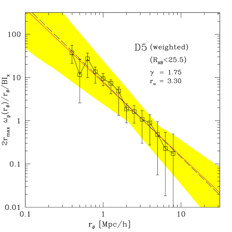
The results for the $\sigma_{\rm DLA}$-weighted CCF is shown in Figure 2. We find best-fitting parameters of ($r_{0}\,[h^{-1}{\rm\,Mpc}],\gamma)=(3.37\pm 0.36,1.77\pm 0.21)$ and $(3.43\pm 0.06,1.66\pm 0.03)$ for the D5 and G5 runs, respectively, as shown by the blue long-dashed line (see also Table 2). (See Section 5.1 for the error estimates.) Both results show good agreement with the best-fitting values of Cooke et al. (2006b, $r_{0}=3.32\pm 1.25$ and $\gamma=1.74\pm 0.36$). The result of D5 is somewhat noisy at $r\lesssim 1\,h^{-1}{\rm\,Mpc}$, which originates from the noisy pair-count of $N_{i}D_{\rm DLA}D_{\rm LBG}$.

The parameter values given in Table 2 clearly show that the $\sigma_{\rm DLA}$-weighted method gives larger values of $r_{0}$ and a slightly steeper power-law slope. In a CDM universe, the number of low-mass haloes is far greater than that of massive haloes. Therefore, even a small weighting by $N_{i}$ boosts up the overall pair-count, yielding a stronger correlation signal compared to the unweighted case. The larger LBG sample in the G5 run makes its result more robust against the weighting procedure than that of the D5 run. Therefore, the difference in the slope $\gamma$ between the two calculation methods is smaller in the G5 run than that of D5 run.

5.1 Confidence Limits

The $\chi^{2}$ test describes the goodness-of-fit of the model to the data. To determine the confidence intervals of the two parameters ($\gamma$ and $r_{0}$), we use the minimum $\chi^{2}$ method. This statistic is written as

$$\chi^{2}\equiv\sum_{i=1}^{n}\frac{(O_{i}-E_{i})^{2}}{\sigma_{i}^{2}},$$ (5)

where $O_{i}$ are the data points shown in the correlation figures, $E_{i}$ are the expected values in each bin $i$ from the power-law, and $\sigma_{i}$ is the standard deviations in each bin obtained from the 100 Monte Carlo calculations, as described earlier.

The region of confidence limits (Avni, 1976) is given by

$$\chi^{2}_{p}=\chi^{2}_{\rm min}+\Delta(df,p),$$ (6)

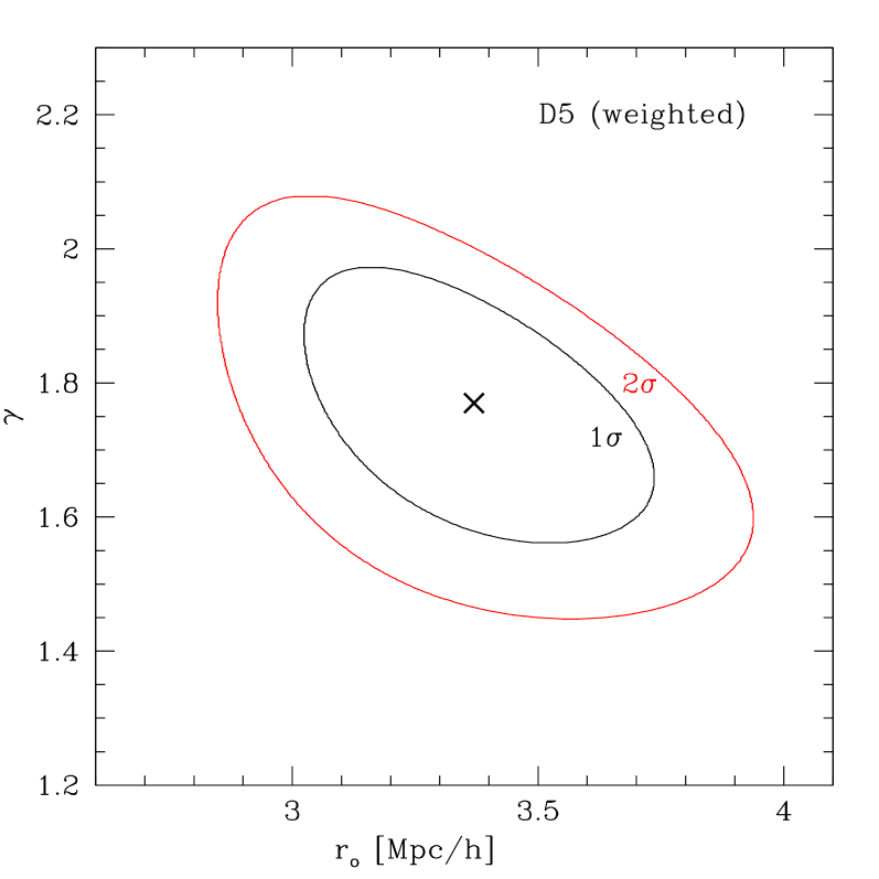
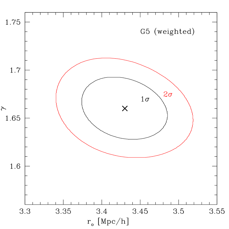
where $p$ is a confidence level ($0<p<1$), and $df$ is a degree of freedom written as $df=n-c$, where $n$ is the number of bins and $c$ is the number of parameters. For this work, $c=2$ and $n=13$ for G5 DLA-LBG CCFs (un-weighted and $\sigma_{DLA}$-weighted), G5 LBG-LBG ACF, and G5 DLA-DLA ACFs (un-weighted and $\sigma_{DLA}$-weighted); $n=14$ for D5 DLA-LBG 3D and $angular$ CCFs (un-weighted and $\sigma_{DLA}$-weighted); and $n=17$ for G5 DLA-LBG $angular$ CCFs (un-weighted and $\sigma_{DLA}$-weighted). The value $\Delta(df,p)$ is the expected increment of $\chi^{2}$ to find the 68$\%$ and 95$\%$ confidence limits above $\chi^{2}_{\rm min}$. Its value is determined by the degree of freedom and probability within 1 and 2-$\sigma$ limits. We calculate the 1-$\sigma$ confidence limits for all the correlation cases using this method. As an example, we show the 1 and 2-$\sigma$ confidence levels for the weighted CCFs of D5 and G5 runs in Figure 3.

Figure 3: Two parameter confidence limit contours for the weighted DLA-LBG cross correlation case using the minimum $\chi^{2}$ method. The best fits of the two parameters are indicated by the cross at the center of the contours, and 1 and 2-$\sigma$ limits are shown in black and red contour lines, respectively.

6 Angular cross correlation function

In observational studies, a different method is usually used to obtain the values of ($r_{0}$, $\gamma$) compared with what we described in Sections 4 and 5, because the precise estimation of any LBG position along the line of sight is difficult to achieve owing to redshift uncertainties caused by peculiar velocities and galactic winds. With such imprecision, it is not possible to measure the CCF at scales $r\lesssim 1h^{-1}{\rm\,Mpc}$ reliably. Therefore, rather than attempting to estimate the 3-D distance between DLAs and LBGs, observers usually employ the angular CCF using the projected data on the sky. For example, Cooke et al. (2006a, b) computed the angular CCF using the method proposed by Adelberger et al. (2003). In order to compare our results with those by Cooke et al’s, we briefly describe the calculation method of Adelberger et al. (2003), and then describe how we perform our measurement of the angular CCF.

With a power-law assumption, the expected number of pairs for the projected angular CCF is

$$\omega_{p}(r_{\theta}<r_{z})=\frac{r_{0}^{\gamma}r_{\theta}^{1-\gamma}}{2r_{z}}B\left(\frac{1}{2},\frac{\gamma-1}{2}\right)I_{x}\left(\frac{1}{2},\frac{\gamma-1}{2}\right),$$ (7)

where $B$ and $I_{x}$ are the beta and incomplete beta functions with (e.g., Press et al., 1992)

$$x\equiv r_{z}^{2}\left(r_{z}^{2}+r_{\theta}^{2}\right)^{-1}.$$ (8)

Adelberger et al. (2003) proposed to count the number of pairs in cylindrical shells of angular separation $r_{\theta}\pm\delta r_{\theta}$ and redshift separation $r_{z}\pm\delta r_{z}$, rather than using spherical shells. By setting $r_{z}$ to

$$r_{z}={\rm max}\left(1000\,{\,\rm km\,s^{-1}}\frac{(1+z{x})}{H(z)},7r_{\theta}\right),$$ (9)

the lower limit ensures that the redshift errors do not lead to the underestimate of the number of pairs, and the upper limit allows sufficient distances to include enough correlated pairs (Adelberger et al., 2003).

For our calculations, we focus at $z=3$ and thus $r_{z}={\rm max}(12.8\,h^{-1}{\rm\,Mpc},7r_{\theta})$. With simple algebra, Equation (7) can be converted to a more familiar power-law form:

$$\xi(r_{\theta}) = 2r_{\rm max}\frac{\omega_{p}(r_{\theta})}{r_{\theta}}\biggl{[}B\left(\frac{1}{2},\frac{\gamma-1}{2}\right)I_{x}\left(\frac{1}{2},\frac{\gamma-1}{2}\right)\biggr{]}^{-1}$$ (10)

$$= \left(\frac{r_{\theta}}{r_{0}}\right)^{-\gamma},$$

where $r_{z}$ is set to $r_{\rm max}$. We change from spherical coordinates to cylindrical coordinates, and set the number of cylindrical bins to 20 in a logarithmic scale as before. All pair searches are extended to the adjacent box using periodic boundary conditions, if appropriate.

A few assumptions must be made while we deal with the beta and incomplete beta functions. There are two parameters ($\gamma$ and $x$) that must be given to calculate the values of $B$ and $I_{x}$. To calculate $\gamma$, we first plot Equation (10) without $B$ and $I_{x}$ (i.e., $2r_{\rm max}\omega_{p}(r_{\theta})/r_{\theta}$) and find the best-fitting value of $\gamma$. The value of $x$ is determined by $r_{z}$ and $r_{\theta}$ as shown in Equation (8). By setting $r_{z}=r_{\rm max}$, the angular separation will be divided into two different regimes. Within the smaller angular separation range ($100\,h^{-1}{\rm\,kpc}<r_{\theta}<1.83\,h^{-1}{\rm\,Mpc}$), the correlated pairs are counted up to the maximum radial distance of $r_{\rm max}=\pm 12.8\,h^{-1}{\rm\,Mpc}$ for a cylinder centred on an LBG or DLA, while in the larger separation range ($r_{\theta}>1.83\,h^{-1}{\rm\,Mpc}$) all the correlated pairs within $r_{\rm max}=\pm 7r_{\theta}$ are counted. We calculate the values of $B$ and $I_{x}$ (as well as the IC correction) separately for the two different $r_{\theta}$ regions. With the fixed values of $\gamma$ obtained above and 20 different values of $x$, $B$ and $I_{x}$ can be calculated for each bin.

Figure 4: DLA-LBG angular CCFs at $z=3$ computed by the unweighted method for the D5 and G5 runs. Other features are the same as described in Figure 1.

Figure 5: DLA-LBG angular CCFs at $z=3$ computed by the $\sigma_{\rm DLA}$-weighted method for the D5 and G5 runs. Other features are the same as described in Figure 1.

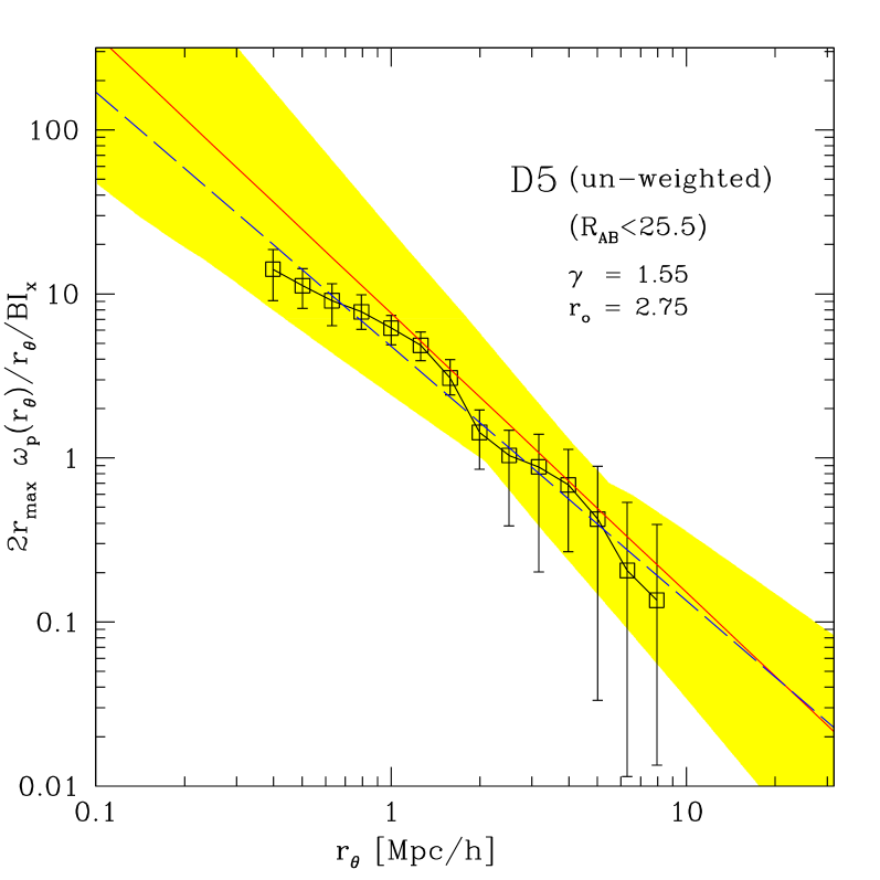
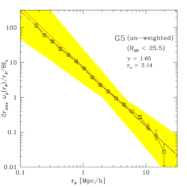
The angular CCF results of our calculations are shown in Figures 4 and 5 for both the unweighted and the $\sigma_{\rm DLA}$-weighted method. The best-fitting power-law parameters are given in Table 3. Again, the agreement with the results of Cooke et al. (2006a, b) is within a good range. Similarly to the 3-D CCF case, the $\sigma_{\rm DLA}$-weighted case gives a slightly larger $r_{0}$ and steeper $\gamma$ than the unweighted case. The unweighted case of D5 is shallow with $\gamma=1.55$, but in the $\sigma_{\rm DLA}$-weighted case, $\gamma\simeq 1.75$ is recovered.

	Unweighted		$\sigma_{\rm DLA}$-weighted
Run	$r_{0}$	$\gamma$	$r_{0}$	$\gamma$
D5	2.75 $\pm$ 0.51	1.55 $\pm$ 0.20	3.30 $\pm$ 0.60	1.75 $\pm$ 0.23
G5	3.14 $\pm$ 0.28	1.65 $\pm$ 0.09	3.42 $\pm$ 0.32	1.69 $\pm$ 0.10

Table 3: Best-fitting power-law parameters for the angular CCF at $z=3$. The units of the parameters are the same as in Table 2. The confidence limit statistics are described in Section 5.1. For comparison, Cooke et al. (2006b) reported $r_{0}=3.32\pm 1.25\,h^{-1}{\rm\,Mpc}$ and $\gamma=1.74\pm 0.36$ for their angular CCF.

7 Auto-correlation functions

7.1 LBG auto-correlation

The auto-correlation function (ACF) also gives important constraints on the distribution of the population under study. In this section, we calculate the 3-D LBG ACF by changing all subscripts in Equation (LABEL:eq:xi01) to ‘LBG’:

$$\xi_{\rm LBG-LBG}(r)={}$$

$${}\frac{D_{\rm LBG}D_{\rm LBG}-2D_{\rm LBG}R_{\rm LBG}+R_{\rm LBG}D_{\rm LBG}}{R_{\rm LBG}R_{\rm LBG}}{}.$$

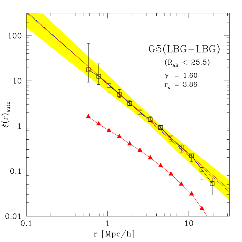
Our result for the ACF is shown in Figure 6, and the best-fitting power-law parameters (see Section 5.1 for confidence limit statistics) are $r_{0}=3.86\pm 0.13\,h^{-1}{\rm\,Mpc}$ and $\gamma=1.60\pm 0.07$. The last two data points were not included for the power-law fit because they are likely underestimated owing to the limited box-size. Our values of $r_{0}$ and $\gamma$ agree well with the observational estimates of Adelberger et al. (2003) and Adelberger et al. (2005), who measured the values of $r_{0}=4.0\pm 0.6\,h^{-1}{\rm\,Mpc}$ and $\gamma=1.57\pm 0.14$ for the LBG ACF at $z\sim 3$, with a correction for the integral constraint.

The dark matter ACF (the red filled triangles in Figure 6) was also computed as described in Nagamine et al. (2008) in order to calculate the bias of LBGs against the dark matter distribution (see Section 8).

Figure 6: LBG auto-correlation function at $z=3$ for the G5 run. The yellow shade shows the 1-$\sigma$ range of the best-fitting power-law of Adelberger et al. (2005). The variance of the ACF using 100 random seeds is shown with vertical errorbars. The red solid and blue dashed lines are the best-fitting power-laws of Adelberger et al. (2005) and this work, respectively. The last two data points were not included for the power-law fit. The red filled triangles show the dark matter ACF at the same redshift.

7.2 DLA auto-correlation

Similarly to the LBG ACF, it would be useful to compute the DLA ACF in order to estimate the DLA host halo mass. Observers also may be able to calculate the DLA ACF in the future when they accumulate a large enough sample of DLAs. In this section, we calculate the DLA ACF with both the unweighted and the $\sigma_{\rm DLA}$-weighted methods. By replacing all subscripts to ‘DLA’ in Equations (7.1) and (LABEL:eq:xi02), we obtain

$$\textstyle\xi_{\rm DLA-DLA}(r)={}$$

$${}\frac{\textstyle D_{\rm DLA}D_{\rm DLA}-2D_{\rm DLA}R_{\rm DLA}+R_{\rm DLA}R_{\rm\rm DLA}}{\textstyle R_{\rm DLA}R_{\rm DLA}}{}$$

and

$$\textstyle\xi_{\rm DLA-DLA}^{\rm weighted}(r)={}$$

$${}\frac{\scriptstyle N_{i}N_{j}D_{\rm DLA}^{i}D_{\rm DLA}^{j}-2N_{i}N_{j}D_{\rm DLA}^{i}R_{\rm DLA}^{j}+N_{i}N_{j}R_{\rm DLA}^{i}R_{\rm DLA}^{j}}{\scriptstyle N_{i}N_{j}R_{\rm DLA}^{i}R_{\rm DLA}^{j}},{}$$

where $N_{i}N_{j}D_{\rm DLA}^{i}D_{\rm DLA}^{j}$ and $N_{i}N_{j}D_{\rm DLA}^{i}R_{\rm DLA}^{j}$ are the numbers of data-data pairs and data-random pairs, weighted by the number of DLA pixels $N_{i}$ and $N_{j}$. As before, 100 different realisations of random dataset have been used to examine the statistical variance.

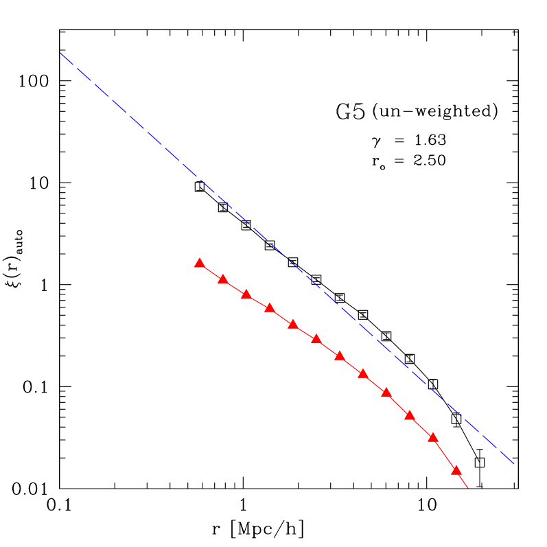
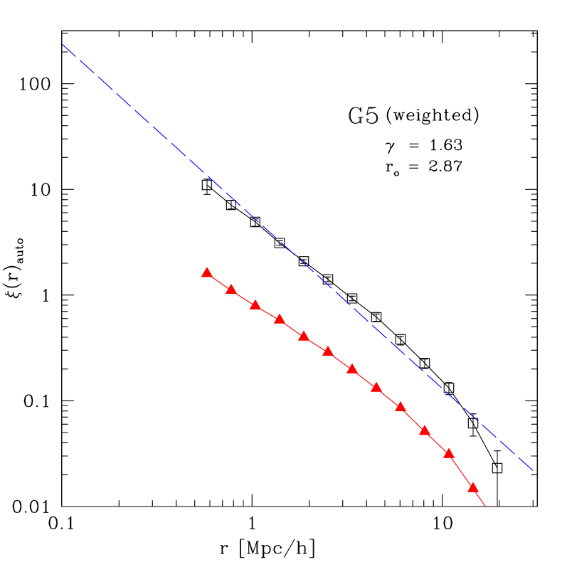
Our DLA ACF result is shown in Figure 7, and we find the best-fitting power-law parameters (see Section 5.1 for confidence limit statistics) of $r_{0}=2.50\pm 0.03\,h^{-1}{\rm\,Mpc}$ and $\gamma=1.63\pm 0.02$ for the unweighted ACF, and $r_{0}=2.87\pm 0.05\,h^{-1}{\rm\,Mpc}$ and $\gamma=1.63\pm 0.03$ for the $\sigma_{\rm DLA}$-weighted ACF, as summarised in Table 4. The values of $\gamma$ are similar to those for the LBG ACF with $\gamma\simeq 1.6$, but $r_{0}$ is much smaller. This is owing to the lower average DLA halo mass compared to the LBG host haloes, as we will discuss further in Section 8.

Figure 7: DLA auto-correlation function calculated with unweighted and $\sigma_{\rm DLA}$-weighted method for the G5 run. The variance of ACFs using 100 random seeds is shown with vertical errorbars. The blue dashed lines are best-fits for this work.

		$r_{0}$	$\gamma$
LBG-auto		3.86 $\pm$ 0.13	1.60 $\pm$ 0.07
DLA-auto (unweighted)		2.50 $\pm$ 0.03	1.63 $\pm$ 0.02
DLA-auto ($\sigma_{\rm DLA}$-weighted)		2.87 $\pm$ 0.05	1.63 $\pm$ 0.03

Table 4: ACFs of LBGs and DLAs for the G5 run. The results of unweighted and $\sigma_{\rm DLA}$-weighted methods are given for the DLA ACF. $r_{0}$ is in units of $h^{-1}{\rm\,Mpc}$. The confidence limit statistics are described in Section 5.1. For comparison, Adelberger et al. (2005) reported $r_{0}=4.0\pm 0.6\,h^{-1}{\rm\,Mpc}$ and $\gamma=1.57\pm 0.14$ for the LBGs at $z\simeq 3$.

8 Bias and Halo Masses

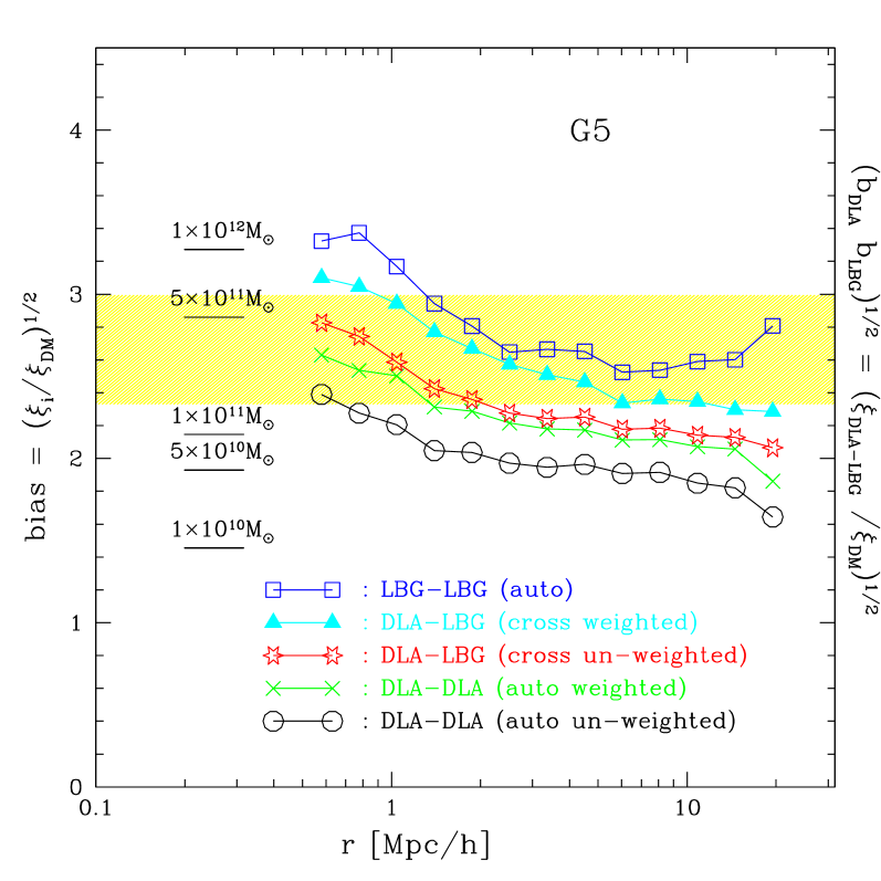
Comparing the correlation functions of DLAs and LBGs with that of dark matter gives the measure of ‘bias’ for the spatial distribution of these populations against that of dark matter. Each observation probes certain spatial scales, and one can compute the average bias and a corresponding average halo mass of the observed sample. In Figure 8, we show the bias of the simulated DLAs and LBGs, defined as $b\equiv\sqrt{\xi_{i}/\xi_{\rm DM}}$, as a function of distance $r$, where $i={\rm LBG}$ or ${\rm DLA}$. This definition is based on the linear bias model,

$$\xi_{i}(r)=b_{i}^{2}\,\xi_{\rm DM}(r).$$ (14)

The corresponding expression for the cross-correlation is (Gawiser et al., 2001)

$$\xi_{\rm DLA-LBG}(r)=b_{\rm DLA}\,b_{\rm LBG}\,\xi_{\rm DM}(r).$$ (15)

Therefore, the two lines for the CCF in Figure 8 are in fact showing $\sqrt{b_{\rm DLA}b_{\rm LBG}}$, as indicated on the axis on the right-hand-side. Taking the ratio of the above two expressions gives (Cooke et al., 2006b)

$$\frac{\xi_{\rm DLA-LBG}(r)}{\xi_{\rm LBG}}=\frac{b_{\rm DLA}}{b_{\rm LBG}}.$$ (16)

We also show the observed range of bias for the LBGs at $z=3$ by Adelberger et al. (2005) as a yellow shaded region. In all cases shown in Figure 8, the bias of simulated DLAs and LBGs slowly decreases with increasing distance. The upturn at $r=20\,h^{-1}{\rm\,Mpc}$ for the LBG ACF is probably just noise. We take a simple average of bias values across the logarithmic bins at $r=1.40-14.5\,h^{-1}{\rm\,Mpc}$, and find $\bar{b}=2.65$, $2.48$, $2.24$, $2.17$ and $1.94$ for LBG ACF, DLA-LBG CCF ($\sigma_{\rm DLA}$-weighted), DLA-LBG CCF (unweighted), DLA ACF ($\sigma_{\rm DLA}$-weighted), and DLA ACF (unweighted), respectively. The values of $r_{0}$ also reflect the sizes of average bias values. We took the above range of scales for taking the average because most of the recent observations are probing the scale of $r\simeq 1-10\,h^{-1}{\rm\,Mpc}$.

Gawiser et al. (2007) used the results of Adelberger et al. (2005) to obtain an average bias of $\bar{b}_{\rm LBG}=2.5\pm 0.4$ for LBGs at $z\sim 3$. Our average bias value of 2.60 for the LBG ACF is very close to that of Adelberger et al. (2005), and at the lower end of the estimate of $\bar{b}_{\rm LBG}=3.0\pm 0.5$ by Lee et al. (2006)

The model of Sheth & Tormen (1999) shows that an understanding of the unconditional mass function can provide an accurate estimation of the large-scale bias factor. From our average bias, we calculate the mean halo mass for LBGs and DLAs (using the unweighted and the $\sigma_{\rm DLA}$-weighted results) based on the method described in Mo & White (2002), as shown in Table 5. Our calculation of LBG halo mass is very close to that by Adelberger et al. (2005), $M_{\rm halo}^{\rm LBG}=10^{11.2}-10^{11.8}M_{\odot}$ (yellow shade in Fig. 8), which is very encouraging. Finally, Bouche et al. (2005) estimated $\langle\log M_{\rm DLA}\rangle=11.13\pm 0.13$ from observations and $\langle\log M_{\rm DLA}\rangle=11.16$ from simulations. These values are somewhat higher than the upper limit of our unweighted DLA halo mass and close to our $\sigma_{\rm DLA}$-weighted one. Cooke et al. (2006a) also obtained a similar value of $M_{\rm halo}\simeq 10^{11.2}M_{\odot}$.

Alternatively, we can directly calculate the mean DLA halo mass using the simulation result without going through the bias argument. For the G5 run, the mean is $\log\langle M_{\rm halo}^{\rm DLA}\rangle=11.5$ and $\langle\log M_{\rm halo}^{\rm DLA}\rangle=11.3$. These values are somewhat higher than the mean halo mass reported in Table 5. However, the values of $\langle M_{\rm halo}\rangle$ in Table 5 are computed from the average bias within the range of $r=1.40-14.5\,h^{-1}{\rm\,Mpc}$, and they could become higher if we included the bins at smaller scales. Since observers probe mostly $r\simeq 1-10\,h^{-1}{\rm\,Mpc}$, the values reported in Table 5 are more appropriate for comparison with observations.

Bouche & Lowenthal (2004) defined the parameter $\alpha$ as the ratio of correlation functions: $\alpha\equiv\overline{b}_{\rm CCF}(M_{\rm DLA})/\overline{b}_{\rm ACF}(M_{\rm LBG})$. If the value of $\alpha$ is larger (or smaller) than unity, then the mean halo mass of DLAs is more (or less) massive than that of the LBGs. The ratio of the average bias of LBG ACF and DLA-LBG CCF is $\alpha=0.727$ for our results. This value is in good agreement with the observational estimates of $\alpha=1.62\pm 1.32$ (Bouche & Lowenthal, 2004), $\alpha=0.73\pm 0.08$ (Bouche et al., 2005), and $\alpha=0.771$ (Bouche et al., 2005; Mo & White, 2002).

		$\overline{bias}$	$\log\langle M_{\rm halo}\rangle$
LBG-auto		$2.67^{+0.28}_{-0.06}$	$11.53^{+0.22}_{-0.06}$
DLA-auto (unweighted)		$1.94^{+0.11}_{-0.13}$	$10.71^{+0.16}_{-0.19}$
DLA-auto ($\sigma_{\rm DLA}$-weighted)		$2.17^{+0.14}_{-0.13}$	$11.02^{+0.14}_{-0.16}$

Table 5: Average biases and halo masses of LBGs and DLAs for the G5 run. The plus and minus values next to the average bias show the upper and lower limits at $1.40<r<14.5$ $h^{-1}{\rm\,Mpc}$. Mean halo masses are computed from the second column following Mo & White (2002) and given in units of $M_{\odot}$.

Figure 8: The biases of all correlation functions at $z=3$ that we computed in this paper for the G5 run. The tick marks on the left-hand-side show the host halo masses calculated with the method described in Mo & White (2002). The yellow shade shows the upper and lower limits by Adelberger et al. (2005).

9 Discussion and Conclusions

Our study represents a first attempt to calculate the DLA-LBG cross-correlation function at $z=3$ using cosmological SPH simulations. We calculated the DLA-LBG CCFs in several different approaches: 3-D, angular, unweighted, and $\sigma_{\rm DLA}$-weighted. We also computed the auto-CF of LBGs and DLAs, and the bias against dark matter. In comparison to the observational data by Adelberger et al. (2005); Cooke et al. (2006a, b), we find good agreement between our simulations and observational measurements. Our results suggest that the spatial distribution of DLAs and LBGs are strongly correlated.

Let us summarise some of the main conclusions of this work. In the first part of this paper, our results on the 3-D CCF calculated with spherical shells (Table 2) are to be compared with the 3-D spherical shell result by Cooke (private communication), $r_{0}=3.39\pm 1.2\,h^{-1}{\rm\,Mpc}$ and $\gamma=1.61\pm 0.3$. Our results are consistent with Cooke’s within the error. The shallow slope of Cooke’s above estimate probably owes to the limited sample size in the spherical shell at small distances, as we discussed in Sections 4 and 6.

In the second part, we have replaced the spherical shell method with the projected approach used in Adelberger et al. (2003) and Cooke et al. (2006b), and calculate the best-fitting values given in Table 3. Encouragingly, our results are within the upper and lower limits of the observational measurement by Cooke et al. (2006a, b). We corrected all CFs in this paper with the integral constraint.

Finally, we also analysed the auto-correlation functions of LBGs and DLAs at $z=3$ (Table 4) found in our simulations. Our results for the best-fitting parameters of the LBG ACF agree well with Adelberger et al. (2005). Our results show that LBGs are more strongly correlated than DLAs, and have higher mean halo mass.

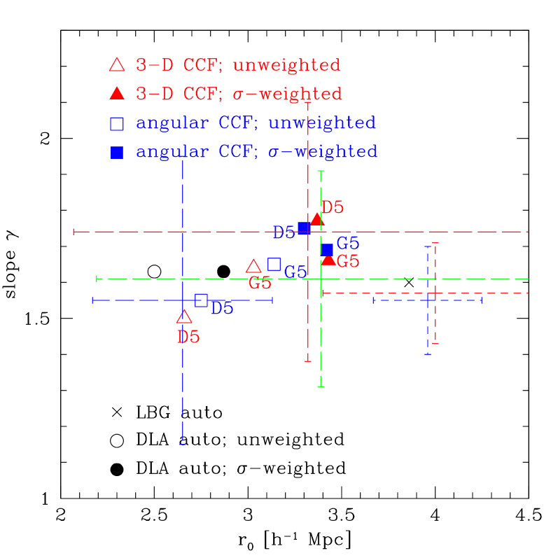
Figure 9 summarises the best-fitting power-law parameters for all the correlation functions that we obtained in the earlier sections. In most cases, the slope $\gamma$ falls into the range $\approx 1.5-1.7$ and the variation is not very large. The correlation length $r_{0}$ shows a larger variation from $2.5\,h^{-1}{\rm\,Mpc}$ to $4\,h^{-1}{\rm\,Mpc}$, depending on the sample and calculation method. This trend is similar to that seen by Cooke et al. (2006b, Fig. 8). In general, the $\sigma_{\rm DLA}$-weighted method gives a larger $r_{0}$ than the unweighted method.

Figure 9: Summary of best-fitting power-law parameters for all correlation functions that we obtained in earlier sections. Long blue, red, and green dashed cross lines are for the LBG ACF, the angular CCF, and the 3-D CCF of Cooke et al. (2006a, b), respectively. The LBG ACF of Adelberger et al. (2003) is shown in a short blue dashed line and of Adelberger et al. (2005) is shown in red.

Finally, the LBG bias, derived from the LBG ACF in Section 8, has led to the upper and lower limits of the LBG dark matter halo mass of $\log\langle M_{\rm halo}\rangle=11.53^{+0.22}_{-0.06}$ (see Table 5). This result is consistent with observational estimates of the LBG halo mass of $M_{\rm halo}\sim 10^{12}M_{\odot}$, (e.g., Steidel et al., 1998; Adelberger et al., 1998) and within the limit of $M_{\rm halo}=10^{11.2}-10^{11.8}M_{\odot}$ (Adelberger et al., 2005). Similarly, we derived the DLA biases, and obtained the mean DLA halo masses as shown in Table 5. Cooke et al. (2006a)’s measurement showed a DLA galaxy bias of $b_{\rm DLA}\sim 2.4$ and an average DLA halo mass of $M_{\rm halo}\sim 10^{11.2}M_{\odot}$. Our average DLA bias ($\overline{b}=1.94$ and $\overline{b}=2.17$ for un-weighted DLA ACF and weighted DLA ACF, respectively) and halo mass estimates ($\log\langle M_{\rm halo}^{\rm DLA}\rangle$=10.71 and 11.02 for un-weighted DLA ACF and weighted DLA ACF, respectively) are in good agreement with theirs. We also examined the ratio of bias values defined as $\alpha\equiv\overline{b}_{\rm CCF}/\overline{b}_{\rm ACF}$ (Bouche & Lowenthal, 2004), and found that our value of $\alpha=0.727$ agrees well with the observational estimates. This again shows that the mean halo mass of DLAs is less than that of the LBGs. The fact that $\langle M_{\rm halo}^{\rm LBG}\rangle$ is greater than $\langle M_{\rm halo}^{\rm DLA}\rangle$ is a natural outcome because the LBG sample is limited to the bright star-forming galaxies with $R_{\rm AB}<25$ and $M_{\star}\simeq 10^{10}-10^{11}M_{\odot}$, whereas the DLA H i   gas is present in numerous lower mass haloes below the LBG threshold.

Motivated by our earlier successes of our simulations to reproduce the physical properties of LBGs such as stellar mass, SFR, and colours (Nagamine et al., 2004), in this work we examined another observational method, i.e. DLA-LBG CCF, to further check the consistency between observations and simulations. We found good agreement between our results and observations. Furthermore, there are accumulated evidence that suggest high halo masses for LBGs (e.g., Mo & Fukugita, 1996; Adelberger et al., 1998; Baugh et al., 1998; Giavalisco et al., 1998; Steidel et al., 1998; Kauffmann et al., 1999; Mo et al., 1999; Katz et al., 1999; Papovich et al., 2001; Shapley et al., 2001). Therefore, the scenario that the majority of LBGs is merger-induced starburst systems associated with low-mass haloes (Lowenthal et al., 1997; Sawicki & Yee, 1998; Somerville et al., 2001; Weatherley & Warren, 2003) does not appear to be a favored model for LBGs.

In our simulations, we estimated the H i   column densities using a pixel size that is much larger than the typical quasar beam size, which is of the order of parsecs. This may have some impact on our estimates of ${N_{\rm HI}}$ and the corresponding statistics such as the H i   column density distribution function. For example, if the ISM is clumpy on smaller scales than our pixel size, there could be high-density neutral clouds below our resolution scale that are self-shielded and contain larger amounts of H i  . Unfortunately, owing to limitations in computational resources, it is not possible for us at the moment to run such a high-resolution cosmological simulation with the same box size as we have used in this paper. In future work, we will nevertheless attempt to check the dependence of our ${N_{\rm HI}}$ estimates on numerical resolution, and perform more rigorous resolution tests.

References

- Adelberger et al. (1998) Adelberger K. L., Steidel C. C., Giavalisco M., Dickinson M., et al. 1998, ApJ, 505, 18
- Adelberger et al. (2005) Adelberger K. L., Steidel C. C., Pettini M., Shapley A. E., et al. 2005, ApJ, 619, 697
- Adelberger et al. (2003) Adelberger K. L., Steidel C. C., Shapley A. E., Pettini M., 2003, ApJ, 584, 45
- Avni (1976) Avni, Y. 1976, ApJ, 210, 642
- Bardeen et al. (1986) Bardeen J. M., Bond J. R., Kaiser N., Szalay A. S., 1986, ApJ, 304, 15
- Baugh et al. (1998) Baugh C. M., Cole S., Frenk C. S., Lacey C. G., 1998, ApJ, 498, 504
- Bouche et al. (2005) Bouche N., Gardner J. P., Weinberg D. H., Davé R., Lowenthal J. D., 2005, ApJ, 628, 89
- Bouche & Lowenthal (2004) Bouche N., Lowenthal J. D., 2004, ApJ, 609, 513
- Bruzual & Charlot (1993) Bruzual, G. A. & Charlot, S., 1993, ApJ, 405, 538
- Cooke et al. (2006a) Cooke J., Wolfe A. M., Gawiser E., Prochaska J. X., 2006a, ApJL, 636, L9
- Cooke et al. (2006b) Cooke J., Wolfe A. M., Gawiser E., Prochaska J. X., 2006b, ApJ, 652, 994
- Davé et al. (1999) Davé R., Hernquist L., Katz N., Weinberg D. H., 1999, ApJ, 511, 521
- Gawiser et al. (2007) Gawiser E., Francke H., Lai K., Schawinski K., et al., 2007, ApJ, 671, 278
- Gawiser et al. (2001) Gawiser E., Wolfe A. M., Prochaska J. X., Lanzetta K. M., et al. 2001, ApJ, 562, 628
- Giavalisco et al. (1998) Giavalisco M., Steidel C. C., Adelberger K. L., Dickinson M. E., et al. 1998, ApJ, 503, 543
- Haardt & Madau (1996) Haardt F., Madau P., 1996, ApJ, 461, 20
- Hernquist et al. (1996) Hernquist L., Katz N., Weinberg D. H., Miralda-Escude, J. 1996, ApJ, 457, L51
- Kaiser (1984) Kaiser N., 1984, ApJL, 284, L9
- Katz et al. (1999) Katz N., Hernquist L., Weinberg D. H., 1999, ApJ, 523, 463
- Katz et al. (1996) Katz N., Weinberg D. H., Hernquist L., 1996, ApJS, 105, 19
- Katz et al. (1996a) Katz N., Weinberg D. H., Hernquist L., Miralda-Escude, J. 1996, ApJ, 457, L57
- Kauffmann et al. (1999) Kauffmann G., Colberg J. M., Diaferio A., White S. D. M., 1999, MNRAS, 303, 188
- Landy & Szalay (1993) Landy S. D., Szalay A. S., 1993, ApJ, 412, 64
- Lee et al. (2006) Lee K.-S., Giavalisco M., Gnedin O. Y., Somerville R. S., et al. 2006, ApJ, 642, 63
- Lowenthal et al. (1997) Lowenthal J. D., Koo D. C., Guzman R., Gallego J., et al. 1997, ApJ, 481, 673
- Mo & Fukugita (1996) Mo H. J., Fukugita M., 1996, ApJ, 467, L9
- Mo et al. (1999) Mo H. J., Mao S., White S. D. M., 1999, MNRAS, 304, 175
- Mo & White (2002) Mo H. J., White S. D. M., 2002, MNRAS, 336, 112
- Nagamine et al. (2010) Nagamine K., Choi J.-H., Yajima H., 2010, ArXiv e-prints, 1006.5345
- Nagamine et al. (2008) Nagamine K., Ouchi M., Springel V., Hernquist L., 2008, ArXiv e-prints, 802
- Nagamine et al. (2004a) Nagamine K., Springel V., Hernquist L., 2004a, MNRAS, 348, 421
- Nagamine et al. (2004b) Nagamine K., Springel V., Hernquist L., 2004b, MNRAS, 348, 435
- Nagamine et al. (2004) Nagamine K., Springel V., Hernquist L., Machacek M., 2004, MNRAS, 350, 385
- Nagamine et al. (2007) Nagamine K., Wolfe A. M., Hernquist L., Springel V., 2007, ApJ, 660, 945
- Papovich et al. (2001) Papovich C., Dickinson M., Ferguson H. C., 2001, ApJ, 559, 620
- Peebles (1980) Peebles P. J. E., 1980, The large-scale structure of the universe. Research supported by the National Science Foundation. Princeton, N.J., Princeton University Press, 1980. 435 p.
- Pontzen et al. (2008) Pontzen A., Governato F., Pettini M., Booth C. M., et al. 2008, MNRAS, 390, 1349
- Press et al. (1992) Press W. H., Teukolsky S. A., Vetterling W. T., Flannery B. P., 1992, Numerical recipes in C. The art of scientific computing. Cambridge: University Press, —c1992, 2nd ed.
- Sawicki & Yee (1998) Sawicki M. J., Yee H. K. C., 1998, AJ, 115, 1329
- Shapley et al. (2001) Shapley A. E., Steidel C. C., Adelberger K. L., Dickinson M., et al. 2001, ApJ, 562, 95
- Sheth & Tormen (1999) Sheth R. K., Tormen G., 1999, MNRAS, 308, 119
- Somerville et al. (2001) Somerville R. S., Primack J. R., Faber S. M., 2001, MNRAS, 320, 504
- Springel (2005) Springel V., 2005, MNRAS, 364, 1105
- Springel & Hernquist (2002) Springel V., Hernquist L., 2002, MNRAS, 333, 649
- Springel & Hernquist (2003a) Springel V., Hernquist L., 2003a, MNRAS, 339, 289
- Springel & Hernquist (2003b) Springel V., Hernquist L., 2003b, MNRAS, 339, 312
- Springel et al. (2001) Springel V., White S. D. M., Tormen G., Kauffmann G., 2001, MNRAS, 328, 726
- Steidel et al. (1998) Steidel C. C., Adelberger K. L., Dickinson M., Giavalisco M., et al. 1998, ApJ, 492, 428
- Steidel et al. (1999) Steidel C. C., Adelberger K. L., Giavalisco M., Dickinson M., et al. 1999, ApJ, 519, 1
- Storrie-Lombardi & Wolfe (2000) Storrie-Lombardi L. J., Wolfe A. M., 2000, ApJ, 543, 552
- Weatherley & Warren (2003) Weatherley S. J., Warren S. J., 2003, MNRAS, 345, L29
- Wolfe et al. (2003) Wolfe A. M., Prochaska J. X., Gawiser E., 2003, ApJ, 593, 215
- Wolfe et al. (1986) Wolfe A. M., Turnshek D. A., Smith H. E., Cohen R. D., 1986, ApJS, 61, 249