Paired states in spin-imbalanced atomic Fermi gases in one dimension

Abstract

A growing expertise to engineer, manipulate and probe different cold-atom analogs of electronic condensed matter systems allows to probe properties of exotic pairing. We study paired states of spin-imbalanced ultracold atomic system of fermions with attractive short-range interactions in one-dimensional traps. Calculations are done using the Bethe Ansatz technique and the trap is incorporated into the solution via a local density approximation. The thermodynamic-Bethe-Ansatz equations are solved numerically and different local density profiles are calculated for zero and finite temperatures. A procedure to identify the homogeneous-system phase diagram using local density profiles in the trap is also proposed. Such scheme would be immediately useful for the experiments.

Recently, ultracold-atom realizations of condensed-matter-physics models have attracted a lot of interest. A growing expertise in engineering, tuning and probing atomic systems allows to study exceedingly complicated systems. One of the current challenges of condensed matter physics is to understand the different exotic paired states that are realized when paired particles have different chemical potentials. This disparity could be due to different physical effects such as different masses of the pairing particles or external magnetic filed and is thought to arise in systems such as quasi one-dimensional and two-dimensional organic superconductors Singleton et al. (2000) and heavy-fermion materials Radovan et al. (2003) to name a few. It is argued that the zero-center-of-mass-momentum Cooper pairs are destabilized due the population imbalance and different, unconventional, paired states are proposed to occur Sarma (1963); Liu and Wilczek (2003). Among these exotic states, the FFLO (Fulde-Ferrell-Larkin-Ovchinnikov) state, in which pairs have nonzero center-of-mass momentum and superconductivity (superfluidity) coexists with nonzero polarization, is one of the candidates Fulde and Ferrell (1964); Larkin and Ovchinnikov (1965). Recently, several experiments have studied the interplay of pairing and polarization in tree-dimensional (3d) spin-imbalanced superfluid clouds Zwierlein et al. (2006); Partridge et al. (2006). Ongoing experiments are exploring different pairing mechanisms in spin-imbalanced ultracold atomic systems of fermions in reduced dimensions Hul , where the FFLO state is believed to have a large parameter regime of stability. The ultracold cloud of atoms is subjected to a 2d optical lattice, which defines an array of quasi-1d tubes, which can be regarded as independent if the intensity of the laser beams is large enough to suppress tunneling among them. Thus, to explore pairing properties of 1d systems of spin-imbalanced fermions is very relevant. There have been many different recent studies of this system. Bosonization Yang (2001); Zhao and Liu (2008), Bethe Ansatz Orso (2007); Hu et al. (2007); Guan et al. (2007), mean field Liu et al. (2007), QMC Batrouni et al. (2008); Casula et al. (2008) and DMRG Feiguin and Heidrich-Meisner (2007); Rizzi et al. (2008); Tezuka and Ueda (2008); Feiguin and Huse (2008) methods have been used to study this problem and the agreement is that the partially polarized superfluid region (or “phase”) is the analog of the FFLO state in higher dimensions (see Fig. 1, explained below). Most of the past analysis was done for zero temperature, except the QMC and mean field calculations. In addition, these approaches find the regime of strong interactions between particles very challenging, while experiments are done preferably in that regime. Therefore, there is a need for finite-temperature calculations, which do not suffer of the above limitations.

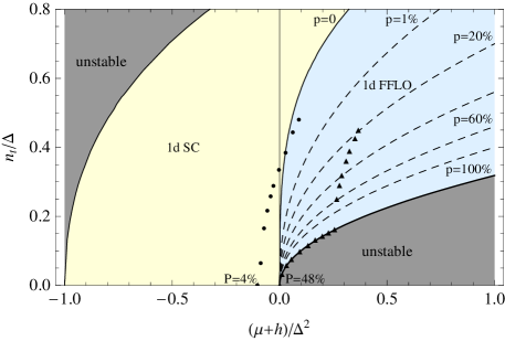
Figure 1: Zero-temperature phase digram of the uniform 1d system, showing BCS-like (1d SC), FFLO-like (1d FFLO) and (fully polarized) normal ($p=100\%$ curve) “phases”. The areas marked “unstable” correspond to parameter regimes, which do not support equilibrium states. Local density trap profiles for total polarizations $P=4\%$ (circles) and $P=48\%$ (triangles) are superimposed on the diagram.

In this paper, we address the problem using the Thermodynamic-Bethe-Ansatz (TBA) equations Takahashi (1970, 1971), which provide a full finite-$T$ description and are well posed for arbitrary interaction strengths. We also propose a scheme to reconstruct the “phase diagram” of a homogeneous 1d attractive fermion cloud from experimental profiles of local particle density and polarization in a trap. We start from the Hamiltonian of a single 1d tube in a harmonic trap

$$H=-\frac{\hbar^{2}}{2m}\sum_{i}\frac{\partial^{2}}{\partial z_{i}^{2}}+g_{\text{1D}}\sum_{i<j}\delta(z_{i}-z_{j})+\frac{m\omega_{z}^{2}}{2}\sum_{i}z_{i}^{2},$$ (1)

where $m$ is the mass of the atoms, $\omega_{z}$ is the trap frequency and $g_{\text{1D}}=\frac{2\hbar^{2}a_{\text{3D}}}{ma_{\perp}^{2}}\frac{1}{1-Ca_{\text{3D}}/a_{\perp}}$ [with $C=|\zeta(1/2)|/\sqrt{2}\simeq 1.0326$] is the effective interaction strength between particles, which can be tuned using a Feshbach resonance and made attractive ($g_{\text{1D}}<0$) Olshanii (1998). $a_{\text{3D}}$ is the 3d scattering length and $a_{\perp}$ is the transverse oscillator length. In what follows, we shall measure lengths in units of the harmonic oscillator length $(\hbar/m\omega_{z})^{1/2}$ and energies in units of $\hbar\omega_{z}/2$. The dimensionless Hamiltonian reads

$$H=-\sum\frac{\partial^{2}}{\partial z_{i}^{2}}-4\Delta\sum\delta(z_{i}-z_{j})+\sum z_{i}^{2},$$ (2)

where $\Delta=-\frac{g_{\text{1D}}}{2\hbar\omega_{z}}\sqrt{\frac{m\omega_{z}}{\hbar}}>0$ (attractive interactions). We will use the solution of the uniform system and take trap effects into account via the local density (Thomas-Fermi) approximation. This approximation is widely used in studying trapped gases, but its violation has been observed in highly elongated 3d clouds Partridge et al. (2006) due to interface interaction effects De Silva and Mueller (2006); Imambekov et al. (2006). In 1d, one rather finds smooth crossovers and, for attractive fermions, comparison with QMC calculations Casula et al. (2008) indicate that the local density approximation gives good results for density profiles. Most features of local trap profiles are faithfully reproduced, but for the short wavelength Friedel oscillations, which are washed out at finite temperatures. In this framework, the Bethe Ansatz solution of the model Yang (1967); Gaudin (1967) can be used locally. Eigenvalues and eigenstates of the system (of size $L$ and with periodic boundary conditions) are determined from the roots of the Bethe-Ansatz equations:

$$e^{ik_{j}L} = \prod_{m=1}^{M}\frac{k_{j}-\Lambda_{m}-i\Delta}{k_{j}-\Lambda_{m}+i\Delta},$$

$$-\prod_{m=1}^{M}\frac{\Lambda_{n}-\Lambda_{m}-2i\Delta}{\Lambda_{n}-\Lambda_{m}+2i\Delta} = \prod_{j=1}^{N}\frac{\Lambda_{n}-k_{j}-i\Delta}{\Lambda_{n}-k_{j}+i\Delta},$$

where $j=1,...,N$ and $n=1,...,M$ ($M\leq N/2$), with $N$ the total number of particles and $M$ the number of minority ones. $\{k_{i}\}$ are particle quasi-momenta and solely determine energy eigenvalues, $E=\sum_{j=1}^{N}k_{j}^{2}\equiv eL$. $\{\Lambda_{n}\}$ are (effective) spin rapidities and determine magnetic properties of the system. Analyzing the roots of the Bethe Ansatz equations one can find that there are three classes of solutions Takahashi (1971): real $k_{j}$-s, representing unpaired particles; bound states of two particles with opposite spins, represented by complex $k_{j}=\Lambda_{j}\pm i\Delta$, with real spin rapidity $\Lambda_{j}$; and complex spin rapidities forming strings $\Lambda^{(r)j}=\Lambda^{(r)}+i\Delta(r+1-2j)$, with $j=1,...,r$ and with real $\Lambda^{(r)}$ the center of the $r$-string.

In the thermodynamic limit, $L\rightarrow\infty$ (keeping $N/L$ and $M/L$ constant), it is possible to locally define root and hole density distributions for unpaired particles, bound states and $n$-strings: $\rho_{u}^{r(h)}(k,z)$, $\rho_{b}^{r(h)}(k,z)$ and $\rho_{sn}^{r(h)}(\Lambda,z)$. The partition function is defined as $Z=\text{Tr}e^{-H/T}=e^{-F/T}$, where $\frac{F}{L}={\cal F}(z)=e(z)-Ts(z)-\mu(z)n_{t}(z)-hn_{s}(z)$ is the free energy density, $\mu(z)=\mu_{0}-z^{2}$ is the local chemical potential, $h$ is the applied magnetic field, and $s(z)$, $n_{t}(z)$ and $n_{s}(z)$ are local entropy, total-particle and spin densities, respectively. Then the equilibrium root and hole density distributions are locally determined by minimizing the free energy while taking into account the Bethe-Ansatz equations. The resulting TBA equations Takahashi (1970, 1971) are

$$f_{u}-\bar{f}_{u}=G*f_{b}-G*f_{s1},$$

$$f_{b}-\bar{f}_{b}=2[k^{2}-\Delta^{2}-\mu(z)]/T+K_{1}*\bar{f}_{u}+K_{2}*\bar{f}_{b},$$

$$f_{sn}-\bar{f}_{sn}=\delta_{n,1}G*\bar{f}_{u}+G*(f_{sn+1}+\hat{\delta}_{n,1}f_{sn-1}),$$

$$\lim_{n\rightarrow\infty}(K{}_{n+1}*f_{sn}-K{}_{n}*f_{sn+1})=-2h/T,$$

where $f_{\alpha}=\ln(1+\rho_{\alpha}^{h}/\rho_{\alpha}^{r})$ and $\bar{f}_{\alpha}=\ln(1+\rho_{\alpha}^{r}/\rho_{\alpha}^{h})$ are functions related to probability distributions, $K_{n}(k)=\frac{1}{\pi}\frac{n\Delta}{k^{2}+(n\Delta)^{2}}$, $G(k)=\frac{1}{4\Delta\cosh\frac{\pi k}{2\Delta}}$ and ‘$*$’ indicates the convolution of two functions (these notations are as in Ref. Bolech and Andrei (2005)). In terms of the $f$’s, ${\cal F}(z)$ reads

$${\cal F}(z)=-\frac{T}{2\pi}\int dk\bar{f}_{u}(k,z)-\frac{T}{\pi}\int dk\bar{f}_{b}(k,z).$$ (3)

It is possible to straightforwardly determine densities of different thermodynamic variables from the free energy using $x(z)=-\frac{\partial{\cal F}(z)}{\partial\bar{x}(z)}$, where $x=n_{t},n_{s},s$ and $\bar{x}=\mu,h,T$ are conjugate thermodynamic variables. One can write equations for the different density distributions of all extensive thermodynamic variables in a compact form

$$\rho_{u}^{x,h}+\rho_{u}^{x,r}=G*\rho_{b}^{x,h}+G*\rho_{s1}^{x,h},$$ (4)

$$\rho_{b}^{x,h}+\rho_{b}^{x,r}=\delta_{x,n_{t}}/\pi-K_{1}*\rho_{u}^{x,r}-K_{2}*\rho_{b}^{x,r},$$

$$\rho_{sm}^{x,h}+\rho_{sm}^{x,r}=\delta_{m,1}G*\rho_{u}^{x,r}+G*(\rho_{sm+1}^{x,h}+\hat{\delta}_{m,1}\rho_{sm-1}^{x,h}),$$

$$\lim_{m\rightarrow\infty}(K{}_{n+1}*\rho_{sm}^{x,h}-K{}_{n}*\rho_{sm+1}^{x,h})=-\delta_{x,n_{s}}/\pi,$$

where the corresponding density distributions are defined as $\rho_{y}^{x,r}=(-1)^{\delta_{y,s}}\frac{1}{2\pi}\partial_{\bar{x}}(T\bar{f}_{y})$ and $\rho_{y}^{x,h}=(-1)^{1+\delta_{y,s}}\frac{1}{2\pi}\partial_{\bar{x}}(Tf_{y})$. Notice that the above system of equations for the particle density ($x=n_{t}$) coincides with the continuum limit of the Bethe-Ansatz equations. Using these definitions, local densities of thermodynamic observables in the trap are given by

$$x(z)=\int dk\rho_{u}^{x,r}(k,z)+2\int dk\rho_{b}^{x,r}(k,z).$$ (5)

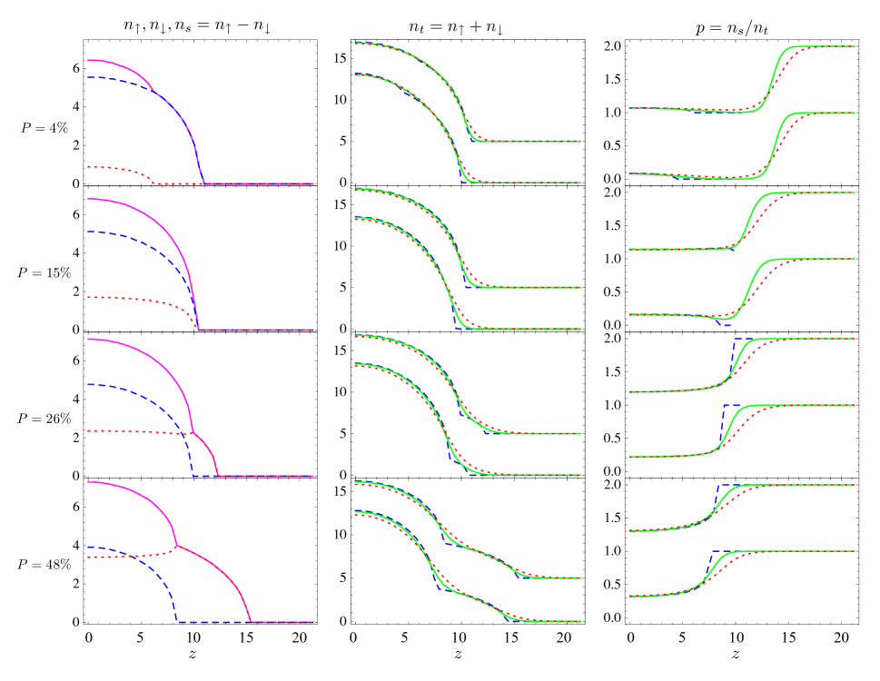
Figure 2: Trap density profiles for $N=200$, $T=0,0.06,0.12[\mu_{\uparrow F}]$ (dashed, solid and dotted, respectively) and different total polarization $P$. The first column shows spin-up ($n_{\uparrow}$, solid), spin-down ($n_{\downarrow}$, dashed) particle densities and their difference ($n_{s}$, dotted) for $\Delta=25$ and $T=0$ only. The second column shows the local particle densities ($n_{t}$) for $\Delta=25,100$ and different temperatures. The third column shows the respective local polarizations ($p$). The $n_{t}$ and $p$ plots for $\Delta=25$ are vertically offset for clarity.

The integral equations are solved numerically for different temperatures and interaction strengths (cf. Ref. Bolech and Andrei (2005)); different density profiles are plotted in Fig. 2. The reference chemical potential, $\mu_{0}$, and the magnetic field, $h$, are fixed by the self-consistency relations $\int dz\,n_{t}(z)=N$ and $\int dz\,n_{s}(z)=PN$. Depending on $P$, trap profiles show different regimes that reveal properties of the zero-temperature “phase digram” of a uniform system. For small polarizations ($P=4\%$ plots), an FFLO-like state in the trap center coexists with a BCS-like state at the edges; while for large polarizations ($P=26\%$ and $P=48\%$ plots), the FFLO-like state in the trap center coexists with a fully polarized normal state at the edges. Close to the “critical point” ($P=15\%$ plots), the entire trap is in the FFLO-like state. The interface between different “phases” in the trap is marked by a kink feature in the local particle density (or polarization) profiles at zero temperature, which is smeared out by thermal fluctuations. From Fig. 2 we see that while for cases with large total polarization the phase boundary is still visible at $T=0.06\,[\mu_{\uparrow F}]$ (here $\mu_{\uparrow F}$ is the noninteracting Fermi energy for the majority species), for small polarizations temperature should be even smaller to observe the kink. From the local polarization profiles, we see that in the normal state temperature induces bound pairs, while in the fully paired state unpaired particles appear.

We propose here a scheme to identify the low-temperature “phase diagram” of the uniform system from trap profiles of the local particle density and polarization. To achieve that aim we represent the phase diagram in variables that can be measured directly in the experiments. We argue that $n_{t}(z)$ and the majority-spin local chemical potential $\mu_{\uparrow}(z)=\mu(z)+h$ can be straightforwardly measured and, thus, a “phase diagram” in these variables should be directly useful to analyze experimental findings. In these variables, the “phase diagram” of the uniform system (see Fig. 1) shows three different states: the BCS-like fully paired state with zero polarization (1dSC), the FFLO-like state with non-zero polarization (1dFFLO) and the fully polarized normal state which has collapsed into a curve (cf. Fig. 1 in Ref. Orso (2007)). Plotting the local particle density and polarization profiles as functions of $\mu_{\uparrow}$ will reconstruct the uniform-system “phase diagram” and probe into the 1dFFLO state. To elucidate the scheme we consider a trap profile with the total polarization $P=48\%$ (triangles on Fig. 1). In this regime, the 1dFFLO “phase” in the trap center coexists with the fully polarized region at the edges (see Fig. 2). In the framework of the local density approximation, the radius of the cloud is given by $R=\sqrt{\mu_{0}+h}$ and thus one can easily find $\mu_{\uparrow}(z)+h=R^{2}-z^{2}$. Thus, the trap profile can be uniquely placed on the “phase digram” (see Fig. 1). The above identification is valid for clouds with fully polarized wings and plotting many profiles of these type allows to probe into the 1dFFLO. For small total polarizations, the 1dFFLO in the trap center coexists with the 1dSC regions at the edges (see Fig. 2). In this case, the radius of the cloud is given by $R=\sqrt{\Delta^{2}+\mu_{0}}$ and thus one can easily find $\mu_{\uparrow}(z)+h=R^{2}+h-\Delta^{2}-z^{2}$. It is again possible to place a trap profile on the “phase digram” (see trap profile for $P=4\%$ in Fig. 1). Due to the nonzero temperature and measurement noise, it will be challenging to precisely identify the zero polarization curve (1dFFLO-1dSC boundary), but most features of the “phase diagram” (including inner 1dFFLO isopolarization lines) are, nevertheless, within the reach of the upcoming experiments.

To summarize, we have studied different pairing states in spin-imbalanced ultracold atomic clouds of fermions in 1d. We have combined the Bethe Ansatz method and the local density approximation to calculate trap profiles of different observables. Our full finite-temperature calculations shed light on the parameter regimes for total density, polarization and temperature that are required to observe exotic states such as the 1dFFLO. We also proposed a way to unambiguously reconstruct the “phase” diagram of the uniform system from experimental local density profiles of the trapped clouds. Our calculational scheme could also be used to compute asymptotic momentum distributions that could be measured after simultaneously releasing the trap and switching off the interactions in time-of-flight experiments. This would be complementary to the in-situ pair-momentum correlators discussed already in the literature Batrouni et al. (2008); Casula et al. (2008); Feiguin and Heidrich-Meisner (2007); Rizzi et al. (2008); Tezuka and Ueda (2008) which are deemed to provide extra signatures of FFLO physics. A similar analysis can be also performed for repulsive interactions between particles, where the coexistence of different Luttinger-liquid regimes has been proposed Kakashvili et al. (2008). The above approach is well suited to explore interesting crossover effects, which are challenging to capture with other methods. Such a system would also be within the reach of the present generation of experiments.