Equilibria in the secular, non-coplanar two-planet problem

Abstract

We investigate the secular dynamics of a planetary system composed of the parent star and two massive planets in mutually inclined orbits. The dynamics are investigated in wide ranges of semi-major axes ratios (0.1–0.667), and planetary masses ratios (0.25–2) as well as in the whole permitted ranges of the energy and total angular momentum. The secular model is constructed by semi-analytic averaging of the three-body system. We focus on equilibria of the secular Hamiltonian (periodic solutions of the full system), and we analyze their stability. We attempt to classify families of these solutions in terms of the angular momentum integral. We identified new equilibria, yet unknown in the literature. Our results are general and may be applied to a wide class of three-body systems, including configurations with a star and brown dwarfs and sub-stellar objects. We also describe some technical aspects of the semi-numerical averaging. The HD 12661 planetary system is investigated as an example configuration.

1 Introduction

Nowadays, about thirty extrasolar multi-planet systems have been detected. Many of them seem either locked in or close to low-order mean motion resonances (MMRs). Moreover, there is a class of the so called hierarchical systems (Lee & Peale, 2003) which can be characterized by relatively small ratio of semi-major axes. Their planetary orbits are well separated and far from collision zones, hence the long-term, qualitative dynamics of such systems may be effectively investigated with secular theories. The Hamiltonian of a hierarchical system can be averaged out over mean longitudes which play the role of fast angles. In the regime of small eccentricities and inclinations, this approach leads to the well known, classical Laplace-Lagrange (L-L) secular theory (Murray & Dermott, 2000). It relies on the expansions of the disturbing function in power series with respect to eccentricities and inclinations which are small parameters of the problem. However, many multi-planet hierarchical systems do not satisfy the assumption of small eccentricities, and the L-L theory may fail.

Still, to deal with the observed diversity of orbital configurations, the secular theories relying on high-order expansions of the perturbations are used, e.g., the series in eccentricity (e.g., Murray & Dermott, 2000; Rodríguez & Gallardo, 2005; Libert & Henrard, 2006, 2007a, 2007b; Veras & Armitage, 2007) or expansion to the third order in the ratio of semi-major axes $\alpha$, known as the octuple theory (Ford et al., 2000; Lee & Peale, 2003). This theory can be also generalized to higher orders (Migaszewski & Goździewski, 2008, and references therein). The analytical expansions are particularly suitable for studies of hierarchical systems. Moreover, they are usually valid only in limited ranges of the orbital parameters, and special cases (like resonant configurations) must be treated individually. The alternative, recently developed quasi-analytical theory relies on averaging the perturbing Hamiltonian numerically (Michtchenko & Malhotra, 2004; Michtchenko et al., 2006). In this work, we are heavily inspired by these papers and their idea of the semi-analytical technique. Because the method does not require any expansion of the perturbing Hamiltonian, basically, it has no limitations inherent in the analytical theory. For instance, with a help of this technique, Michtchenko & Malhotra (2004) found new, non-classic feature of the secular dynamics of coplanar system of two planets (the so called non-linear secular resonance in the regime of large eccentricity). In the later work, Michtchenko et al. (2006) consider more general three-dimensional (3-D) secular model of two-planet system, and present a systematic approach helpful to investigate the global dynamics of such configurations.

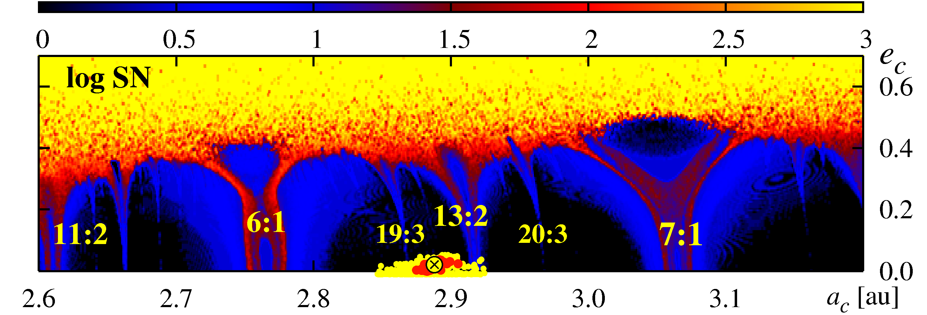
Figure 1: The dynamical map of the edge-on, coplanar HD 12661 system in the $(a_{\mbox{\scriptsize c}},e_{\mbox{\scriptsize c}})$-plane, for the best-fit solution to the RV data published in (Butler et al., 2006). Large values of the Spectral Number (SN) marked in yellow indicate continuous spectrum of the fundamental frequencies of the system and strongly chaotic motions, small SN (black) means discrete frequencies and ordered motions. Positions of low-order MMRs are labeled. The best-fit solution, yielding $(\chi^{2}_{\nu})^{1/2}\sim 1.08$ and an rms $\sim 7.46$ ms^-1, in terms of parameter tuples ($m$ [$\mbox{m}_{\mbox{\scriptsize J}}$], $a$ [au], e, $\omega$ [deg], ${\cal M}$ [deg]) including planetary mass, semi-major axis, eccentricity, the argument of pericenter and the mean anomaly at the epoch of the first observation, $t_{0}$=JD2,450,831.608380, is the following (2.34, 0.831, 0.361, 296.24, 126.86) for planet b, and (1.84, 2.888, 0.021, 52.66, 66.18) for planet c, respectively. The original errors are rescaled by adding stellar jitter of $3.5$ m/s in quadrature. The mass of the parent star is 1.11 $M_{\sun}$. Solutions within $1\sigma$ level of the best fit are marked with yellow circles, fits with marginally worse $(\chi^{2}_{\nu})^{1/2}$ are marked in red.

As an example to study, we choose the HD 12661 planetary system (Fischer et al., 2001; Fischer et al., 2003; Butler et al., 2006). The discovery paper (Fischer et al., 2001) announces two Jovian planets on well separated orbits with semi-major axes of $\sim 0.8$ au and $\sim 2.8$ au, respectively, and of moderate eccentricities. We analyzed the most recent, publicly available data from the catalogue of Butler et al. (2006) and (Wright et al., 2008), using the $N$-body model of the radial velocities (RV) and the so called hybrid minimization (Goździewski & Migaszewski, 2006). The results of our analysis of the RV data published in (Butler et al., 2006) are illustrated in Fig. 1. The best fit solution yielding $(\chi^{2}_{\nu})^{1/2}\sim 1.08$ and an rms $\sim 7.5$ m/s is marked with a crossed circle in the dynamical map in terms of the Spectral Number (SN) (Michtchenko & Ferraz-Mello, 2001). The SN is the fast indicator making it possible to distinguish between chaotic and regular planetary configurations. The osculating elements of the best fit solution at the epoch of the first observation are given in caption to Fig. 1. In this figure, we mark the semi-major axis and eccentricity of the outer planet derived from an ensemble of fits within $1\sigma$ of the best fit solution. Clearly, the available data already constrain orbital elements of the outer planet very well. The dynamical maps reveal orbits well separated from the low-order MMRs. Two most prominent MMRs within the vicinity of the best fit are 19:3 and 13:2 MMRs, respectively. Moreover, the best-fits within $1\sigma$ confidence level span the region of small eccentricities in which the resonances are very narrow.

Hence, the HD 12661 system fits well assumptions of the secular theory. This system has been studied already in a few papers: with the direct numerical integrations (Ji et al., 2003), with the analytical octupole theory of hierarchical systems (Lee & Peale, 2003), with mapping of the phase space by fast indicators (Goździewski, 2003a), and with the classic analytical theory that relies on expansions of the perturbation in eccentricity (Rodríguez & Gallardo, 2005; Libert & Henrard, 2006). All the cited works assume that the HD 12661 system is coplanar and oriented edge-on. However, we should keep in mind that a major limitation of the Doppler technique lies in the ambiguity of orbital inclinations, which cannot be well determined by far. The observational windows are still relatively narrow, and to remove the inclination degeneracy, several orbital periods of the outermost orbit are required. Moreover, the recent formation theories do not fully predict mutual inclinations in multi-planet systems. We cannot be certain yet whether the common assumption of coplanar orbits really holds true. Likely, many different forming scenarios are possible. For instance, the migration in low-order MMRs may end up with systems characterized by large mutual inclinations (Thommes & Lissauer, 2003). The dynamical relaxation of initially dense planetary systems of giant planets (Adams & Laughlin, 2003) may lead to scattering events which produce wide distribution of the mutual inclinations. Indeed, recent simulations of Veras & Ford (2008) revealed that the outer planet of the HD 12661 system undergoes large oscillations for nearly all of the allowed two-planet orbital solutions. These authors conclude that it might be the effect of a perturbation of planet c, perhaps due to strong scattering of an additional planet that was subsequently accreted onto the star. Moreover, we stress that the inclination of the HD 12661 system is still unknown, hence the understanding of basic features of its 3-D dynamics seems also important. This intriguing system is an excellent candidate for tests and numerical experiments regarding non-coplanar configurations. Moreover, because we attempt to study the secular 3-D dynamics globally, our results are general and valid for much wider class of three-body systems. The secular theory which we consider here, covers planetary systems with different masses and semi-major axes ratios, and the full range of mutual inclinations.

The plan of this work is the following. In Sect. 2, we recall the general mathematical model of the 3-D two-planet system. Subsection 2.1 is devoted to a short technical overview of the averaging approach and some computational details that may be useful in a practical implementation of the method. To make the paper self-contained, we also recall the notion of representative planes, and energy levels calculated for fixed values of the total angular momentum integral (Sect. 3). To illustrate the precision of the semi-analytic approach, we compute the Poincaré cross sections, and demonstrate chaotic behavior of the secular system (Michtchenko et al., 2006). The main results are described in Sect. 4 which is devoted to the analysis of the existence and bifurcations of equilibria in the secular, spatial problem of two mutually interacting planets. In particular, we detect and investigate closely a few families of these equilibria in a wide range of planetary mass ratio, $\mu\in\{0.25,0.5,1,2\}$, and the semi-major axes ratio, $\alpha\in\{0.1,0.2,0.333,0.667\}$. The results are general and valid as long as the partition of the Hamiltonian onto the Keplerian, integrable term, and the small perturbation is reasonable. In that part, our work extends the paper of Libert & Henrard (2007b). After introducing non-singular canonical variables, they investigate the existence, stability and bifurcations of stationary solutions emerging from the equilibrium at zero-eccentricities, the so called Lidov–Kozai resonance (Lidov, 1961; Kozai, 1962; Lidov & Ziglin, 1976; Thomas & Morbidelli, 1996; Innanen et al., 1997; Kinoshita & Nakai, 2007, to mention a few papers in an endless list of references) which was found and intensively investigated in the restricted three body problem. The full three-body problem in the Hill case (hierarchical configurations) was also intensively studied by many authors (e.g., Krasinsky, 1972, 1974; Lidov & Ziglin, 1976; Ferrer & Osacar, 1994; Miller & Hamilton, 2002; Fabrycky & Tremaine, 2007). These works rely mostly on the second order expansion of the secular Hamiltonian in the semi-major axes ratio (the quadrupole approximation). In the present work, we focus on two aspects of the problem:

• we consider the unrestricted problem in wide ranges of semi-major axes ratio $\alpha$, up to 0.667, and mass ratio $\mu$,

• we study equilibria of the full secular Hamiltonian; the semi-analytic averaging helps us to compute the secular perturbations beyond convergence limits of the usual power series expansions.

Thanks to the quasi-analytic averaging, we found new families of equilibria of the secular 3D planetary problem which unlikely may be detected with the help of perturbation techniques. We also study the Lyapunov stability of these solutions in detail (or to an extent permitted by technical limits of the semi-analytic algorithm).

2 The 3-D dynamics of two-planet system

The Hamiltonian of the three-body planetary system, expressed with respect to canonical Poincaré variables (see Laskar & Robutel, 1995; Michtchenko et al., 2006) has the form of:

$$\mathcal{H}=\underbrace{\sum_{i=1}^{2}{\bigg{(}\frac{1}{2\beta^{*}_{i}}\mathbf{p}_{i}^{2}-\frac{\mu^{*}_{i}\beta^{*}_{i}}{r_{i}}\bigg{)}}}_{\textrm{\small Keplerian part}}-\underbrace{\frac{k^{2}m_{1}m_{2}}{\Delta}}_{\textrm{\small direct part}}+\underbrace{\frac{\mathbf{p}_{1}\cdot\mathbf{p}_{2}}{m_{0}}}_{\textrm{\small indirect part}},$$ (1)

where ${\mathbf{r}_{i}}$ denote the position vectors relative to the star, ${\mathbf{p}_{i}}$ – their conjugate momenta relative to the barycenter of the full three-body system, ${\Delta=|\mathbf{r}_{1}-\mathbf{r}_{2}|}$ is for the distance between planets, ${m_{0}}$ – is the mass of the parent star; ${m_{1}}$, ${m_{2}}$ – are for the masses of the planets (also index $i=1$ is for the inner planet, and $i=2$ for the outer planet). We denote also the mass parameters ${\mu^{*}_{i}=k^{2}~{}(m_{0}+m_{i})}$ and the reduced masses through ${\beta^{*}_{i}=(1/m_{i}+1/m_{0})^{-1}}$. Under the assumption of $m_{i}\ll m_{0}$ (or, more generally, for small enough perturbations of Keplerian orbits), the Hamiltonian of the system, ${\cal H}$, is a sum of the Keplerian term (which would be integrable in the absence of mutual interactions between planets) and the interaction term with the so called direct and indirect terms.

Alternatively, the dynamical state of the system, $({\mathbf{r}_{i}},{\mathbf{p}_{i}})$ may be represented through the mass-weighted canonical angle–action variables of Delaunay (Murray & Dermott, 2000):

$$\begin{array}[]{ll}{\cal M}_{i}-\textrm{the mean anomaly},&{L_{i}=\beta^{*}_{i}~{}\sqrt{\mu^{*}_{i}~{}a_{i}}},\\ {\omega_{i}}-\textrm{the argument of pericenter},&{G_{i}=L_{i}~{}\sqrt{1-e_{i}^{2}}},\\ {\Omega_{i}}-\textrm{the longitude of node},&{H_{i}=G_{i}\cos~{}I_{i},}\end{array}$$ (2)

where $a_{i}$ denote semi-major axes, $e_{i}$ – eccentricities, and $I_{i}$ stand for inclinations; $(L_{i},G_{i},H_{i})$ are the conjugate momenta. The transformation between $({\mathbf{r}_{i}},{\mathbf{p}_{i}})$ and the set of Delaunay elements $(a_{i},e_{i},I_{i},\Omega_{i},\omega_{i},{\cal M}_{i})$ may be found in (Ferraz-Mello et al., 2005) or (Morbidelli, 2002). If orbits are far from strong MMRs and collision zones then Hamiltonian in Eq. 1 can be averaged out with respect to the mean anomalies playing the role of fast angles, and then we obtain the secular Hamiltonian ${\cal H_{\mbox{\scriptsize sec}}}$ which approximates the long-term, slow variations of the mean elements.

To make the paper self-contained, we recall basic facts on the secular 3-D problem of two planets. We follow Michtchenko et al. (2006) and Libert & Henrard (2007b). The averaged $\mathcal{H}_{sec}$ does not depend on ${\cal M}_{1},{\cal M}_{2}$, therefore the conjugate actions $(L_{1},L_{2})$ are constant. After the partial reduction of nodes, ${\cal H}_{\mbox{\scriptsize sec}}$ depends on $\Delta{\Omega}$ only, and not on $\Omega_{1}$ and $\Omega_{2}$ separately. After the canonical transformation (Michtchenko et al., 2006):

$$\begin{array}[]{l}(\omega_{1},G_{1})\\ (\omega_{2},G_{2})\\ (\Omega_{1},H_{1})\\ (\Omega_{2},H_{2})\end{array}\quad\Rightarrow\quad\begin{array}[]{l}(\omega_{1},G_{1})\\ (\omega_{2},G_{2})\\ \left(\theta_{1}=\frac{1}{2}\left(\Omega_{1}+\Omega_{2}\right),\ J_{1}=H_{1}+H_{2}\right)\\ \left(\theta_{2}=\frac{1}{2}\left(\Omega_{1}-\Omega_{2}\right),\ J_{2}=H_{1}-H_{2}\right).\end{array}$$ (3)

The secular Hamiltonian does not depend on $\theta_{1}$, therefore $J_{1}=|\mathbf{C}|=\mbox{const}$, where $\mathbf{C}$ is the total angular momentum of the system. Moreover, $\theta_{2}=\pi/2=\mbox{const}$ (in the Laplace frame, $2\theta_{2}\equiv\Delta\Omega=\pm\pi$, after Jacobi’s elimination of the nodes), and:

$$J_{2}=(G_{1}^{2}-G_{2}^{2})/J_{1}.$$

For fixed angular momentum $J_{1}$ and secular energy ${\cal H}_{\mbox{\scriptsize sec}}$, the averaged system can be reduced to two degrees of freedom. Instead of $J_{1}$, we may use the so called Angular Momentum Deficit, $\mathrm{AMD}=L_{1}+L_{2}-J_{1}.$ The $\mathrm{AMD}$ is a measure of the system non-linearity (Laskar, 2000). Coplanar and circular orbits have the minimum of $\mathrm{AMD}=0$. In configurations with large $\mathrm{AMD}$, crossing orbits are possible and they are very unstable.

Because the secular Hamiltonian still depends on many parameters, the global analysis of the long-term dynamics are complex. To simplify the study of their basic properties, we fix particular values of integrals and/or orbital elements. We choose the semi-major axes and masses as the primary parameters of the secular model. Then $L_{1}$ and $L_{2}$ are their (scaled) representation. The maximum of $\mathrm{AMD}$ is equal to $L_{1}+L_{2}$, hence we introduce the normalized Angular Momentum Deficit:

$${\mathcal{\cal A}}=\frac{\mathrm{AMD}}{L_{1}+L_{2}},\quad{\mathcal{\cal A}}\in[0,1],$$

which is an uniform and non-dimensional representation of $\mathrm{AMD}$. Relative to the Laplace plane, $C_{x}=C_{y}=0$, $C_{z}\equiv C$, hence we have:

$$L_{1}\sqrt{1-e_{1}^{2}}\cos I_{1}+L_{2}\sqrt{1-e_{2}^{2}}\cos I_{2}=J_{1},$$

$$L_{1}\sqrt{1-e_{1}^{2}}\sin I_{1}-L_{2}\sqrt{1-e_{2}^{2}}\sin I_{2}=0.$$

Also the mutual inclination of orbits ${{\cal I}_{\mbox{\scriptsize mut}}}=I_{1}+I_{2}$. Thus, $\cos{{\cal I}_{\mbox{\scriptsize mut}}}=\cos I_{1}\cos I_{2}+\sin I_{1}\sin I_{2}\cos\Delta\Omega$, or, alternatively,

$$\cos{{\cal I}_{\mbox{\scriptsize mut}}}(e_{1},e_{2}) = \frac{J_{1}^{2}-G_{1}^{2}-G_{2}^{2}}{2G_{1}G_{2}},$$ (4)

$$\cos I_{1}(e_{1},e_{2}) = \frac{J_{1}^{2}+G_{1}^{2}-G_{2}^{2}}{2J_{1}G_{1}},$$ (5)

$$\cos I_{2}(e_{1},e_{2}) = \frac{J_{1}^{2}+G_{2}^{2}-G_{1}^{2}}{2J_{1}G_{2}}.$$ (6)

Because $C\equiv C_{z}>0$, the above relations are singular for $I_{1}=I_{2}=\pi/2$ or $e_{1}=e_{2}=1$ (when $G_{1}=G_{2}=0$). A boundary of the manifold of permitted motions for a given $J_{1}\equiv C$ (or $\mathrm{AMD}$), semi-major axes and planetary masses ratio, can be defined through ${{\cal I}_{\mbox{\scriptsize mut}}}=0,\pi$. It can be also shown that when $\mathrm{AMD}$ is fixed and $I_{1,2}<\pi/2$ then the mutual inclination at the origin $(e_{1}=0,e_{2}=0)$ is maximal. We will denote such value by $i_{0}$ from hereafter.

The dynamics of the secular system are expressed through solutions to the following canonical equations of motion:

$$\frac{\mbox{d}\omega_{i}}{\mbox{d}t}=\frac{\partial{{\cal H}_{\mbox{\scriptsize sec}}}}{\partial{G_{i}}},\quad\frac{\mbox{d}G_{i}}{\mbox{d}t}=-\frac{\partial{{\cal H}_{\mbox{\scriptsize sec}}}}{\partial{\omega_{i}}},\quad i=1,2,$$ (7)

where $(\omega_{1},\omega_{2})$ are canonical angles and $(G_{1},G_{2})$ are canonical momenta. Having only the numerical approximation of ${\cal H}_{\mbox{\scriptsize sec}}$ (see below), we must solve Eqs. 7 numerically. For that purpose, we may use a suitable integrator, for instance, the 4-th order Runge-Kutta scheme (Press et al., 1992). The partial derivatives appearing in the right-hand side of the equations of motion, are calculated with the mid-point rule (Press et al., 1992). Moreover, to calculate precisely the Hessian of ${\cal H}_{\mbox{\scriptsize sec}}$ which is required to determine the stability (see Sect. 3.2), we are forced to use higher order approximations of the second order partial derivatives.

2.1 The semi-analytical averaging

The problem is now to average out the Hamiltonian, Eq. 1. We calculate:

$$\mathcal{H}_{sec}=\frac{1}{(2\pi)^{2}}~{}\int_{0}^{2\pi}\int_{0}^{2\pi}{\mathcal{H}~{}d{\cal M}_{1}~{}d{\cal M}_{2}}\equiv\left<{\cal H}\right>,$$ (8)

where ${\cal H}$ is the Hamiltonian of the problem expressed through the canonical Delaunay elements. For small enough perturbations, the Keplerian part of $\left<{\cal H}\right>$ depends on constant $L_{i}$ only and does not affect the secular evolution of the system. It can be shown that the average of the indirect part of Hamiltonian equals to a constant (Brouwer & Clemence, 1961). In the non-resonant case, we have to average out the direct part of disturbing Hamiltonian only.

The analytical calculation of apparently trivial integral, Eq. 8, is in fact a difficult problem. Usually, the Hamiltonian is expanded in power series with respect to appropriate small parameter (eccentricity, inclination or semi-major axes ratio). Then with the help of a suitable canonical transformation, we can “remove” particular terms of the Hamiltonian. However, the secular series converge for relatively small values of parameters. Instead, as we mentioned already, the secular Hamiltonian, Eq. 8, can be computed numerically, without troublesome power series expansions. This bright idea of Michtchenko & Malhotra (2004) is quite simple to apply.

Apparently, to compute integral in Eq. 8, we must evaluate $\mathcal{H}$ in a discrete grid of the mean anomalies. That would imply multiple (and in fact unnecessary) solution of the Kepler equation. To get rid of this problem, we can change the variables under the double integral using the well known expressions relating the mean $({\cal M}_{i})$, true ($f_{i}$) and eccentric (${\cal E}_{i}$) anomalies, respectively.

      

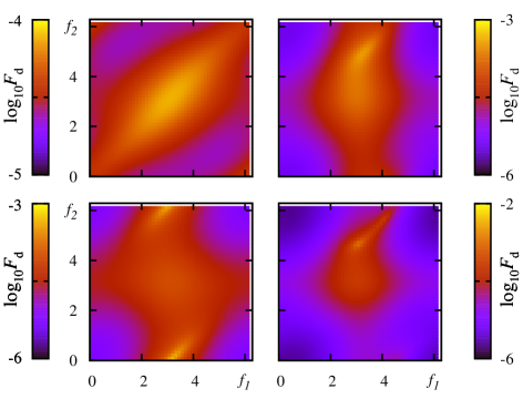
Figure 2: The left-hand panels are for contour levels of function $(\mathcal{F}_{\mbox{\scriptsize d}}$ in the $(f_{1},f_{2})$–plane, computed for the coplanar two-planet system and orbital parameters: $m_{0}=1~{}M_{\odot}$, $m_{1}=1~{}\mbox{m}_{\mbox{\scriptsize J}}$, $m_{2}=3~{}\mbox{m}_{\mbox{\scriptsize J}}$, $a_{1}=1$ au, $a_{2}=3$ au. Eccentricities and $\Delta{\varpi}$ are different at each panel: the top left-hand panel is for $e_{1}=0.1$, $e_{2}=0.2$, $\Delta{\varpi}=0$, the top right-hand panel is for $e_{1}=0.6$, $e_{2}=0.5$, $\Delta{\varpi}=\pi/2$, the bottom left-hand panel is for $e_{1}=0.4$, $e_{2}=0.5$, $\Delta{\varpi}=\pi$, the bottom right-hand panel is for $e_{1}=0.6$, $e_{2}=0.7$, $\Delta{\varpi}=\pi/2$. Panels in the right-hand column illustrate the AMR-like division of the integration domain, as depending on the variability of the integrand function.

To express the double integral through the true anomalies, we differentiate the Kepler equation ${\cal M}_{i}={\cal E}_{i}-e_{i}\sin{{\cal E}_{i}}$, with respect to ${\cal M}_{i},{\cal E}_{i}$, and then we find that $d\,{\cal M}_{i}={\cal J}_{i}~{}\mbox{d}\,f_{i}$, where:

$${\cal J}_{i}\equiv{\cal J}_{i}(e_{i},f_{i})=\left(1-e_{i}^{2}\right)^{3/2}~{}\left(1+e_{i}\cos{f_{i}}\right)^{-2},\quad i=1,2.$$ (9)

The secular Hamiltonian has the following form:

$$\mathcal{H}_{sec}=\frac{1}{(2\pi)^{2}}~{}\int_{0}^{2\pi}\int_{0}^{2\pi}{{\cal F}~{}df_{1}~{}df_{2}},\quad{\cal F}={\cal H}{\cal J}_{1}{\cal J}_{2}.$$ (10)

We may also express the double integral through eccentric anomalies that leads to even simpler expressions for functions ${\cal J}_{i}$. Next, to calculate the integral in Eq. 10, we apply an adaptive-grid integration algorithm that relies on the Gauss-Legendré quadrature of the 64-th order. The adaptive algorithm is forced by large variability of the integrand function. To illustrate that issue, we analyse a few typical examples shown in Fig. 2. The left-hand contour plots in this figure are for the shape of direct term of ${\cal H}$ (Eq. 1) multiplied by ${\cal J}_{1}{\cal J}_{2}$, ${\cal F}_{\mbox{\scriptsize d}}$, in the $(f_{1},f_{2})$-plane. These plots are computed for different values of eccentricities and $\Delta{\varpi}=\varpi_{1}-\varpi_{2}$, where $\varpi_{1,2}$ are the longitudes of periastron. In this experiment, the system is coplanar. In the top-left panel of Fig. 2 (see its left-hand part), which corresponds to relatively small eccentricities, ${\cal F}_{\mbox{\scriptsize d}}$ is weakly varying function of $(f_{1},f_{2})$. But for large eccentricities, it may have narrow extrema in some parts of the $(f_{1},f_{2})$-plane (see the bottom-right contour plot in Fig. 2). In these areas, to reach a desired accuracy, the integral must be computed on a dense grid of the $(f_{1},f_{2})$-plane. However, in other parts of the grid, such a large number of quadrature nodes is not necessary and, under the requirement of fixed accuracy, it would cause significant CPU overhead. Thus, the optimal computation of the double integral is possible with the non-uniform grid in the $(f_{1},f_{2})$-plane, following an idea of adaptive quadratures [see, for instance, Press et al. (1992)]. In the right-hand part of Fig. 2, we illustrate the steps of our simple adaptive mesh integration by appropriate divisions of the integration subintervals. Typically, the number of divisions is small but in some parts of the $(f_{1},f_{2})$-plane, it may be as large as 8–9, in order to obtain the relative error of $\epsilon\sim 10^{-12}$ in two subsequent steps of the integration.

3 Equilibria in the 3-D secular problem

According to the classic methodology of Poincaré, to understand the dynamics, one should investigate whole families of solutions. Isolated orbits in the phase space tell us little on the global properties of the system. The most simple class of solutions that can be investigated efficiently in any two degree of freedom Hamiltonian system are equilibria defined through algebraic equations:

$$\frac{\mbox{d}\omega_{i}}{\mbox{d}t}=0,\quad\frac{\mbox{d}G_{i}}{\mbox{d}t}=0,\quad i=1,2.$$ (11)

Typically, one tries to find the phase-space coordinates of these equilibria, their number and bifurcations as well as to determine their Lyapunov stability (at least, the linear stability). The analysis of the existence and bifurcations of equilibria in the secular 3D system are quite complex because they depend on many parameters ($\mathrm{AMD}$, the total energy, particular orbital elements, masses of planetary companions). Hence, to investigate such solutions globally, we have to choose a proper representation of the phase space regarding these parameters. Moreover, to avoid limitations of the analytical approach, the whole analysis should be done numerically, by the semi-analytical averaging. Hence, a reduction of the dimension of the phase space is critically important.

3.1 The representative planes of the energy

To simplify the search for equilibria of ${\cal H}_{\mbox{\scriptsize sec}}$, we choose a specific two-dimensional plane of initial conditions that makes it possible to represent the stationary solutions in the 4-D phase-space of the secular system. We follow Michtchenko et al. (2006) and Libert & Henrard (2007b). The representative plane of initial conditions (the $\cal S$-plane from hereafter) should have common points with each phase trajectory of the secular system. In Michtchenko et al. (2006), the $\cal S$-plane is defined through:

$${\cal P}_{M}=\{e_{1}\cos{\Delta{\varpi}}\times e_{2}\cos{2\omega_{1}}\},$$

where $e_{1,2}\in[0,1]$ and angles $(\Delta{\varpi},2\omega_{1})$ are fixed to pairs of angles $(0,0)$, $(\pi,0)$, $(0,\pi)$, and $(\pi,\pi)$, respectively. In that notion, the $\cal S$-plane comprises of four subsets of points which coordinates span the range of $e_{1}\cos\Delta\varpi\in[-1,1]$ and $e_{2}\cos 2\omega_{1}\in[-1,1]$.

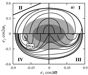
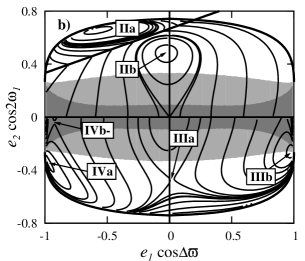
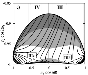
Figure 3: Generic plots of ${\cal H}_{\mbox{\scriptsize sec}}$ in the ${\cal P}_{M}$-plane of $(e_{1}\cos{\Delta\varpi},~{}e_{2}\cos{2\omega_{1}})$ obtained for $\alpha=0.333$, $\mu=0.5$ and ${\mathcal{\cal A}}=0.10$ (a) and ${\mathcal{\cal A}}=0.25$ (b) and ${\mathcal{\cal A}}=0.85$ (c), respectively. Small Roman numbers label families of stationary solutions identified in this work (see the text for more details). Solid thick line marks the collision line of orbits defined through $a_{1}(1\mp e_{1})=a_{2}(1-e_{2})$. Shaded regions mark mutual inclinations. Panel (a) $[0^{\circ},50^{\circ}]$ (white), $[50^{\circ},60^{\circ}]$ (light gray), and $\geq 60^{\circ}$ (dark gray), respectively. The limit values of inclinations for panel (b) are, $0^{\circ}$, $95^{\circ}$ and $105^{\circ}$, respectively; for panel (c): $0^{\circ}$, $140^{\circ}$ and $155^{\circ}$.

Subsequent panels of Fig. 3 show generic views of the ${\cal P}_{M}$-plane derived for different values of ${\mathcal{\cal A}}$ integral and the same primary parameters, ($\alpha,\mu$). In particular, these plots are drawn for ${\cal H}_{\mbox{\scriptsize sec}}$ levels which are found numerically as solutions to ${\cal H}_{sec}-E_{0}=0$, where $E_{0}$ is a fixed value, for the following values of the semi-major axes and masses ratios: $\alpha=a_{1}/a_{2}=0.333$, $\mu=m_{1}/m_{2}=0.5$, and ${\mathcal{\cal A}}=0.10$ (the left-hand panel), ${\mathcal{\cal A}}=0.25$ (the middle panel), and ${\mathcal{\cal A}}=0.85$ (the right-hand panel), respectively. According with the general construction of the $\cal S$-plane, it is divided by four quadrants and, for a reference, labeled with Roman numbers in the left-hand panel of Fig. 3: quadrant I ($\Delta\varpi=0$, $\omega_{1}=0$), quadrant II ($\Delta\varpi=\pi$, $\omega_{1}=0$), quadrant III ($\Delta\varpi=0$, $\omega_{1}=\pi/2$), and quadrant IV ($\Delta\varpi=\pi$, $\omega_{1}=\pi/2$).

Alternatively, we also use another definition of the $\cal S$-plane:

$${\cal P}_{S}=\{e_{1}\sin{\omega_{1}}\times e_{2}\sin{\omega_{2}}:\omega_{1},\omega_{2}=\pm\pi/2;e_{1,2}\in[0,1)\},$$ (12)

(see Libert & Henrard, 2007b). The ${\cal P}_{S}$-plane helps to avoid a discontinuity of the levels of ${\cal H}_{\mbox{\scriptsize sec}}$ at the $x$-axis. In fact, that plane carries out the same information as the negative ($y<0$) part of the ${\cal P}_{M}$-plane. Obviously, pairs of angles of the ${\cal P}_{S}$ representation: ($\omega_{1}=+\pi/2,\omega_{2}=-\pi/2$), ($\omega_{1}=+\pi/2,\omega_{2}=+\pi/2$), ($\omega_{1}=-\pi/2,\omega_{2}=-\pi/2$), ($\omega_{1}=-\pi/2,\omega_{2}=+\pi/2$), correspond to the following pairs of angles in the ${\cal P}_{M}$ representation: ($\Delta\varpi=0,2\omega_{1}=\pi$), ($\Delta\varpi=\pi,2\omega_{1}=\pi$), ($\Delta\varpi=\pi,2\omega_{1}=-\pi$ ), ($\Delta\varpi=0,2\omega_{1}=-\pi$). Hence, two bottom quadrants of the ${\cal P}_{S}$-plane are equivalent to quadrants IV and III of the ${\cal P}_{M}$-plane. Two upper quadrants of the ${\cal P}_{S}$-plane are their central reflections with respect to the origin. It follows from the definition of coordinate axes through $e_{i}\sin()$ and $e_{j}\cos()$ functions (where $i,j=1,2$). Apparently, the ${\cal P}_{S}$-plane contains redundant information. However, the energy levels are continuous in this plane and their interpretation is easier than in the ${\cal P}_{M}$-plane [see also (Libert & Henrard, 2007b)]. The central projections of quadrants III and IV can be obtained by reversing signs of $\omega_{1}$ and $\omega_{2}$ (or measuring angles in opposite direction).

We define one more $\cal S$-plane, which makes it possible to obtain a smooth representation of quadrants II and I of the ${\cal P}_{M}$-plane:

$${\cal P}_{C}=\{e_{1}\cos{\omega_{1}}\times e_{2}\cos{\omega_{2}}:\omega_{1},\omega_{2}=0,\pi;e_{1,2}\in[0,1)\}.$$ (13)

Because we are interested in possibly global and transparent representation of the equilibria in the secular problem (see below), we will use not only the primary notion of the $\cal S$-plane by Michtchenko et al. (2006) but also the two other definitions.

An important observation which is very helpful to justify the choice of the $\cal S$-planes for the search for equilibria, is the symmetry of ${\cal H}_{\mbox{\scriptsize sec}}$ with respect to the characteristic plane. It can be shown as follows. For the defined above pairs ($\omega_{1}^{0},\omega_{2}^{0}$) of the $\cal S$-plane:

$$\frac{\mbox{d}G_{i}}{\mbox{d}t}\big{|}_{(\omega_{1}^{0},\omega_{2}^{0})}=-\frac{\partial{{\cal H}_{\mbox{\scriptsize sec}}}}{\partial{\omega_{i}}}\Big{|}_{(\omega_{1}^{0},\omega_{2}^{0})}=0.$$ (14)

Indeed, from the general formulae of the secular Hamiltonian expressed by Fourier series we have:

$${\mathcal{H}_{sec}}=\sum_{k,l,m\in(-\infty,\infty)}h_{k,l,m}(a_{1},a_{2},e_{1},e_{2},I_{1},I_{2})\cos\Phi_{k,l,m},$$

where $k,l,m$ are integers, $h_{k,l,m}$ are coefficients of the expansion, and $\Phi_{k,l,m}=k\omega_{1}+l\omega_{2}+m\Delta\Omega$ is the generic angle argument of the expansion. (Further, we shall assume that the series converge). According with the analytic properties of the Fourier expansion, indices $k$ and $l$ must have the same parity (Brumberg, 1995; Michtchenko et al., 2006). Also, after the Jacobi’s elimination of nodes, $\Delta\Omega=\pm\pi$. Now, the derivatives of ${\mathcal{H}_{sec}}$ over $\omega_{i}$ (Eq. 14) are:

$$\frac{\mbox{d}G_{i}}{\mbox{d}t}=\sum_{k,l,m\in(-\infty,\infty)}h_{k,l,m}(a_{1},a_{2},e_{1},e_{2},I_{1},I_{2})\sin\Phi_{k,l,m}\frac{\partial\Phi_{k,l,m}}{\partial\omega_{i}},$$

and because coefficients $h_{k,l,m}$ can be considered as functionally independent, the derivatives may vanish only when all $\sin\Phi_{k,l,m}\equiv 0$. This is only possible when $\Phi_{k,l,m}=n\pi$, $n\in{\mathbb{Z}}$, hence, when $k\omega_{1}+l\omega_{2}=\pm(n-m)\pi$, for any integers $k,l$ of the same parity, and when $\omega_{i}=\pm\pi/2,0,\pi$. That also means, that $2\omega_{1}=0,\pi$ and $\Delta\varpi=\varpi_{1}-\varpi_{2}=0,\pi$.

The zeros of the derivatives of the secular Hamiltonian over $\omega_{i}$ may be also deduced geometrically, relying on the symmetry of interacting mean orbits. The mean orbits may be understood as material elliptic rings (the Gauss approximation), which interact gravitationally. The potential of interaction has symmetries with respect to the particular angles $\Delta\varpi,2\omega_{1}$ or ($\omega_{1},\omega_{2}$) which define the $\cal S$-plane. Points ($G_{1}^{0},G_{2}^{0}$) in the $\cal S$-plane, fulfilling conditions:

$$\frac{\partial{\mathcal{H}_{sec}}}{\partial{G_{i}}}\Big{|}_{(G_{1}^{0},G_{2}^{0},\omega_{1}^{0},\omega_{2}^{0})}=0,$$ (15)

may be identified with stationary solutions of the secular problem. We solve the above equations with respect to unknown $(G_{1}^{0},G_{2}^{0})$ or, $(e_{1}^{0},e_{2}^{0})$ for pairs of fixed angles $(\omega_{1}^{0},\omega_{2}^{0})$ in the given quadrants of the $\cal S$-plane and for fixed $C$. Hence, the notion of the $\cal S$-plane is particularly suitable for the analysis of equilibria.

Figure 3 reveals numerous stationary solutions labeled accordingly with the quadrant of the ${\cal P}_{M}$-plane and a letter labeling a specific type (a family) of solutions. The equilibria appear as local extrema (or rather as elliptic or quasi-elliptic points) or saddle points of ${\cal H}_{\mbox{\scriptsize sec}}$ in the $\cal S$-plane. At these critical points, the derivatives with respect to all phase variables must be equal to zero. After fixing the ($\alpha$, $\mu$)-pair, $e_{1}$ and $e_{2}$ may be varied in ranges permitted by constant $C\equiv J_{1}$ (or $\mathrm{AMD}$). The thick curve is for the boundary of the energy level defined for a given value of $\mathrm{AMD}$. The eccentricities and mutual inclination are coupled again through $J_{1}$ (or $\mathrm{AMD}$). To indicate boundaries of the mutual inclination permitted for a given range of $(e_{1},e_{2})$, the regions in which the mutual inclination is grater than a prescribed value are shaded. We mark a few such shaded regions in the $\cal S$-plane (lighter shade means smaller mutual inclination). The mutual inclinations at their boundaries are quoted in the caption to Fig. 3 (also in captions to other plots of the $\cal S$-plane).

To avoid the geometric singularity of the equations of motion at the origin of the $\cal S$-plane and at the coordinate axes ($x\equiv e_{1}=0$, $y\equiv e_{2}=0$), we follow Libert & Henrard (2007b), and introduce the following non-singular, canonical variables:

$$p_{i}=\sqrt{2(L_{i}-G_{i})}\,\cos\omega_{i},\quad q_{i}=\sqrt{2(L_{i}-G_{i})}\,\sin\omega_{i},\quad i=1,2.$$

We denote ${\bf x}\equiv(p_{1},q_{1},p_{2},q_{2})$ from hereafter. These non-singular variables are convenient for a quasi-global continuation of stationary solutions in the $\cal S$-plane.

Finally, to show the relevance of the semi-analytic averaging, we calculated the energy levels in the $\cal S$-plane when only the quadrupole ($\sim\alpha^{2}$) and octuple ($\sim\alpha^{3}$) terms of the perturbing Hamiltonian are accounted for. These terms are averaged analytically. The results are illustrated in four panels of Fig. 4 which are derived for the same values of $\alpha=0.333$ and $\mu=0.5$ as in Fig. 3. Panels in the top row are for the quadrupole-order secular theory, panels in the bottom row are for the octupole theory. The left-hand plots are for ${\mathcal{\cal A}}=0.1$, the right-hand plots are for ${\mathcal{\cal A}}=0.25$. Shaded areas mark regions of the parameter plane which lie beyond the limit of convergence of the expansion of ${\cal H}_{\mbox{\scriptsize sec}}$ in $\alpha$, and obviously we cannot obtain there a proper representation of equilibria solutions. The quadrupole term leads to exactly symmetric view of the $\cal S$-plane — in fact, the quadrupole Hamiltonian does not depend on $\Delta\varpi$. The octupole approximation fits much better to the semi-analytic secular model (compare with Fig. 3a,b), nevertheless the energy levels are still significantly distorted and some features are missing at all; for instance, there is no quasi-elliptic point over the collision line in quadrant II (see Fig. 3b); instead, we may found a false saddle solution close to the border in quadrant I. Although the tested configuration has relatively small $\alpha=0.333$, in such a case both analytic approximations of ${\cal H}_{\mbox{\scriptsize sec}}$ introduce artifacts which can be only avoided by an application of the semi-analytic averaging.

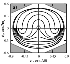
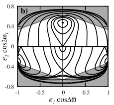
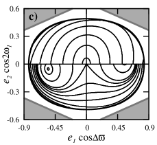
Figure 4: Levels of the secular Hamiltonian in the quadrupole approximation (top panels), and in the octupole approximation (bottom panels). These plots are obtained for $\alpha=0.333$, $\mu=0.5$ and ${\mathcal{\cal A}}=0.1$ (the left-hand panels), and ${\mathcal{\cal A}}=0.25$ (the right hand panels). Compare with the semi-analytic model in Fig. 3. The shaded areas mark parameters for which the expansion of ${\cal H}_{\mbox{\scriptsize sec}}$ in terms of $\alpha$ would diverge.

3.2 Lyapunov stability and critical inclinations

The stability of equilibria may be investigated with the help of Lyapunov theorem (see, e.g., Markeev, 1978; Khalil, 2001). If the Hamiltonian is positive (negative) definite function in a neighborhood of an equilibrium ${\bf x}_{0}$, then the equilibrium is Lyapunov stable. At a stable equilibrium, the parameters of the averaged system are constant, hence the orbital elements do not change in the secular-time scale, and the orbital con figuration evolves in the short-time scale only. In the 3-D secular problem, that is equivalent to conditions for local extrema of ${\cal H}_{\mbox{\scriptsize sec}}$ in the phase space. We recall that such extrema must appear as elliptic points in 2-D plots of the $\cal S$-plane. We should also remember that these quasi-elliptic points may be in fact related to saddles in two remaining and “hidden” dimensions of the phase space. To determine, whether the secular Hamiltonian is sign definite function of the phase variables in the neighborhood of a critical point, we compute its Hessian, ${\mathbb{H}}_{2}=\partial^{2}\,{\cal H}_{\mbox{\scriptsize sec}}/\partial\,{\bf x}^{2}$ at the equilibrium, and then we determine whether it is sign-definite matrix.

As an illustration, we show two plots of the sub-determinants of Hessian ${\mathbb{H}}_{2}$ in Fig. 5 which are computed at the origin as functions of the mutual inclination of circular orbits, $i_{0}$. The top-panel is for $\alpha=0.333$, $\mu=2$ and the bottom panel is for $\alpha=0.667$, $\mu=2$. For some particular values of $i_{0}$, which are related to the given value of ${\mathcal{\cal A}}$, the sub-determinants may vanish and then we cannot determine sign-definiteness of the Hessian. For instance, if $\alpha=0.333$ then it takes place for $i_{0}$ close to $\sim 45^{\circ}$, $70^{\circ}$, $130^{\circ}$, and $155^{\circ}$, respectively.

In fact, these values of $i_{0}$ are related to bifurcational inclinations of the “trivial” equilibrium at the origin (Krasinsky, 1972, 1974) and changes of its stability and global topology of ${\cal H}_{\mbox{\scriptsize sec}}$. The later work gives explicitly their values in terms of parameter $\beta\equiv L_{1}/L_{2}\sim\mu\sqrt{\alpha}$ which were calculated for the second order secular Hamiltonian (the quadrupole term). For a reference, the vertical lines in Fig. 5 mark the bifurcations derived with the quasi-analytic theory (thin lines), and with the quadrupole Hamiltonian (thick, dashed lines). Bifurcational values of $i_{0}$ are labeled with $I^{+,-}_{1,2,3,4}$. Following terminology of Krasinsky (1974), the “+” sign means that the bifurcation of the origin leads to nontrivial solution of the positive type, the “–” sign means nontrivial solution of the negative type. The positive type solutions are characterized by $\omega_{1,2}=0,\pi$, hence bifurcations take place in the ${\cal P}_{C}$-plane; the negative type equilibria ($\omega_{1,2}=\pm\pi/2$) appear after bifurcations in the ${\cal P}_{S}$-plane. An inspection of Fig. 5 reveals, that the bifurcational inclinations may be very different in both theories, and it may be particularly well seen for $\alpha=0.667$ (bottom panel of Fig. 5). In the later case, the bifurcational values of inclination are clearly splitted, and the bifurcations takes place for different ${\mathcal{\cal A}}$ (or $J_{1}\equiv C$). Note that they only depend on $\beta$ in the quadrupole theory, and on $\mu$ and $\alpha$ separately in the full model. Actually, angles $I_{1}^{+}=I_{1}^{-}$ and $I_{2}^{-}=I_{2}^{+}$ are degenerated in the quadrupole theory (note that the octupole theory breaks the symmetry). All that means that the topology of the phase space must be different in the two secular theories.

When the Hamiltonian evaluated at a critical point is not a sign definite function then the analysis of stability become much more difficult than in the case of an extremum. In general, only the linear stability of the equilibrium can be determined relatively easy. We accomplish that by solving the eigenproblem of matrix ${\mathbb{A}}$ of the linearized equations of motion. The variational equations in terms of new canonical variables ${\bf y}$, where ${\bf x}={\bf x}_{0}+{\bf y}$:

$${\frac{\mbox{d}{\bf y}}{\mbox{d}t}}={\mathbb{A}}\,{\bf y},\quad{\mathbb{A}}={\mathbb{I}}\,{\mathbb{H}}_{2}({\bf x}_{0}),$$

and ${\mathbb{I}}$ is the symplectic unit. In general, for a conservative Hamiltonian system, ${\mathbb{A}}$ has complex eigenvalues

$$\lambda_{i}=\pm\rho_{i}\pm\mbox{i}\sigma_{i},\quad\rho_{i},\sigma_{i}\in{\mathbb{R}},\quad\rho_{i}\geq 0,\quad\sigma_{i}\geq 0,\quad i=1,2.$$

We can find them easily as the roots of symmetric characteristic polynomial $p(\lambda)=\det({\mathbb{A}}-\lambda{\mathbb{E}})=0$, where ${\mathbb{E}}$ is the unit matrix. It is well known that the necessary and sufficient condition for the linear stability is fulfilled if $\lambda_{i}=\pm\mbox{i}\sigma_{i}$ are purely imaginary and matrix ${\mathbb{A}}$ is diagonalizable ($\sigma_{i}$ are the characteristic frequencies).

In the case of two-degree of freedom conservative Hamiltonian systems, we can apply the theorem of Arnold–Moser (e.g., Meyer & Schmidt, 1986) to conclude that equilibria which are linearly stable are generically Lyapunov stable. However, there is no such implication if the characteristic frequencies are involved in resonances up to the 4-th order, i.e., when $p\sigma_{1}+q\sigma_{2}=0$ for $0<|p|+|q|\leq 4$, with $p,q\in\mathbb{Z}$, or when coefficients of the Birkhoff’s normal form of the Hamiltonian expanded near the equilibrium fulfill a particular condition involving $\sigma_{i}$ [see (Meyer & Schmidt, 1986) or (Markeev, 1978) for details]. In resonant cases, we should examine each particular normal form of the polynomial expansion of the Hamiltonian with respect to variations ${\bf y}$. This can be done with the help of constructive theorems by Markeev and Sokolskii [see, e.g., Markeev (1978); Sokolskii (1975) or Goździewski (2003b) for an example application of these theorems, and references therein]. Moreover, because high-order expansions are required, such an extensive study is hardly possible because we must average out ${\cal H}_{\mbox{\scriptsize sec}}$ and calculate its derivatives numerically. A precise enough determination of the second order derivatives becomes very difficult. Hence, we are forced to limit the stability analysis to the linear, non-resonant case. Nevertheless, recalling the implications of the Arnold-Moser theorem, a study of the linear stability provides valuable information on the generic Lyapunov stability.

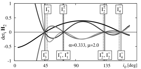
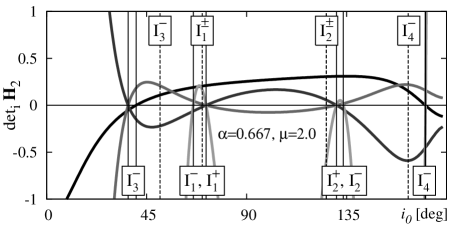
Figure 5: The sub-determinants of the Hessian of the secular Hamiltonian, $\det_{1}{\mathbb{H}}_{2}$, $\det_{2}{\mathbb{H}}_{2}$, $\det_{3}{\mathbb{H}}_{2}$ and $\det_{4}{\mathbb{H}}_{2}$ evaluated at the origin of the $\cal S$-plane. The sub-determinants are plotted with gradually shaded curves as functions of ${\mathcal{\cal A}}$ or $i_{0}$, starting with the black curve for $\det_{1}{\mathbb{H}}_{2}$, and lightest gray curve for $\det_{4}{\mathbb{H}}_{2}$. The sub-determinants are expressed in relative units. The vertical lines mark the bifurcational mutual inclinations of orbits at the origin ($i_{0}$) that correspond to $\det_{i}{\mathbb{H}}_{2}=0$ for one (or more) $i=1,2,3,4$. These inclinations are labeled with $I^{+,-}_{1,2,3,4}$. Thin, dashed, vertical lines labeled at the top are for the quadrupole order theory, and the thin solid lines labeled at the bottom are for the semi-analytic theory. See the text for more details.

3.3 A general view of the $\cal S$-plane

While in Sect. 4 we describe the results regarding new families of stationary solutions found in this paper in some systematic way, here we refer to generic properties of the $\cal S$-plane identified through many numerical experiments. Fixing ${\mathcal{\cal A}}$, we can obtain typical views of the $\cal S$-plane which are shown in three panels of Fig. 3. The left panel of Fig. 3 illustrates configurations recently investigated in Michtchenko et al. (2006) and Libert & Henrard (2007b). We can see a maximum of ${\cal H}_{\mbox{\scriptsize sec}}$ at quadrant IV ($\omega_{1}=\pi/2$, $\omega_{2}=\pi/2$) of the $\cal S$-plane. It corresponds to equilibrium marked with IVa and known as the Lidov-Kozai resonance, with the analogy to the restricted problem (Lidov, 1961; Kozai, 1962). In the vicinity of equilibrium IVa of the non-restricted problem, angles $\omega_{1}$ and $\omega_{2}$ librate around $\pi/2$. Simultaneously, these librations of $\omega_{1,2}$ are related to large-amplitude, anti-phase variations of the eccentricity of the inner orbit and of the mutual inclination. This mechanism may lead to strong instability. We observed it already in the case of hierarchical two-planet configurations (Goździewski & Konacki, 2004).

Due to discontinuity of the ${\cal P}_{M}$-plane at the $x$-axis, it is difficult to follow the evolution of geometric structure of the L-K resonance. Instead, the ${\cal P}_{S}$ and ${\cal P}_{C}$ representative planes are more convenient for that purpose, particularly near the origin. A sequence of plots shown in Fig. 6, reproduces the analytical results of Libert & Henrard (2007b) which were obtained for $\alpha=0.1$ and $\mu=0.25$. For ${\mathcal{\cal A}}=0.01$ (the left-hand panel of Fig. 6), the origin is stable, permitting mutual inclination of circular orbits $i_{0}\sim 30^{\circ}$. With increasing ${\mathcal{\cal A}}=0.03$, the inclination grows, and for $i_{0}\sim 43^{\circ}$, the stable stationary point become unstable and bifurcates. Three new solutions appear: one is unstable and two are stable. This phenomenon may be called the L-K bifurcation. At the bifurcation point, some sub-determinants of ${\mathbb{H}}_{2}$ are equal to zero and the stability cannot be determined (see Fig. 5 and the previous Section for details). With further increase of ${\mathcal{\cal A}}$, the L-K resonance centers move toward large values of $e_{1}$ (see the third panel in Fig. 6 plotted for ${\mathcal{\cal A}}=0.06$) and approach $e_{1}\sim 1$ for ${\mathcal{\cal A}}=0.08$ (see the last, fourth panel in Fig. 6). While we refer to the analytic work of (Libert & Henrard, 2007b), these authors did not follow the L-K equilibrium for this value of ${\mathcal{\cal A}}$. The semi-analytical algorithm makes it possible to continue the family of L-K solutions up to such a value, for which we observe new bifurcations of the equilibria. From each bifurcation of stable L-K equilibrium emerge three new solutions: one linearly stable (a saddle point in the $\cal S$-plane) and two elliptic points. One of them is Lyapunov stable, the other one is unstable. The elliptic points approach $e_{1}\sim 1$ and moderate $e_{2}$. The solution at the origin bifurcates the second time but it remains unstable (note that it appears as an elliptic point in the $\cal S$-plane) and two unstable equilibria (saddles of ${\cal H}_{\mbox{\scriptsize sec}}$) located at $(e_{1}\sim 0,e_{2}>0)$ also appear.

In the second plot of the $\cal S$-plane (see the middle panel of Fig. 3), we consider a configuration with $\alpha=0.333$, $\mu=0.5$ for ${\mathcal{\cal A}}=0.25$. We can recognize the L-K resonance after a bifurcation: the bottom-left quadrant of the $\cal S$-plane reveals a local extremum labeled with IVa and a saddle point IVb-. In remaining three quadrants, we can find also other new equilibria labeled with IIa, IIb, IIIa, IIIb, respectively. Curiously, the maximum marked with IIa lies beyond the geometrical crossing line of orbits defined implicitly through $a_{1}(1\pm e_{1})=a_{2}(1-e_{2})$. Finally, in the right-hand panel of Fig. 3, we draw the ${\cal P}_{M}$-plane for large ${\mathcal{\cal A}}=0.85$ which lead to a discontinuity of the energy plane in the regime of large $e_{2}$. In this case, the inclination reaches very large values.

These examples indicate that the 3-D problem is much more complex and rich in dynamical phenomena than the co-planar problem of two planets. We recall that in this case (Michtchenko & Malhotra, 2004), the phase space of the secular system is spanned by librations of $\Delta\varpi$ around $0$ (mode I), librations of $\Delta\varpi$ around $\pi$ (mode II), and circulations of $\Delta\varpi$. There is also possible the so called non-linear secular resonance (the true secular resonance) which is present in the regime of moderate and large eccentricities.

Generally, the equilibria are not isolated in the parameter space of ($\mu,\alpha)$ and the $\mathrm{AMD}$ integral. Yet, as the example of the L-K resonance demonstrates, the stationary solution may evolve in the parameter space, they can bifurcate, and may change their stability. Hence they form families of solutions and their behavior depends on a complex way on problem parameters. To investigate these families, we require a continuation method for determining bifurcations of the equilibria and their stability.

       

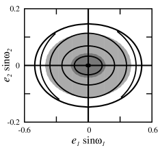
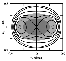
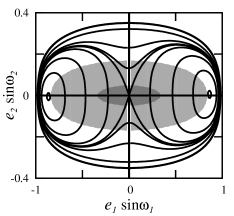
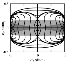
Figure 6: Levels of the secular energy (${\cal H}_{\mbox{\scriptsize sec}}$) at the ${\cal P}_{S}$-plane defined through $(e_{1}\sin{\omega_{1}},~{}e_{2}\sin{\omega_{2}})$ with $\omega_{1},\omega_{2}=\pm\pi/2$, for $\alpha=0.1$, $\mu=0.25$ and ${\mathcal{\cal A}}$ are (from the left-hand panel to right-hand panel): $0.01,0.03,0.06,0.08$, respectively. Shaded areas indicate ranges of the mutual inclination: $(0^{\circ},20^{\circ},30^{\circ})$ for the left-hand panel, $(0^{\circ},50^{\circ},60^{\circ})$ and $(0^{\circ},70^{\circ},80^{\circ})$ for the inner panels, respectively, and $(0^{\circ},95^{\circ},105^{\circ})$ for the right-hand panel.

4 Parametric survey of equilibria

To resolve the families of equilibria, we apply a simple continuation method with respect to ${\mathcal{\cal A}}$ as the primary parameter. For fixed parameters $\alpha$ and $\mu$, ${\mathcal{\cal A}}\in[0,1]$. We increase this quantity by small steps, and we compute the secular energy map in the $\cal S$-plane. An inspection of the characteristic plane makes it possible to detect the origin and development of basic dynamical structures. In particular, we can determine critical values of ${\mathcal{\cal A}}$ for which new equilibria (represented by elliptic or saddle points in the $\cal S$-plane) appear (see, e.g., Fig. 6). Having an overall view of the $\cal S$-plane, we may follow a given solution along some path in the parameters space with the help of a minimization algorithm (see below).

Here, we show two example sets of the $\cal S$-plane derived for two pairs of $(\alpha,\mu)$. Figures 7–9 are for $(\alpha,\mu)\equiv(0.333,0.5)$, while figures 10–11 are for $(\alpha,\mu)\equiv(0.2,2)$. We start to look more closely at the first set of the energy diagrams. Figure 7 comprises of a number of panels derived for varied values of ${\mathcal{\cal A}}$. Each value of ${\mathcal{\cal A}}$ is related to the mutual inclination at the origin, $i_{0}$. Shaded ares in these plots mark ranges of the mutual inclination permitted by the given and fixed ${\mathcal{\cal A}}$. Lighter shadings encode smaller mutual inclinations. Thin black curves encompass the region of permitted motion according with ${{\cal I}_{\mbox{\scriptsize mut}}}=0,\pi$. We show the $\cal S$-plane defined as ${\cal P}_{M}$ (see Fig. 7) as well as the ${\cal P}_{S}$-plane (Fig. 8) and ${\cal P}_{C}$-plane (Fig. 9). We can see very clearly that the ${\cal P}_{S,C}$-planes provide a continuous representation of energy levels.

A sequence of energy diagrams shown in Figs. 7–9 helps us to understand the development of a few families of equilibria found in this work. We start with ${\mathcal{\cal A}}=0.03$ (the top left-hand panel). In this case, the origin is the global extremum (the maximum) of the secular energy. This corresponds to the well known classic zero-eccentricity equilibria investigated in detail in (Krasinsky, 1972, 1974; Libert & Henrard, 2007b). When ${\mathcal{\cal A}}=0.1$ (the next panel in the top row), we see a saddle at the origin and a maximum in quadrant IV of ${\cal P}_{M}$-plane, which can be better seen in the ${\cal P}_{S}$-plane. The extremum can be identified with the Lidov-Kozai resonance. Clearly, in that case, the neighboring trajectories characterized by librations of angle $\omega_{1}$ around $\pi/2$. We can also notice a non-classic feature, regarding the non-restricted model of the L-K resonance: close to the quasi-elliptic point, also angle $\Delta\varpi$ may librate around $\pi$ (it means that $\omega_{2}$ librates around $\pi/2$). This effect is possible for compact systems.

When ${\mathcal{\cal A}}=0.18$ (the next panel in the top row of Figs. 7–9), new structures appear: a saddle at the origin of the ${\cal P}_{C}$-plane (see appropriate panel in Fig. 9) with two elliptic points close to the $e_{1}=0$ axis, as well as an elliptic point above the collision line (marked with thin lines). The change of topology of ${\cal H}_{\mbox{\scriptsize sec}}$ is also visible in the respective panels of the ${\cal P}_{S}$-plane. As we already noticed, it is related to the second bifurcation of the origin. Simultaneously, the center of the L-K resonance moves toward large $e_{1}$. When the ${\mathcal{\cal A}}=0.25$ (the top right-hand panel of Fig. 8) we observe a further development of the structure around the origin and a bifurcation of the extremum identified with the L-K resonance onto a saddle point and two new elliptic points appearing in the regime of large $e_{1}$. These structures are particularly well seen in ${\cal P}_{S,C}$-planes, respectively, as illustrated in Fig. 8 and Fig. 9.

A similar analysis might be carried out for the second set of parameters $(\mu,\alpha)$. We do not present it in detail, however an inspection of the energy diagrams shown in Fig. 10, and Fig. 11 reveals that the sequence of plots ends in a different dynamical situation: even for large ${\mathcal{\cal A}}$, the region of permitted motion remains closed. Obviously, the evolution of equilibria appearing for the second pair of parameters ($\alpha,\mu$) is different from the first case.

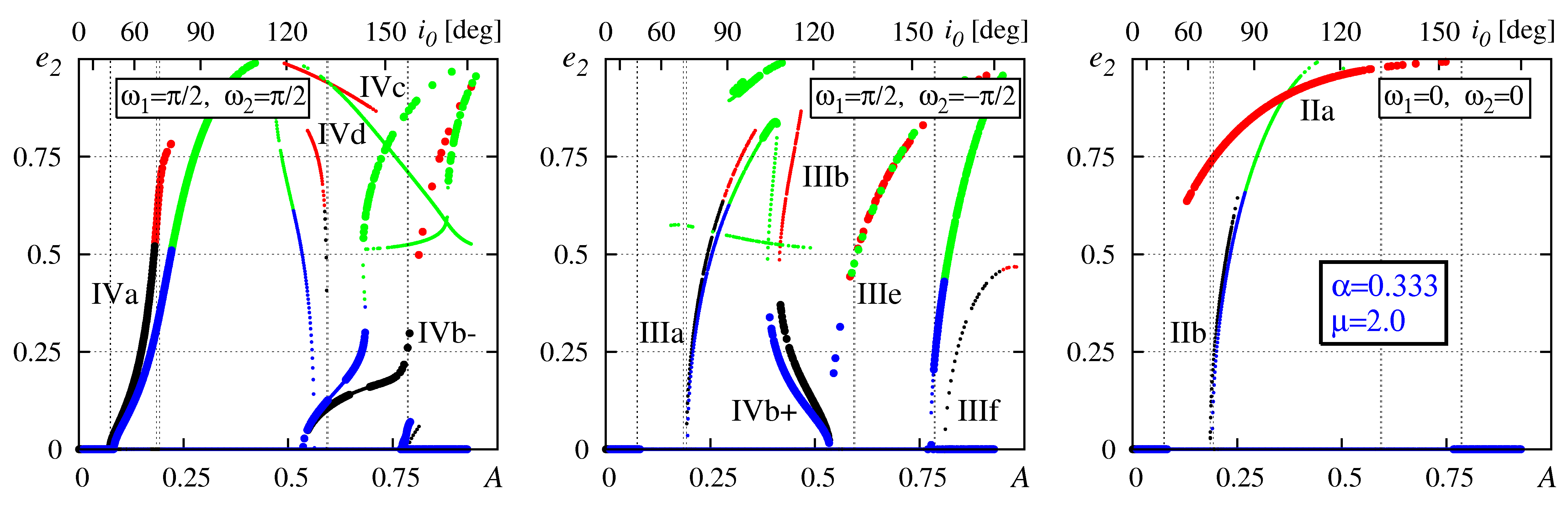
Figure 12: A comparison of families of stationary solutions found with the octupole expansion of the secular Hamiltonian (green and blue filled circles) and with the help of quasi-analytic method (black and red filled circles). Parameters are for $\alpha=0.333$ and $\mu=2$. Large filled circles are for stable solutions, and smaller circles are for unstable equilibria. The red and green filled circles are for equilibria beyond the formal convergence limit of ${\cal H}_{\mbox{\scriptsize sec}}$ expanded in $\alpha$.

Finally, we consider one more experiment devoted to a comparison of the results derived with the help of the octupole theory and the quasi-analytic averaging algorithm. Figure 12 illustrates a few families of equilibria derived for $\alpha=0.333$ and $\mu=2$. Black and red filled circles are for the semi-analytic theory, blue and green filled circles are for the octupole Hamiltonian approximation. The red and green points indicate equilibria found beyond the formal limit of convergence of the expansion of ${\cal H}_{\mbox{\scriptsize sec}}$ in $\alpha$. We may notice significant differences between some branches of equilibria already in the regime of moderate $e_{2}$. There are also solutions permitted by the octuple theory, represented by green horizontal branches, which are absent in the quasi-analytic model. This test confirms that the study of equilibria in compact systems benefit from the application of the semi-analytic (basically exact) averaging.

Hence, we should follow a more systematic procedure. Once we identify a solution of a given family for fixed pair of ($\alpha,\mu$), we may continue that family by searching for the zeros of the right hand sides of the equations of motion, Eqs. 15. This task may be accomplished by minimization of the norm of the partial derivatives of the secular Hamiltonian. To speed up the minimization, we apply the fast Levenberg-Marquardt algorithm (Press et al., 1992). Simultaneously, we examine the stability of solutions which are found after the L-M algorithm converged. Perhaps a more elaborate algorithm of the continuation of the equilibria might be applied, nevertheless, even with such a simple approach, we are able to identify a few families of solutions that are, to the best of our knowledge, unknown in the literature. Finally, Figs. 13–15 illustrate the results of the continuation globally. Each set of panels is derived for fixed $(\mu,\alpha)$ chosen as combinations of parameters $\alpha=0.2$, $0.333$, $0.667$ and $\mu=0.25$, $0.5$, $1$, $2$, respectively. The continuation of the families of equilibria is done in the whole possible range of ${\mathcal{\cal A}}$. We plot ${{\cal I}_{\mbox{\scriptsize mut}}}$, $e_{1}$ and $e_{2}$ of the found stationary solutions, as functions of ${\mathcal{\cal A}}$ (and, if the value of ${\mathcal{\cal A}}$ permit circular orbits, as a function of $i_{0}$). Columns in each group of diagrams are for particular quadrants of the $\cal S$-plane. Note, that we skipped panels for quadrant I because in that quadrant we found only one family Ia of unstable solutions for a limited range of $\mu\geq 1$ (see Sect. 4.2 for details). Simultaneously, Lyapunov stable (or linearly stable) equilibria are marked with large filled circles, and unstable solutions are marked with small filled circles. Families of equilibria are classified accordingly with the quadrant of $\cal S$-plane in which they appear, and they are labeled with corresponding Roman numbers. Let us note that the red filled circles indicate equilibria found beyond the formal limit of convergence of the expansion of ${\cal H}_{\mbox{\scriptsize sec}}$ in $\alpha$.

In this way, we can obtain quite a deep insight into the secular equilibria and their stability in wide ranges of the primary parameters. Below, we describe the identified families of stationary solutions in more detail, and we try to characterize the associated dynamical behaviors of the secular system. A likely position of the HD 12661 system in the diagrams Figs. 13–15 may be deduced from its currently known orbital elements, $\alpha\sim 0.3$ and $\mu\sim 1$. For relatively small ${\mathcal{\cal A}}\sim 0.1$, the system might be found in the top, right-hand panels of Fig. 14, in the regime of the L-K bifurcation, still with moderate $e_{1}\sim 0.3$ and $e_{2}\sim 0.1$.

               

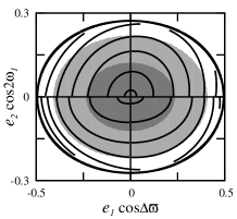
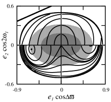
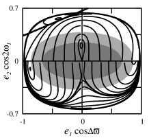
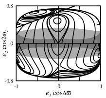
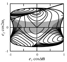
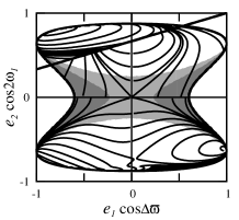
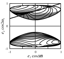
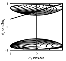
Figure 7: Levels of the secular energy (${\cal H}_{\mbox{\scriptsize sec}}$) at the ${\cal P}_{M}$-plane defined through $(e_{1}\cos{\Delta\varpi},~{}e_{2}\cos{2\omega_{1}})$ with $\Delta\varpi=0,\pi$, $2\omega_{1}=0,\pi$, for $\alpha=0.333$, $\mu=0.5$ and varied ${\mathcal{\cal A}}$ (or the mutual inclination of circular orbits, $i_{0}$). Values of ${\mathcal{\cal A}}$ are (counting plots from the left to the right and from the top to the bottom): $0.03,0.1,0.18,0.25,0.33,0.4,0.46,0.50$, respectively. Each panel has two shaded regions indicating ranges of the mutual inclinations (corresponding to the fixed above of ${\mathcal{\cal A}}$): $(20^{\circ},30^{\circ})$, $(50^{\circ},60^{\circ})$, $(70^{\circ},80^{\circ})$, $(95^{\circ},105^{\circ})$, $(120^{\circ},130^{\circ})$, $(140^{\circ},150^{\circ})$, and $(130^{\circ},140^{\circ})$, $(120^{\circ},130^{\circ})$, respectively.

               

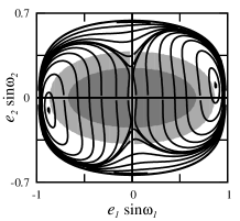
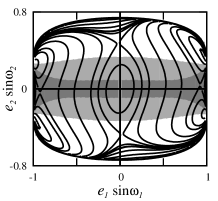
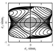
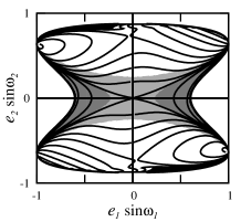
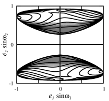
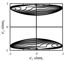
Figure 8: The energy levels plotted in the ${\cal P}_{S}$ representative plane of $(e_{1}\sin{\omega_{1}},~{}e_{2}\sin{\omega_{2}})$ with $\omega_{1},\omega_{2}=\pm\pi/2$. Parameters are $\alpha=0.333$, $\mu=0.5$, the values of ${\mathcal{\cal A}}$ and inclination ranges are the same as in Fig. 7.

               

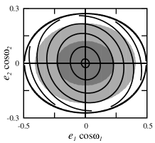
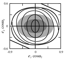
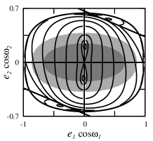
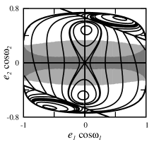
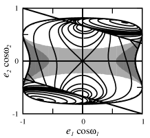
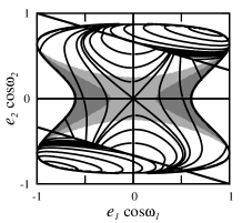
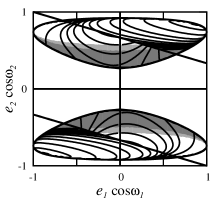
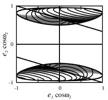
Figure 9: The energy levels plotted in the ${\cal P}_{C}$ representative plane of $(e_{1}\cos{\omega_{1}},~{}e_{2}\cos{\omega_{2}})$ with $\omega_{1},\omega_{2}=0,\pi$. Parameters are $\alpha=0.333$, $\mu=0.5$, the values of ${\mathcal{\cal A}}$ and inclination ranges are the same as in Fig. 7.

                       

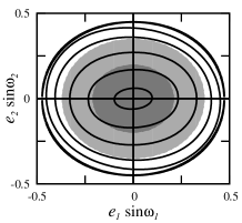
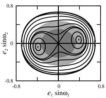
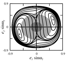
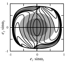
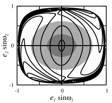
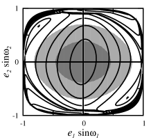
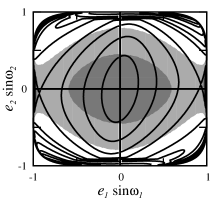
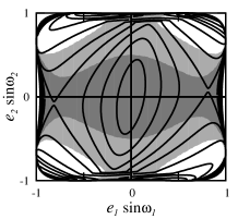
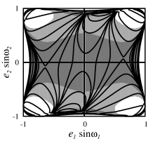
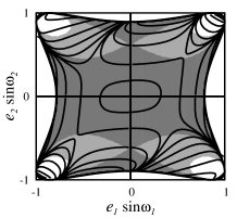
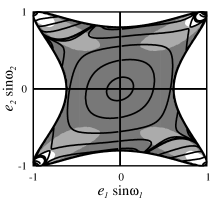
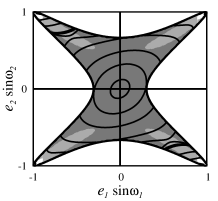
Figure 10: Levels of the secular energy (${\cal H}_{\mbox{\scriptsize sec}}$) at the ${\cal P}_{S}$-plane defined through $(e_{1}\sin{\omega_{1}},~{}e_{2}\sin{\omega_{2}})$ with $\omega_{1},\omega_{2}=\pm\pi/2$, for $\alpha=0.2$ and $\mu=2.0$ and for varied ${\mathcal{\cal A}}$ values. From the left to the right and from the top to the bottom: $0.06,0.13,0.21,0.29$ (the top row), $0.37,0.45,0.53,0.61$ (the middle row), and $0.69,0.76,0.84,0.92$ (the bottom row), respectively. Shaded regions illustrate mutual inclinations in prescribed ranges (lower inclination — lighter shade, larger inclination — darker shade). For each fixed value of ${\mathcal{\cal A}}$, there are two levels of $I_{mut}$ which are marked in subsequent panels: $(25^{\circ},35^{\circ})$, $(45^{\circ},55^{\circ})$ $(65^{\circ},75^{\circ})$, $(75^{\circ},85^{\circ})$ for the upper row; $(90^{\circ},100^{\circ})$, $(100^{\circ},110^{\circ})$, $(110^{\circ},120^{\circ})$, $(120^{\circ},130^{\circ})$ for the middle row; $(130^{\circ},140^{\circ})$, $(140^{\circ},150^{\circ})$, $(150^{\circ},160^{\circ})$, $(160^{\circ},170^{\circ})$ for the bottom row, respectively.

                       

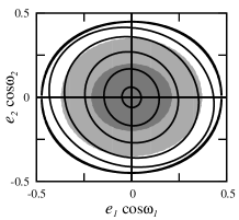
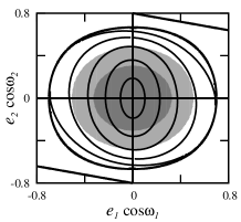
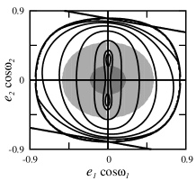
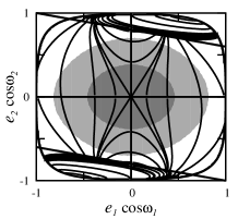
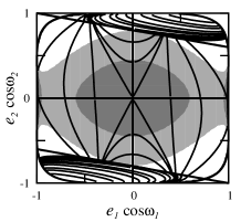
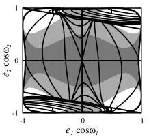
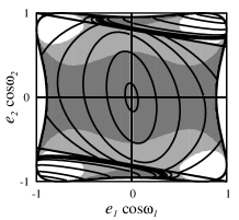
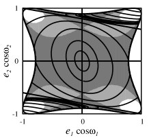
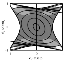
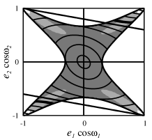
Figure 11: Levels of ${\cal H}_{\mbox{\scriptsize sec}}$ for orbital parameters specified in caption to Fig. 10 and plotted in the ${\cal P}_{C}$-plane of $(e_{1}\cos{\omega_{1}},~{}e_{2}\cos{\omega_{2}})$, where $\omega_{1},\omega_{2}=0,\pi$. Values of ${\mathcal{\cal A}}$ and ranges of mutual inclinations are the same as in that figure.

4.1 Family 0 at ${\mathbf{(e_{1},e_{2})=(0,0)}}$

The stationary solution at the origin $(e_{1}=0,e_{2}=0)$ (see an example in Fig. 6) was investigated in detail by Libert & Henrard (2007b) for $\alpha=0.1$, $\mu=0.25$, i.e., for relatively distant orbits (or typically hierarchical configuration). In our classification, this family is marked with ”0” in all stability diagrams of Figs. 13–15. Solutions of this family are also studied in detail by Krasinsky (1972, 1974) in terms of the quadrupole approximation of ${\cal H}_{\mbox{\scriptsize sec}}$, and we already did many references to these works and its results. Here, we start to follow more closely the evolution of family ”0” for $(\alpha,\mu)\equiv(0.333,0.5)$ with respect to ${\mathcal{\cal A}}$. Similarly, Fig. 10 and Fig. 11 reveal topology of the $\cal S$-plane and the evolution of zero-eccentricity equilibria for a different pair of parameters, $(\alpha,\mu)\equiv(0.2,2)$.

When the mutual inclination remains relatively small (see Figs. 7–9), the zero-eccentricity equilibrium is Lyapunov stable because it corresponds to the maximum of ${\cal H}_{\mbox{\scriptsize sec}}$. When ${\mathcal{\cal A}}$ increases, a bifurcation of this solution appears for $i_{0}\sim 43^{\circ}$ (as mentioned already, the L-K bifurcation). Inspecting the ${\cal P}_{S}$-plane (Fig. 8), we may notice that at the bifurcation point a new family IVa appears, and it remains Lyapunov stable up to extremely large $e_{1}$. After $e_{1}$ reaches the limit of 1 (simultaneously, the mutual inclination is close to $\pi/2$), the family bifurcates again: the family IVa remains on a branch with large $e_{1}$ while a new branch of solutions (family IVb-) can be continued to large mutual inclinations with simultaneous decrease of $e_{1}$. Family IVb- can be regarded as the retrograde case of the L-K resonance with ${{\cal I}_{\mbox{\scriptsize mut}}}>\pi/2$. Note that families IVa and IVb- are quasi-symmetric with respect to ${{\cal I}_{\mbox{\scriptsize mut}}}\sim\pi/2$, regarding the eccentricity and inclination of the inner orbit. This symmetry is more ”exact” for smaller $\alpha$ (hierarchical configurations). We notice, that the quadrupole term approximation leads to exact symmetry of the equilibria (see Fig. 4 and the relevant comments in Sect. 4.3).

We may also discover unstable family IIIb, which has the elliptic point located in quadrant III as well as a saddle of family IVb+ corresponding to linearly stable solution. In the later case, the neighboring trajectories are characterized by librations of $\omega_{1}$ around $\pi/2$ and also (within a limited vicinity of the libration center), by librations of $\omega_{2}$ around $-\pi/2$. A further increase of ${\mathcal{\cal A}}$ leads to a shift of solutions IVa, IVb-, and IIIb towards the border of permitted motions. Finally, for ${\mathcal{\cal A}}>0.4$, the zero-eccentricity equilibria vanish at all, and the energy plane is divided onto two distinct islands. By inspecting the ${\cal P}_{C}$-plane (see the third panel in top row in Figs. 7,9 and 11) we can also detect the second bifurcation of the zero-eccentricity equilibria which is associated with the apparence of a saddle at the origin accompanied by two unstable elliptic points close to $e_{1}\sim 0$. These solutions can be classified as members of family IIb because they emerge in quadrant II of the $\cal S$-plane. The saddles visible in ${\cal P}_{S}$ (Fig. 8) represent members of family IIIa [see also Fig. 10 for the second pair of $(\alpha,\mu)$].

Thanks to the semi-numerical algorithm, we can follow the zero-eccentricity family not only for larger $\alpha$, up to 0.667, but also in wide ranges of the mass ratios, between $0.25$ and $2$. Stability diagrams in Figs. 13–15 illustrate bifurcations of equilibria for different parameter pairs. Obviously, the zero-eccentricity solutions appear for all combinations of the primary parameters, moreover, the evolution of this family is very complex. Bifurcations of family “0” lead to new classes of equilibria and qualitative changes of the ${\cal H}_{\mbox{\scriptsize sec}}$ topology as seen at the $\cal S$-plane.

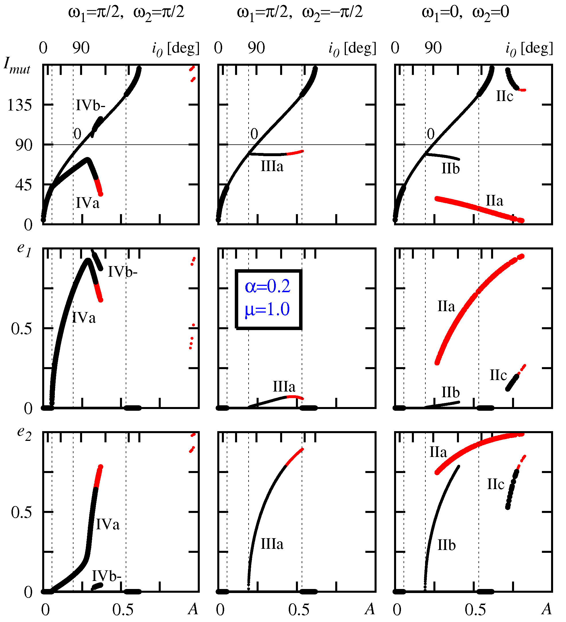
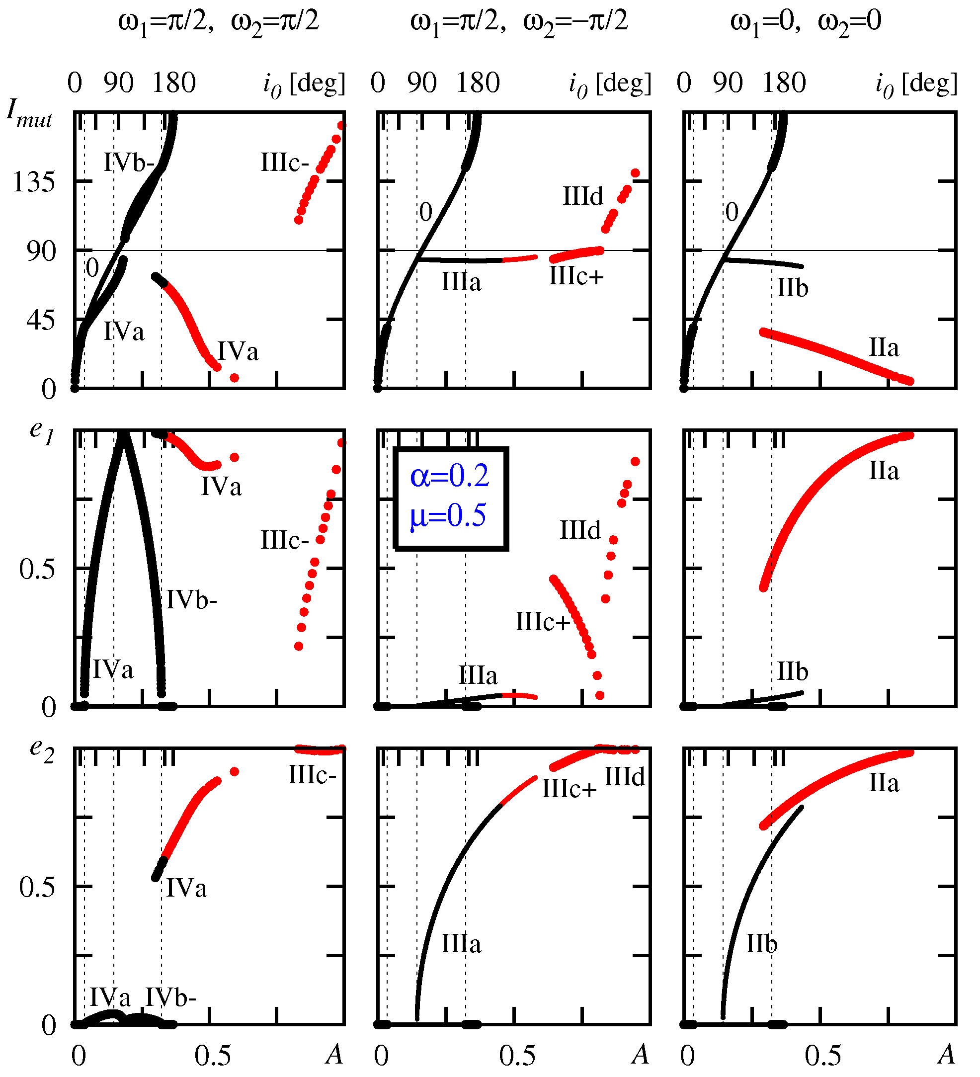
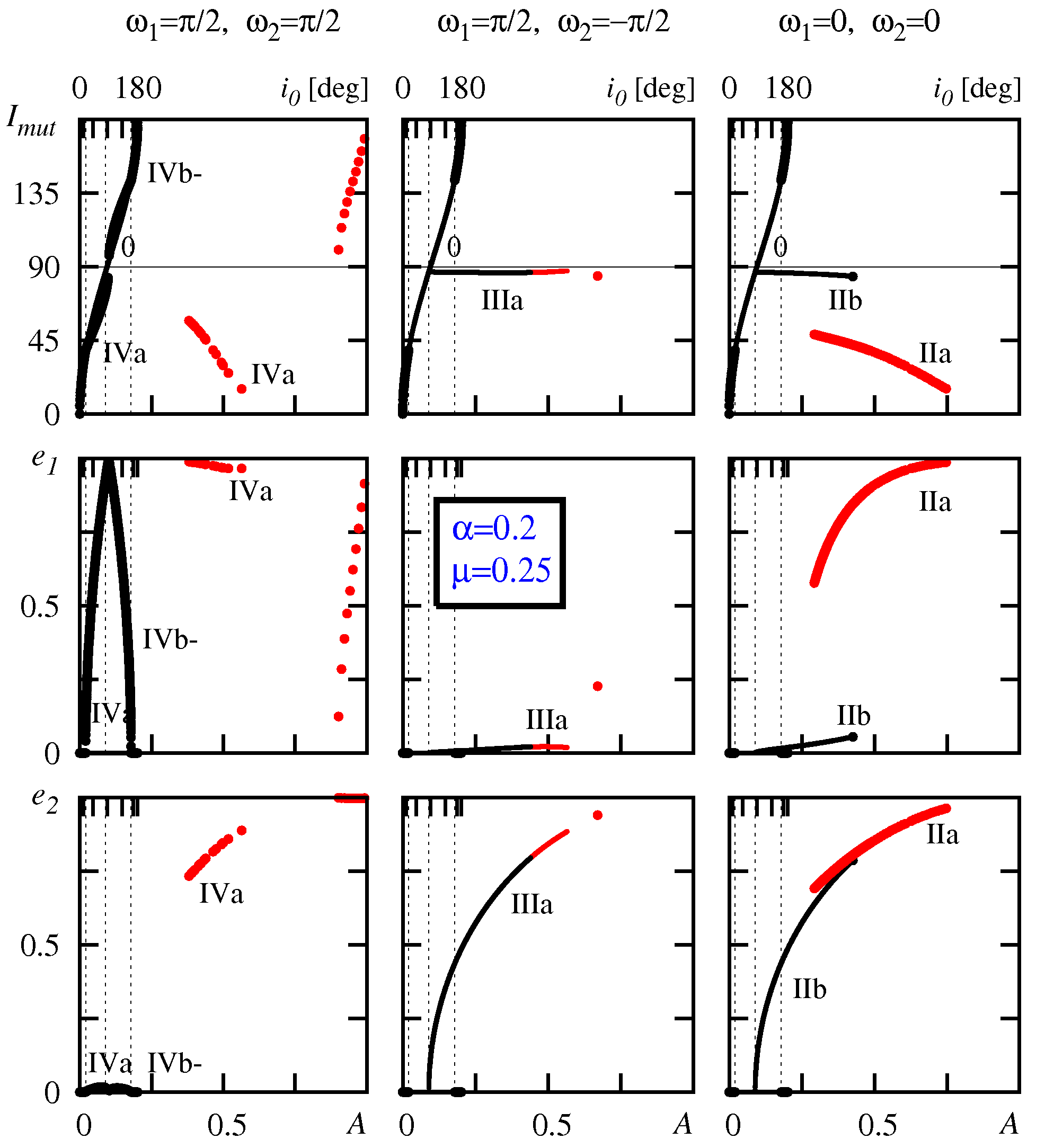
Figure 13: Families of stationary solutions obtained for $\alpha=0.2$ and the following mass ratios: $\mu=2.0$ – the top left-hand plots, $\mu=1.0$ – the top right-hand plot, $\mu=0.5$ – the bottom left-hand, and $\mu=0.25$ – the bottom right-hand plots. Large filled circle are for Lyapunov stable (or linearly stable) equilibria, smaller filled circles are for unstable equilibria, red filled circles are for solutions found in regions, where the power series of ${\cal H}_{\mbox{\scriptsize sec}}$ in $\alpha$ would diverge. The stationary solutions are classified according with the quadrant of the $\cal S$-plane, in which they appear, hence the columns in each sub-group of diagrams [for fixed $(\alpha,\mu$) written in the legend] are for the following $(\omega_{1},\omega_{2})$-pairs: $(\pi/2,\pi/2)$ – the left column, $(\pi/2,-\pi/2)$ – the middle column, and $(0,0)$ – the right column. Each sub-group of stability diagrams has panels for the mutual inclination (the top row), and for the eccentricities (the middle and the bottom rows, respectively). The $x$-axis of each diagram is labeled by ${\mathcal{\cal A}}$ and $i_{0}$. Particular families of solutions which are identified in this work are labeled with Roman numbers and appropriate Latin letters. See the text for more details.

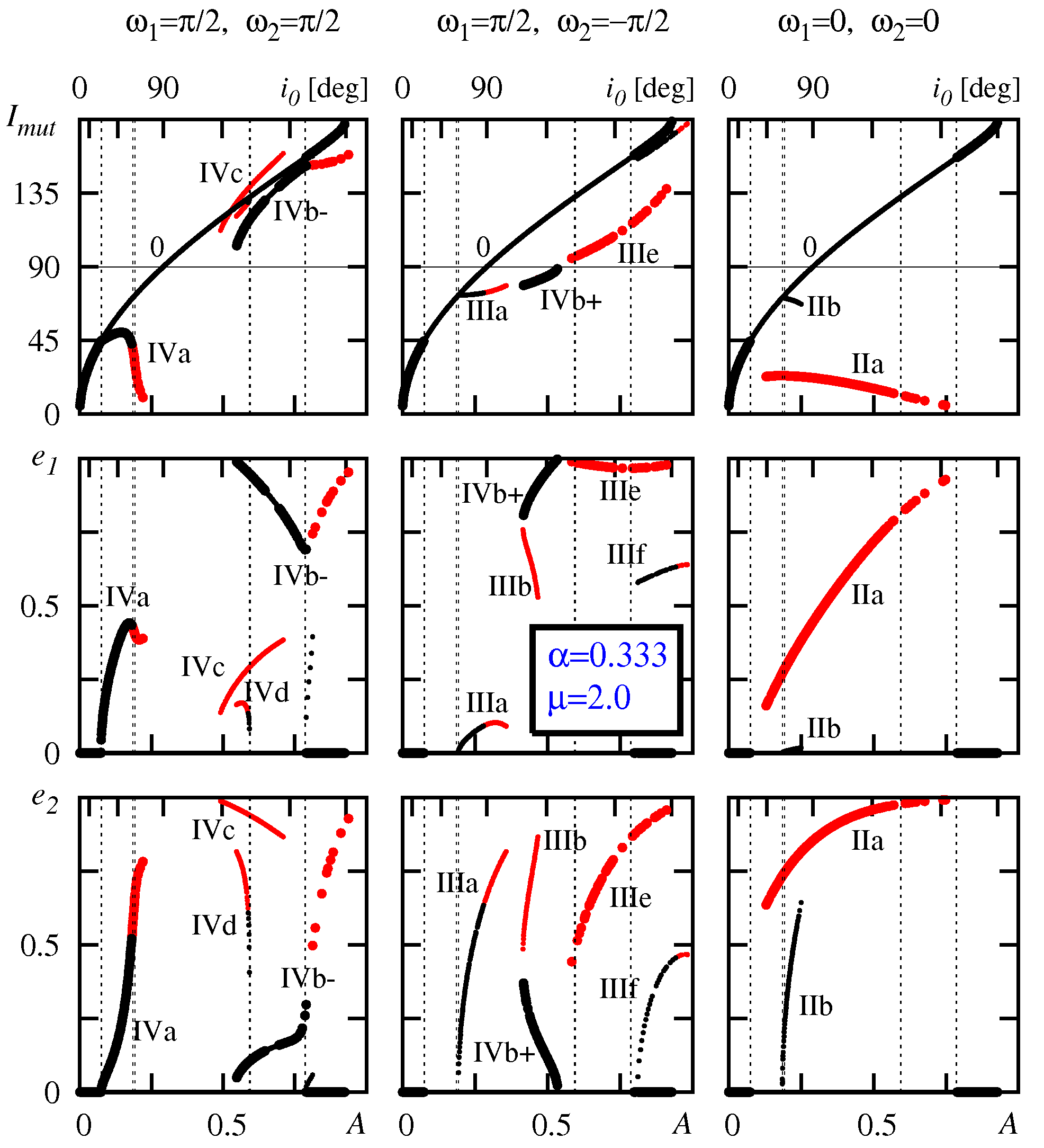
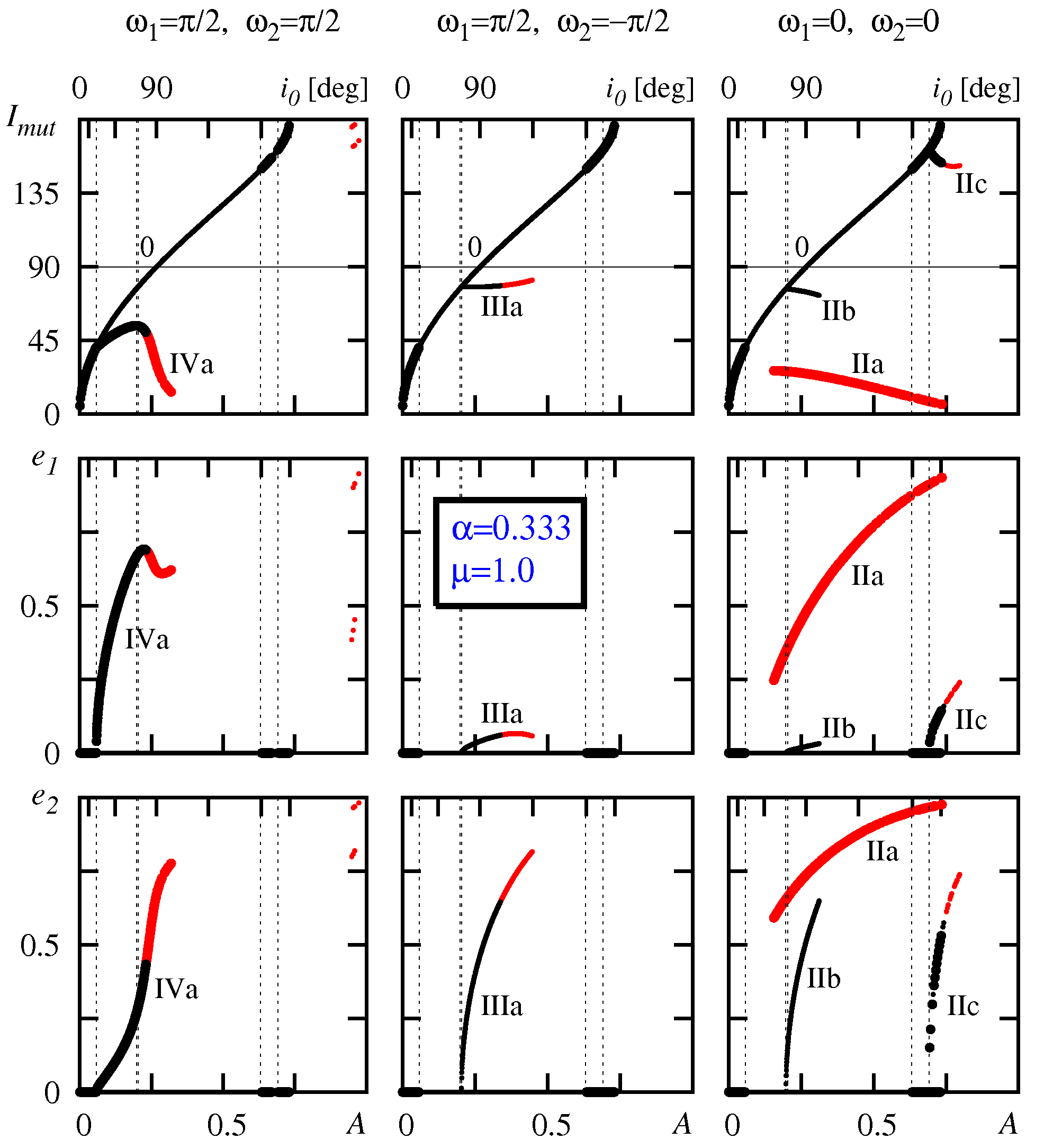
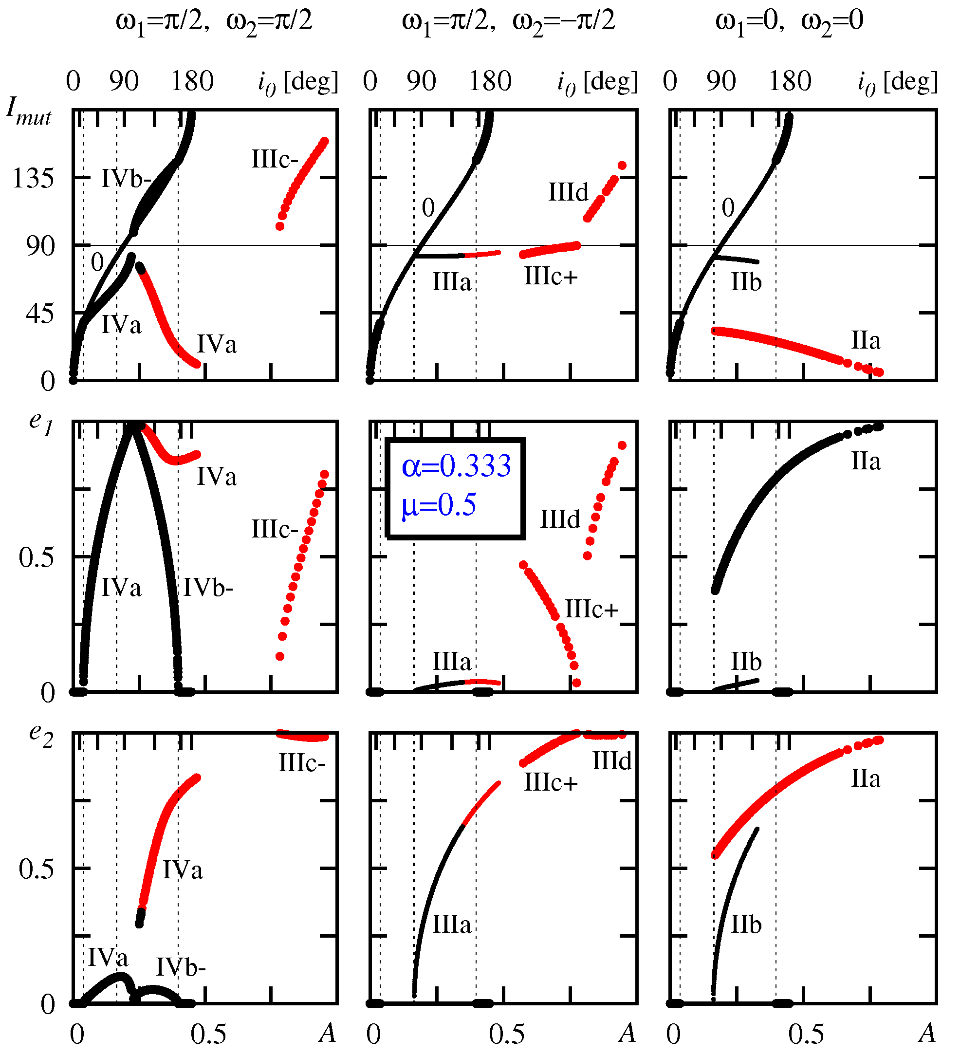
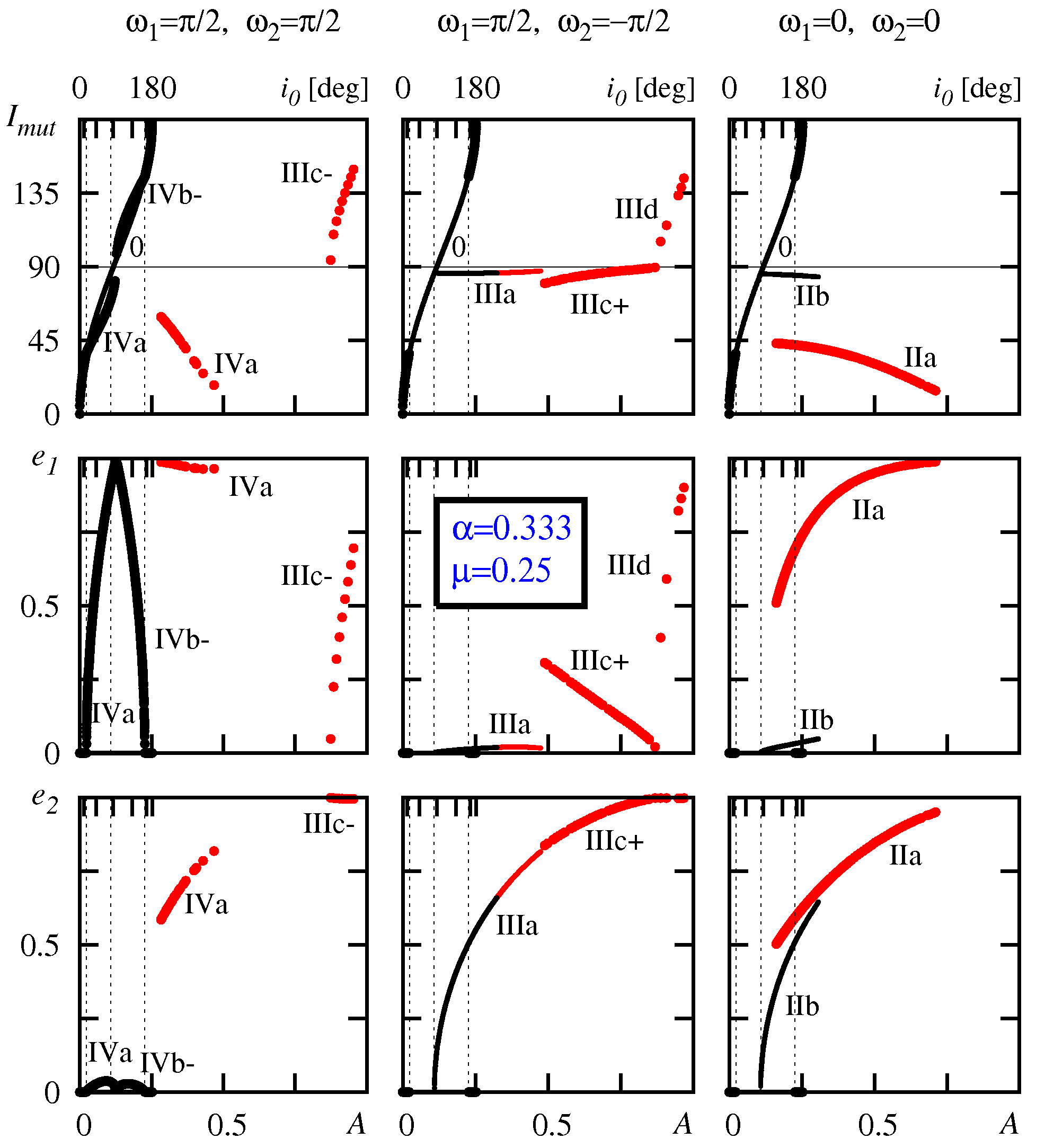
Figure 14: Families of stationary solutions obtained for $\alpha=0.333$ and the following mass ratios: $\mu=2.0$ – the top left-hand plots, $\mu=1.0$ – the top right-hand plot, $\mu=0.5$ – the bottom left-hand, and $\mu=0.25$ – the bottom right-hand plots. Large filled circle are for Lyapunov stable (or linearly stable) equilibria, smaller filled circles are for unstable equilibria, and red filled circles are for solutions found in regions, where the power series of ${\cal H}_{\mbox{\scriptsize sec}}$ in $\alpha$ would diverge. The stationary solutions are classified according with the quadrant of the $\cal S$-plane, in which they appear, hence the columns in each sub-group of diagrams [for fixed $(\alpha,\mu$) written in the legend] are for the following $(\omega_{1},\omega_{2})$-pairs: $(\pi/2,\pi/2)$ – the left column, $(\pi/2,-\pi/2)$ – the middle column, and $(0,0)$ – the right column. Each sub-group of stability diagrams has panels for the mutual inclination (the top row), and for the eccentricities (the middle and the bottom rows, respectively). The $x$-axis of each diagram is labeled by ${\mathcal{\cal A}}$ and $i_{0}$. Particular families of solutions which are identified in this work are labeled with Roman numbers and appropriate Latin letters. See the text for more details.

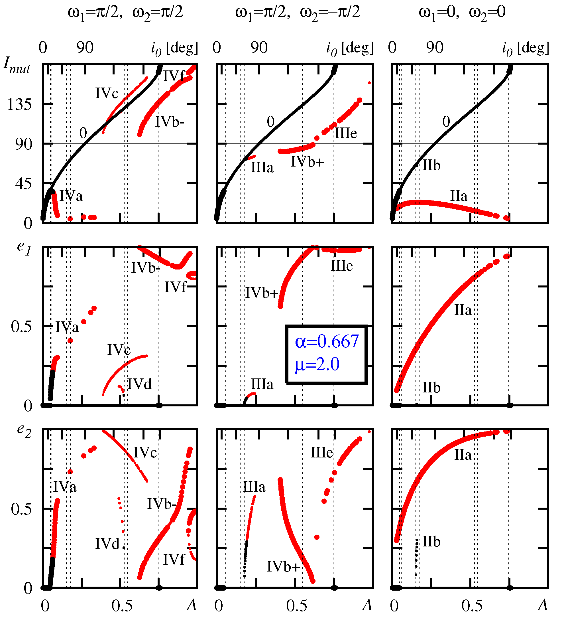
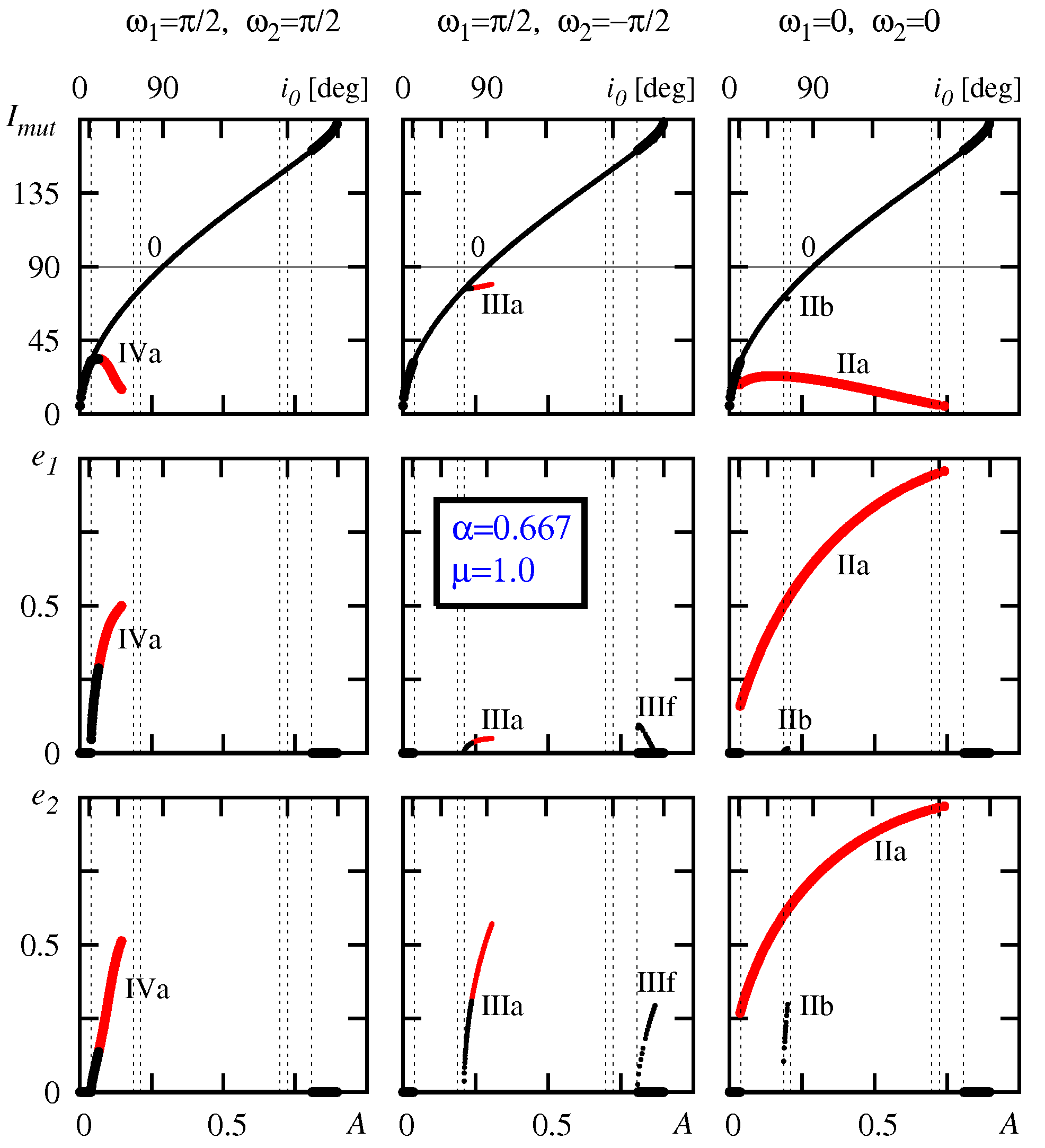
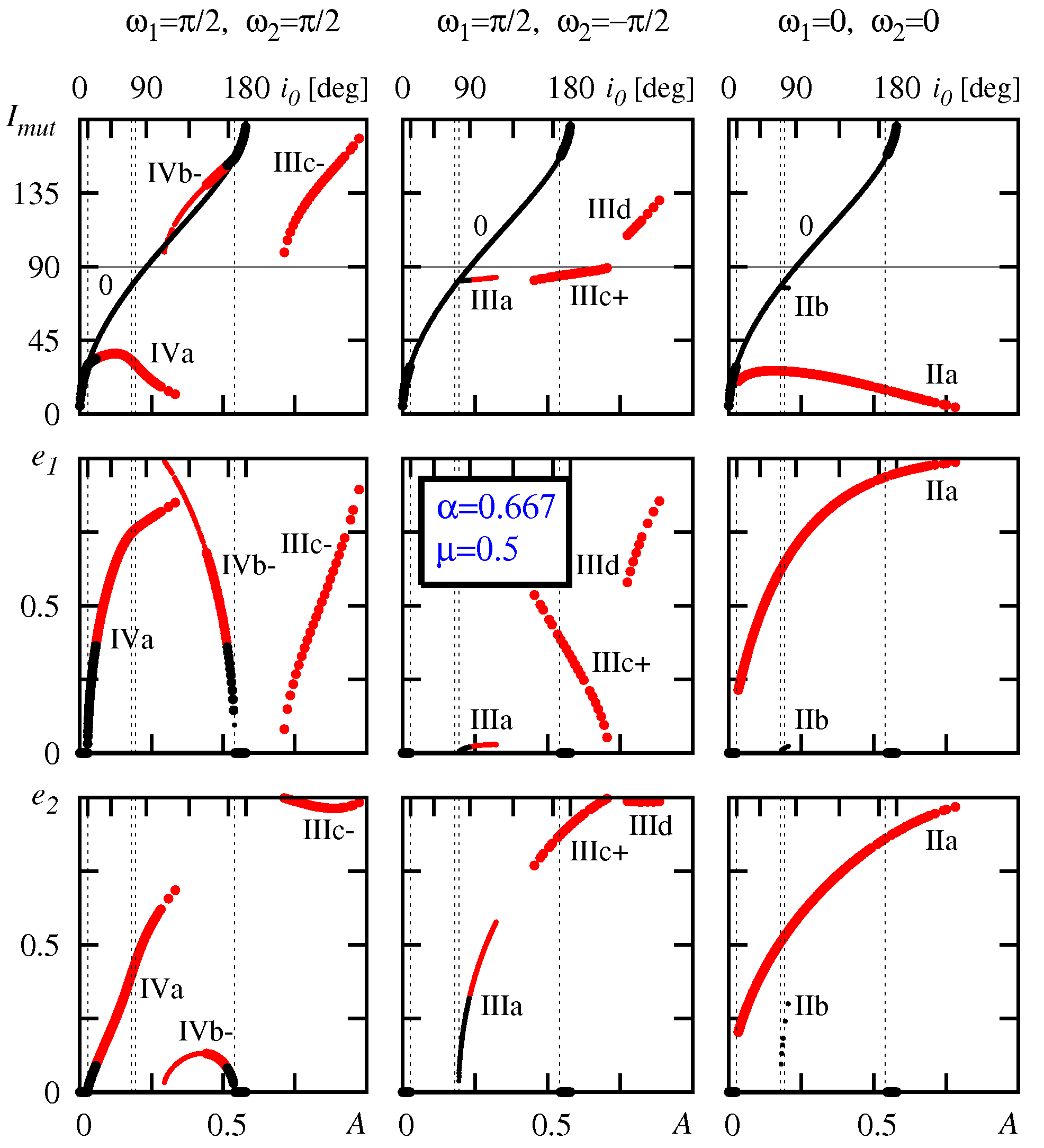
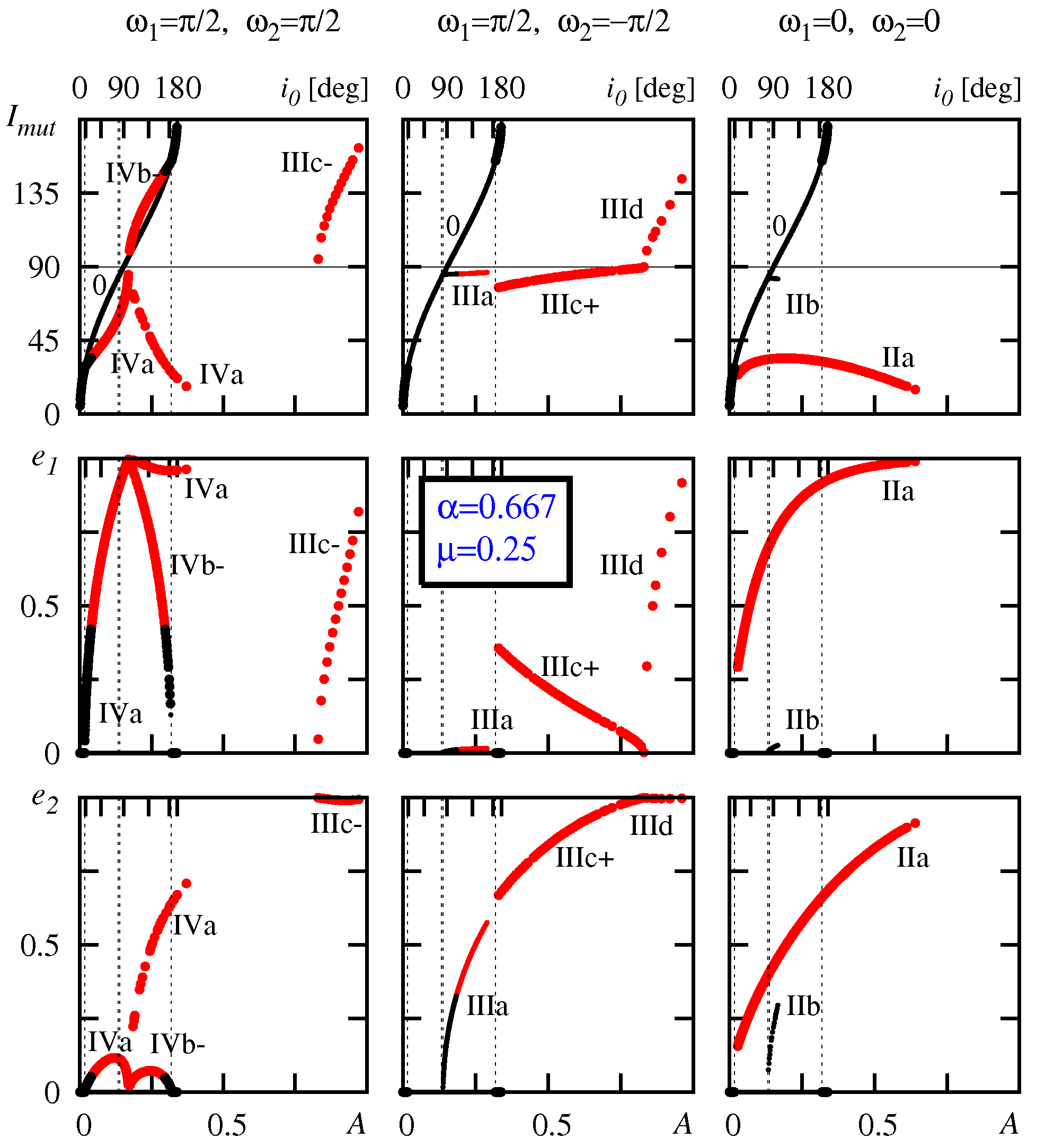
Figure 15: Families of stationary solutions obtained for $\alpha=0.667$ and the following mass ratios: $\mu=2.0$ – the top left-hand plots, $\mu=1.0$ – the top right-hand plot, $\mu=0.5$ – the bottom left-hand, and $\mu=0.25$ – the bottom right-hand plots. Large filled circle are for Lyapunov stable (or linearly stable) equilibria, smaller filled circles are for unstable equilibria, red filled circles are for solutions found in regions, where the power series of ${\cal H}_{\mbox{\scriptsize sec}}$ in $\alpha$ would diverge. The stationary solutions are classified according with the quadrant of the $\cal S$-plane, in which they appear, hence the columns in each sub-group of diagrams [for fixed $(\alpha,\mu$) written in the legend] are for the following $(\omega_{1},\omega_{2})$-pairs: $(\pi/2,\pi/2)$ – the left column, $(\pi/2,-\pi/2)$ – the middle column, and $(0,0)$ – the right column. Each sub-group of stability diagrams has panels for the mutual inclination (the top row), and for the eccentricities (the middle and the bottom rows, respectively). The $x$-axis of each diagram is labeled by ${\mathcal{\cal A}}$ and $i_{0}$. Particular families of solutions which are identified in this work are labeled with Roman numbers and appropriate Latin letters. See the text for more details.

4.2 Family Ia

Family Ia appears for a limited range of ($\alpha,\mu$) in quadrant I of the $\cal S$-plane. We detected it for $\mu\geq 1$ (more massive inner planet). This type of stationary solutions is characterized by small $e_{1}$ and a range of $e_{2}$ between 0 and a value permitted by the equation of the collision line. It emerges from a bifurcation of the zero-eccentricity solution in the range of large ${\mathcal{\cal A}}$ and is always unstable.

4.3 Families IVa, IVb-, IVb+, IIIb — the L-K resonance

We have already seen that the L-K equilibrium appears in quadrant IV of the $\cal S$-plane (family IVa) and is tightly related to family ”0” because it emerges from its “first” bifurcation on the ${\mathcal{\cal A}}$-axis. The second L-K bifurcation leads to family IVb- associated with saddles in quadrant IV and to a pair of a saddle (IVb+) and an elliptic point (family IIIb) in quadrant III. These structures are particularly well seen in the middle row of Fig. 10. Stability diagrams in Figs. 13–15 tell us that equilibria of families IVb- and IVb+ are linearly stable while solutions of family IIIb are unstable. Curiously, equilibria of family IVb+ might be identified with non-restricted case of the L-K resonance characterized by librations of $\omega_{1}$ around $\pm\pi/2$ with possible simultaneous librations of $\Delta\varpi$ around $0$ (or, equivalently, $\omega_{2}$ around $\mp\pi/2$).

To examine more closely the secular dynamics in the regime of the classic L-K resonance (family IVa), we computed the Poincaré cross sections for the secular Hamiltonian having two degrees of freedom. These cross-sections are obtained by integrating the equations of motion over a few Myr time-scale. The parameters are selected as for the HD 12661 system (see the caption to Fig. 16). The cross-section planes are chosen as follows:

$$\Sigma_{1}=\{e_{1}\cos{\Delta{\varpi}}\times e_{1}\sin{\Delta{\varpi}}\},\quad\Sigma_{2}=\{e_{1}\cos{2\omega_{1}}\times e_{1}\sin{2\omega_{1}}\}.$$

The surface of section $\Sigma_{1}$ is defined by $\omega_{1}=\pi/2$ ($d\omega_{1}/dt<0$), and the plane $\Sigma_{2}$ by $\Delta\varpi=\pi$ ($d\Delta\varpi/dt<0$), respectively. The top panels of Fig. 16 are for the $\Sigma_{1}$-plane, bottom panels of Fig. 16 are for the $\Sigma_{2}$-plane. The cross sections are computed for energy curves in the neighborhood of the L-K quasi-separatrix: panels in the left-hand column are for the initial conditions lying on the energy level within the quasi-separatrix curve encompassing the L-K resonance center, panels in the middle column are for the energy level corresponding to the quasi-separatrix curve, and the right-hand panels are for the energy level encompassing the quasi-separatrix. In the cross-sections, we can detect a few high-order secular resonances, invariant curves representing quasi-periodic orbits and relatively large regions of chaotic motions. The appearance of chaotic dynamics in the 3-D problem is the new feature as compared to the co-planar dynamics. We recall that in the later case, the averaging leads to one-degree of freedom integrable system.

Actually, the smooth invariant curves seen in the Poincaré cross sections assure us that quasi-analytic averaging makes it possible to derive very precise numerical solutions of the secular equations of motion. The Poincaré cross-sections, although obtained by complex algorithm relying on the numerical integration of the mean Hamiltonian and the equations of motion derived by numerical differentiation, make it possible to study the dynamics of the secular system in detail, and in the whole permitted range of the orbital parameters.

               

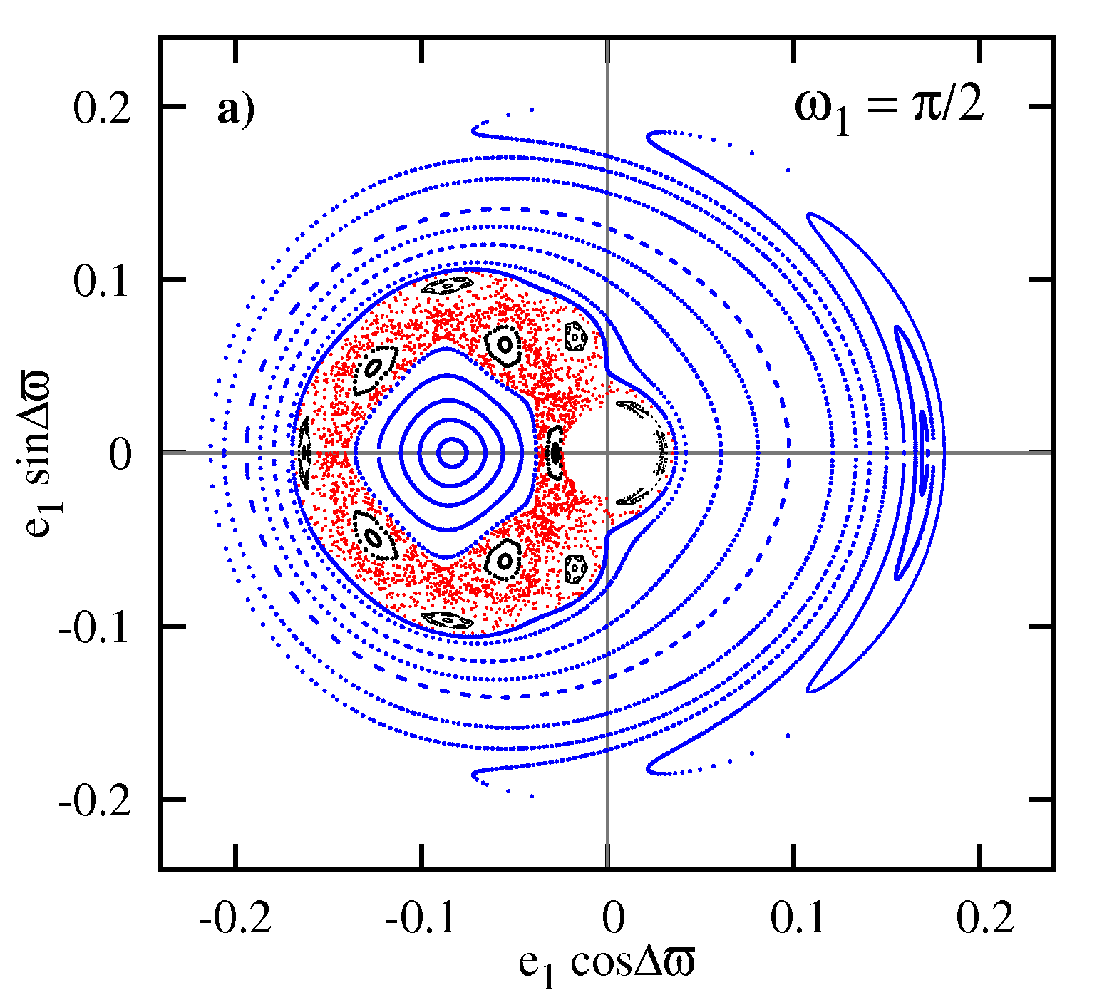
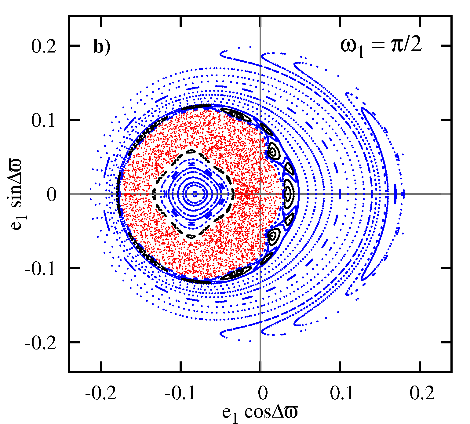
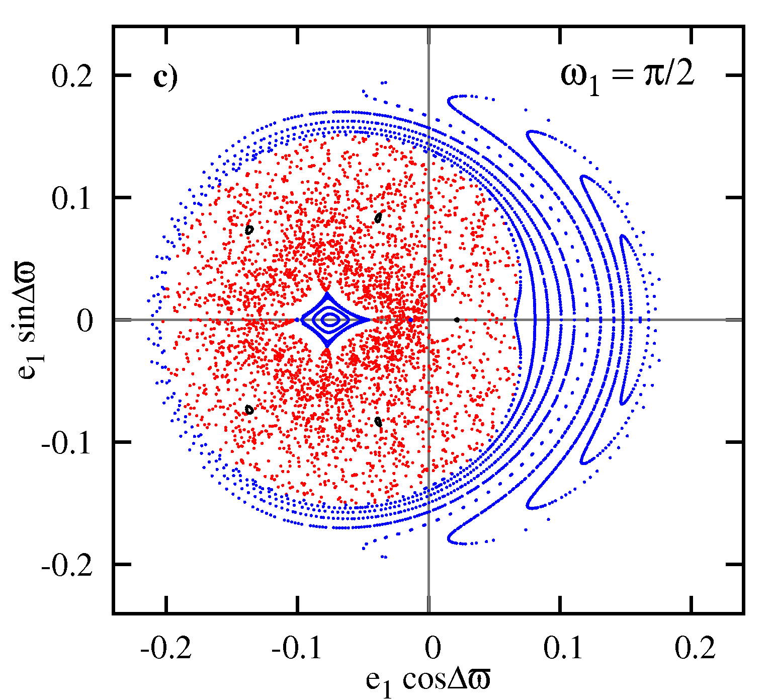
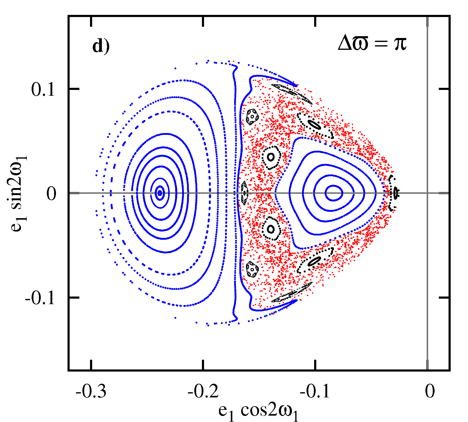
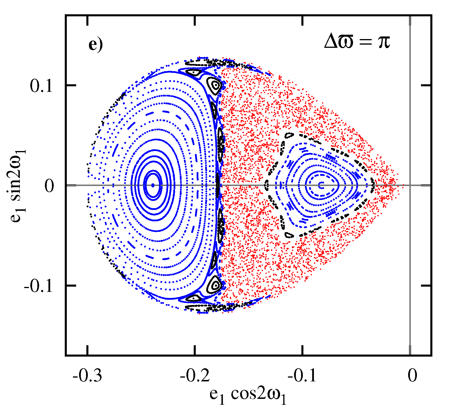
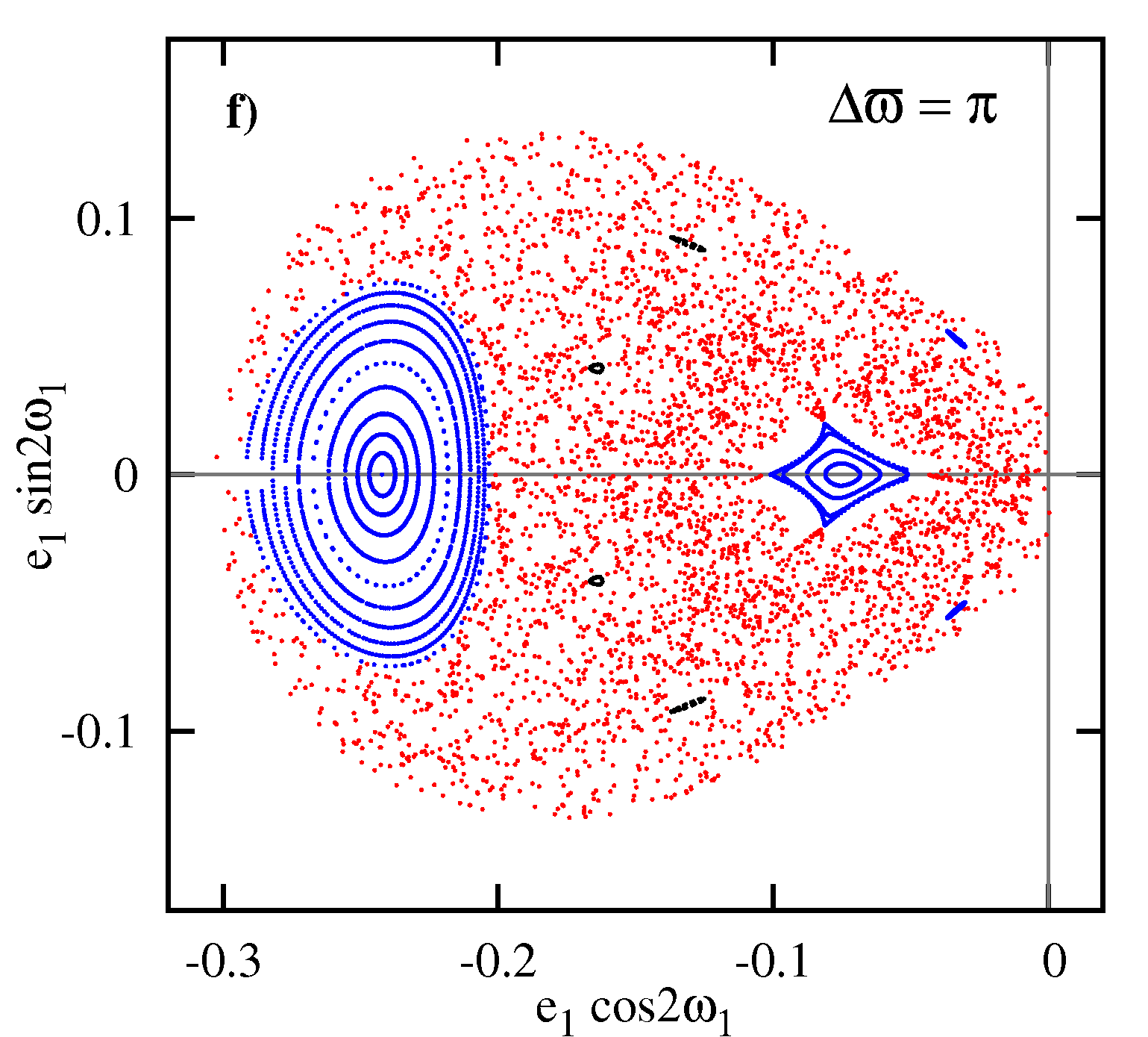
Figure 16: Poincaré cross-sections ($\omega_{1}=\pi/2$, $d\omega_{1}/dt<0$) in the top row, ($\Delta\varpi=\pi$, $d\Delta\varpi/dt<0$) in the bottom row, computed for 3D configuration of two-planet system with orbital parameters corresponding to the best–fit parameters of the HD 12661 planetary system: $m_{0}=1.07~{}\mbox{M}_{\odot}$, $m_{1}=2.3~{}\mbox{m}_{\mbox{\mbox{\scriptsize J}}}$, $m_{2}=1.57~{}\mbox{m}_{\mbox{\mbox{\scriptsize J}}}$, $a_{1}=0.83~{}\mbox{au}$, $a_{2}=2.56~{}\mbox{au}$. ${\mathcal{\cal A}}=0.085678$. The plots in columns from the left to the right are for the following secular energies: $\mathcal{E}_{a,d}=-5.106073\times 10^{-5}$, $\mathcal{E}_{b,e}=-5.106139\times 10^{-5}$, $\mathcal{E}_{c,f}=-5.106490\times 10^{-5}$ (in canonical units of 1$M_{\sun}$, 1 au, 1 yr and $k=2\pi$). These energies are chosen in the neighborhood of the Lidov-Kozai resonance. Red dots are for chaotic motions, blue dots mark quasi-periodic solutions. See the text for more details.

4.4 Families IIa and IIb

Equilibria of family IIa are very special, because they are found over the collision line of planetary orbits, hence beyond the formal limit of convergence of the expansion of ${\cal H}_{\mbox{\scriptsize sec}}$ in $\alpha$. We call them the chained stationary configurations because both secular orbits are connected like the links of a chain (see Fig. 17 for an illustration). These solutions appear at small mutual inclinations ${{\cal I}_{\mbox{\scriptsize mut}}}$. In spite of large eccentricities, the mean orbits cannot cross each other thanks to a particular spatial orientation. These equilibria are generically stable because they correspond to the maxima of ${\cal H}_{\mbox{\scriptsize sec}}$. That can be seen in the stability diagrams (Figs. 13–15). With increasing ${\mathcal{\cal A}}$, family IIa emerges close to the collision line and then “moves” towards the border of the $\cal S$-plane. Curiously, the eccentricity $e_{2}$ of equilibria IIa spans moderate and large values, and this family can be detected for all pairs of parameters analyzed in this work. The most prominent example of family IIa is shown in stability diagrams computed for $\alpha=0.667$ (see Fig. 15). We stress, that these solutions are non-resonant.

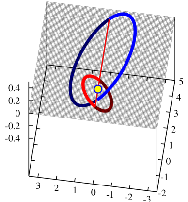
Figure 17: An example stationary configuration of family IIa computed for $a_{1}=0.83$ au, $a_{2}=2.56$ au, $e_{1}=0.325,e_{2}=0.7204$. The mutual inclination of orbits in this case is ${{\cal I}_{\mbox{\scriptsize mut}}}\sim 24^{\circ}$.

Family IIb is characterized by very small eccentricity of the inner planet and large mutual inclination of orbits (let us recall that it it may emerge for $\omega_{1}=\omega_{2}=0$). This family appears at bifurcational inclination $I_{1}^{+}$ and can be revealed by the quadrupole theory (Krasinsky, 1974). It is unstable — although it appears in the $\cal S$-plane as an elliptic point. In fact, the secular Hamiltonian is not sign definite function in its neighborhood. The linear stability analysis reveals complex eigenvalues of the linearized equations.

4.5 Families of quadrant III of the $\cal S$-plane

For small ${\mathcal{\cal A}}$, equilibria appearing in quadrant III of the $\cal S$-plane can be associated with bifurcations of the zero-family solutions. These are equilibria of family IIIa at a saddle seen in the ${\cal P}_{S}$-plane (see two last panels in the top row of Fig. 8) and appearing closely to the $e_{1}=0$ axis, and they are always unstable. Other solutions in quadrant III are associated with a bifurcation of the L-K resonance in the regime of large $e_{1}$ (families IIIb, IVb+). We note, that in our ”taxonomy”, the name of IVb+ for the saddle associated with elliptic point IIIb is justified by the fact that this point can move between quadrant IV and quadrant III (see a sequence of panels in the middle row of Fig. 10). Equilibria IIIa appear for different critical values of ${\mathcal{\cal A}}$ (or mutual inclination $i_{0}$) than solutions of family IIb. This can be particularly well seen in Fig. 15 for large $\alpha$. Moreover, the quadrupole order theory predict that these families appear for the same $i_{0}$.

In the regime of large ${\mathcal{\cal A}}$, a plethora of quadrant III solutions appears. We classify them with symbols IIIc, IIIc-, IIIc+, IIId, IIIe, IIIf (see, e.g., the right-hand panel of Fig. 3) and they are associated with large mutual inclinations of orbits and $e_{2}\sim 1$, when the energy plane become disconnected. Some of these families can be linearly stable (see the stability diagrams in Figs. 13–15). In general, the numerical continuation of these families is very difficult because they evolve close to the boundary of permitted motions in the $\cal S$-plane, and in the regime of large mutual inclinations and eccentricities. Then the numerical procedure sometimes fails, due to not precise enough determination of the second order derivatives, and that may also explain some gaps in the family curves which are present in the stability diagrams. Also problems with the continuation of these families hinder precise and proper identification of some solutions.

5 Conclusions

The semi-analytical averaging is a powerful technique helpful to reduce limitations of the analytical theories. Although it relies on purely numerical algorithms, its solid theoretical background is vital for the interpretation and understanding of the results of numerical experiments. In this work, we demonstrate that it makes it possible to study the secular dynamics of two-planet system in wide ranges of semi-major axes and masses ratio. The appropriate scaling of the problem parameters helps us to represent the phase space of the secular system globally. Assuming non-resonant configurations, and that orbits are distant enough from collision zones, the averaged system may be reduced to two degrees of freedom. Hence, to carry out the analysis, we can apply geometric tools, like the representative planes of initial conditions, Poincaré cross sections, continuations of stationary solutions with respect to parameters, which are very helpful to understand the structure of the phase space and, in turn, the long-term behavior of the planetary system.

Equilibria are the basic class of solutions which can be investigated with relatively simple tools. Our analysis reveals a number of families of stationary solutions in the 3D secular problem of two planets. To the best of our knowledge, some of them are yet unknown in the literature and are related to unusual orbital configurations. For instance, we found the so called chained stationary configuration which are non-resonant, can be found in the regime of small mutual inclinations and large eccentricities, and are located over geometric collision line of orbits. In spite of such extreme dynamical situation, these secular solutions are Lyapunov stable and exist in wide ranges of semi-major and masses ratio. Simultaneously, such orbital configurations prohibit application of analytical methods relying on power series expansion of the perturbations. The semi-analytic averaging helps to generalize analytical results obtained for low-order expansions of the secular Hamiltonian.

We obtained some interesting results regarding the Lidov-Kozai equilibrium in the non-restricted problem. We found that this resonance may be associated with librations of $\Delta\varpi$ around $\pi$ in the neighboring trajectories (not only with librations of the inner pericenter around $\pm\pi/2$). These librations are possible for relatively large ratios of semi-major axes and planetary masses. We found that the L-K resonance may also appear in the regime of large eccentricity of the inner orbit, and then it would be associated with librations of $\omega_{1}$ around $\pm\pi/2$ with simultaneous librations of $\Delta\varpi$ around $0$. The parametric evolution of the L-K resonance is related to the stability of the zero-eccentricity equilibria. There is a link between bifurcations of this family (and changes of its stability) with an appearance of new families of stationary solutions in other parts of the phase space (hence, with changes of its global topology).

Our work illustrates qualitatively different view of the 3D dynamics as compared to the coplanar configurations. It is already known (Michtchenko & Malhotra, 2004) that the non-resonant, coplanar systems of two point-mass planets fulfilling the averaging theorem and interacting through Newtonian forces are integrable. The secular dynamics of such systems are basically trivial and may be reduced to one degree of freedom. Under the same assumptions, the spatial configurations may exhibit strong chaos and extremely complex secular phenomena.

In the approximation of Newtonian, point-mass interactions, the dynamics depend on masses and semi-major axes ratios, hence our results are valid both for planetary systems with small planets, as well as for systems comprising of brown dwarfs or even sub-stellar companions. However, the dynamics of real systems may strongly depend on the magnitude of the mutual interactions. Moreover, many stable equilibria are found for large values of ${\mathcal{\cal A}}$. According to the notion of $\mathrm{AMD}$ (Laskar, 2000), in such cases the real configurations are unlikely long-term stable even close to secularly stable equilibria. In that sense, the results of stability analysis may be too optimistic. We skip a study of such effects in this work, because it would make the paper necessarily very lengthly. We should keep in mind that introduction of relativistic, tidal, and stellar quadrupole-moment perturbations, may affect the secular dynamics dramatically (Migaszewski & Goździewski, 2009b, a).

The quasi-global technique applied in this paper has been proved an efficient and effective tool for the analysis of the secular 3-D model. Nevertheless, we learned from the work that the quasi-analytical approach is not a perfect tool. Due to limitations of the numerical algorithms, the continuation of families of equilibria and analysis of their stability is particularly difficult when we reach limits of permitted motion or ${\cal H}_{\mbox{\scriptsize sec}}$ is a weakly varying function. We can also overlook some solutions. Unfortunately, that leave us sometimes with open questions.

References

- Adams & Laughlin (2003) Adams F. C., Laughlin G., 2003, Icarus, 163, 290
- Brouwer & Clemence (1961) Brouwer D., Clemence G. M., 1961, Methods of celestial mechanics. New York: Academic Press, 1961
- Brumberg (1995) Brumberg V. A., 1995, Analytical Techniques of Celestial Mechanics, Springer-Verlag Berlin Heidelberg New York
- Butler et al. (2006) Butler R. P., et. al, 2006, ApJ, 646, 505
- Fabrycky & Tremaine (2007) Fabrycky D., Tremaine S., 2007, ApJ, 669, 1298
- Ferraz-Mello et al. (2005) Ferraz-Mello S., Michtchenko T. A., Beaugé C., Callegari Jr. N., 2005, in Dvorak R., Freistetter F., Kurths J., eds., Vol. 683 of Lecture Notes in Physics, Berlin Springer Verlag, Extrasolar Planetary Systems. pp 219–+
- Ferrer & Osacar (1994) Ferrer S., Osacar C., 1994, Celestial Mechanics and Dynamical Astronomy, 58, 245
- Fischer et al. (2001) Fischer D. A., et. al, 2001, ApJ, 551, 1107
- Fischer et al. (2003) Fischer D. A., Marcy G. W., Butler R. P., Vogt S. S., Henry G. W., Pourbaix D., Walp B., Misch A. A., Wright J. T., 2003, ApJ, 586, 1394
- Ford et al. (2000) Ford E. B., Kozinsky B., Rasio F. A., 2000, ApJ, 535, 385
- Goździewski (2003a) Goździewski K., 2003a, A&A, 398, 1151
- Goździewski (2003b) Goździewski K., 2003b, Celestial Mechanics and Dynamical Astronomy, 85, 79
- Goździewski & Konacki (2004) Goździewski K., Konacki M., 2004, ApJ, 610, 1093
- Goździewski & Migaszewski (2006) Goździewski K., Migaszewski C., 2006, A&A, 449, 1219
- Innanen et al. (1997) Innanen K. A., Zheng J. Q., Mikkola S., Valtonen M. J., 1997, AJ, 113, 1915
- Ji et al. (2003) Ji J., Liu L., Kinoshita H., Zhou J., Nakai H., Li G., 2003, ApJL, 591, L57
- Khalil (2001) Khalil H. K., 2001, Nonlinear Systems. Prenitce Hall
- Kinoshita & Nakai (2007) Kinoshita H., Nakai H., 2007, Celestial Mechanics and Dynamical Astronomy, 98, 67
- Kozai (1962) Kozai Y., 1962, AJ, 67, 579
- Krasinsky (1972) Krasinsky G. A., 1972, Celestial Mechanics, 6, 60
- Krasinsky (1974) Krasinsky G. A., 1974, in Kozai Y., ed., Vol. 62 of IAU Symposium, pp 95–116
- Laskar (2000) Laskar J., 2000, Physical Review Letters, 84, 3240
- Laskar & Robutel (1995) Laskar J., Robutel P., 1995, Celestial Mechanics and Dynamical Astronomy, 62, 193
- Lee & Peale (2003) Lee M. H., Peale S. J., 2003, ApJ, 592, 1201
- Libert & Henrard (2006) Libert A.-S., Henrard J., 2006, Icarus, 183, 186
- Libert & Henrard (2007a) Libert A.-S., Henrard J., 2007a, A&A, 461, 759
- Libert & Henrard (2007b) Libert A.-S., Henrard J., 2007b, Icarus, 191, 469
- Lidov & Ziglin (1976) Lidov M. L., Ziglin S. L., 1976, Celestial Mechanics, 13, 471
- Lidov (1961) Lidov R., 1961, Izd. Akad. Nauk SSSR (1963), 1, 119
- Markeev (1978) Markeev A. P., 1978, Libration points in Celestial Mechanics and Astrodynamics. Moscow, Nauka
- Meyer & Schmidt (1986) Meyer K. R., Schmidt D. S., 1986, J. Diff. Eq., 62, 222
- Michtchenko & Ferraz-Mello (2001) Michtchenko T. A., Ferraz-Mello S., 2001, AJ, 122, 474
- Michtchenko et al. (2006) Michtchenko T. A., Ferraz-Mello S., Beaugé C., 2006, Icarus, 181, 555
- Michtchenko & Malhotra (2004) Michtchenko T. A., Malhotra R., 2004, Icarus, 168, 237
- Migaszewski & Goździewski (2008) Migaszewski C., Goździewski K., 2008, MNRAS, 388, 789
- Migaszewski & Goździewski (2009a) Migaszewski C., Goździewski K., 2009a, arXiv:0901.0102
- Migaszewski & Goździewski (2009b) Migaszewski C., Goździewski K., 2009b, MNRAS, 392, 2
- Miller & Hamilton (2002) Miller M. C., Hamilton D. P., 2002, ApJ, 576, 894
- Morbidelli (2002) Morbidelli A., 2002, Modern celestial mechanics : aspects of Solar System dynamics. Taylor & Francis, London
- Murray & Dermott (2000) Murray C. D., Dermott S. F., 2000, Solar System Dynamics. Cambridge University Press
- Press et al. (1992) Press W. H., Teukolsky S. A., Vetterling W. T., Flannery B. P., 1992, Numerical Recipes in C. The Art of Scientific Computing. Cambridge Univ. Press
- Rodríguez & Gallardo (2005) Rodríguez A., Gallardo T., 2005, ApJ, 628, 1006
- Sokolskii (1975) Sokolskii A. G., 1975, Prikladnaia Matematika i Mekhanika, 39, 366
- Thomas & Morbidelli (1996) Thomas F., Morbidelli A., 1996, Celestial Mechanics and Dynamical Astronomy, 64, 209
- Thommes & Lissauer (2003) Thommes E. W., Lissauer J. J., 2003, ApJ, 597, 566
- Veras & Armitage (2007) Veras D., Armitage P. J., 2007, ApJ, 661, 1311
- Veras & Ford (2008) Veras D., Ford E. B., 2008, ApJ, (arXiv:0811.0001)
- Wright et al. (2008) Wright J. T., Upadhyay S., Marcy G. W., Fischer D. A., Ford E. B., Johnson J. A., 2008, ApJ, (arXiv:0812.1582)