The Gravitational Shear–Intrinsic Ellipticity Correlation Functions of
Luminous Red Galaxies in Observation and in The $\Lambda$CDM Model

Abstract

We examine whether the gravitational shear–intrinsic ellipticity (GI) correlation function of the luminous red galaxies (LRGs) can be modeled with the distribution function of a misalignment angle advocated recently by Okumura et al. For this purpose, we have accurately measured the GI correlation for the LRGs in the Data Release 6 (DR6) of the Sloan Digital Sky Survey (SDSS), which confirms the results of Hirata et al. who used the DR4 data. By comparing the GI correlation functions in the simulation and in the observation, we find that the GI correlation can be modeled in the current $\Lambda$CDM model if the misalignment follows a Gaussian distribution with a zero mean and a typical misalignment angle $\sigma_{\theta}=34.9^{+1.9}_{-2.1}$ degrees. We also find a correlation between the axis ratios and intrinsic alignments of LRGs. This effect should be taken into account in theoretical modeling of the GI and intrinsic ellipticity–ellipticity correlations for weak lensing surveys.

1. Introduction

Weak gravitational lensing by large-scale structure is a promising tool to directly probe matter distribution in the universe. The main source of contaminations for weak lensing observations comes from two types of intrinsic alignments: the ellipticity correlation of source galaxies with each other [intrinsic ellipticity–ellipticity (II) correlation] and the ellipticity correlation of lense galaxies with the surrounding matter distribution [gravitational shear–intrinsic ellipticity (GI) correlation]. Investigating these intrinsic alignments is also important for galaxy formation studies.

There has been much theoretical work (e.g., Heavens et al., 2000; Croft & Metzler, 2000; Lee & Pen, 2000; Catelan et al., 2001; Jing, 2002) as well as observational work (e.g., Pen et al., 2000; Brown et al., 2002; Hirata et al., 2004; Heymans et al., 2004; Mandelbaum et al., 2006; Okumura et al., 2009) which attempted to estimate the II correlation. In Okumura et al. (2009), we have determined the II correlation of luminous red galaxies (LRGs) accurately to a large scale ($\sim 30{\hbox{$~{}h^{-1}$}{\rm~{}Mpc}}$) using the Data Release 6 of the Sloan Digital Sky Survey (SDSS DR6; York et al., 2000). From this measurement, we further gave a constraint on the misalignment angle of typically $35^{\circ}$ ($26^{\circ}$ on average) between the central giant elliptical galaxies and their host dark matter halos using the halo occupation distribution (HOD) approach (e.g., Jing et al., 1998; Zheng et al., 2008). This misalignment is found to be in agreement with the misalignment between the inner dark matter and the host halos by Faltenbacher et al. (2009) using an $N$-body simulation, though it is unknown if this is a coincidence because the light distribution of LRGs is not necessarily to be the same as the inner dark matter distribution of halos. Nevertheless, the observational constraint does provide very useful clues to understanding the contaminations on weak lensing surveys as well as to studying formation of giant ellipticals (Okumura et al., 2009).

Given the distribution of the misalignment angles, we can also predict the GI of LRGs with the surrounding dark matter distribution for current cosmological models by combining an $N$-body simulation and the HOD modeling. Such predictions can be compared with the observations of the GI such as those of Hirata et al. (2007) and Faltenbacher et al. (2009). The comparisons will further test if the distribution of the misalignment angle is correct, and will furthermore tell us how to model the GI contaminations generally for future weak lensing surveys. This approach is complementary to recently proposed statistical approaches which attempt to eliminate or minimize the GI effect in weak lensing surveys purely based on observational samples (Hirata & Seljak, 2004; King, 2005; Heymans et al., 2006; Bridle & King, 2007; Joachimi & Schneider, 2008; Zhang, 2008; Hui & Zhang, 2008). We will present such a study in this Letter.

2. SDSS Luminous Red Galaxy Sample

Our HOD model parameters used in Section 4 are from Seo et al. (2008) which is based on the fitting of Zheng et al. (2008) to the projected correlation function of LRGs of Zehavi et al. (2005). When we started the work, we tried to use the observational data of GI of Hirata et al. (2007), but later we found that the projected correlation function presented in their paper is slightly smaller (about 20 % in low-$z$ and 15 % in high-$z$ subsamples) than that in Zehavi et al. (2005). While we do not know if the samples they used are slightly different, it is apparent that the HOD parameters of Seo et al. (2008) cannot be applied to the sample of Hirata et al. (2007). Therefore, we decided to measure the GI of LRGs using the SDSS DR6 data (York et al., 2000; Eisenstein et al., 2001; Adelman-McCarthy et al., 2008). The LRG sample is the same as that used in our previous paper (Okumura et al., 2009). There are 83,773 LRGs in the redshift range $0.16<z<0.47$.

Here we need to model the radial and angular selection functions of the observational sample. We build the radial selection function by a spline fit with a Gaussian smoothing of the redshift distribution of observed LRGs. The angular selection function is constructed using the angular survey mask provided by the Value Added Galaxy Catalog (VAGC; Blanton et al., 2005). We assumed that our sample has the same survey geometry as that of the VAGC and excluded all the LRGs which are not overlapped. Then the number of LRGs is reduced to 78,758. Finally we identify 73,935 central LRGs using the criteria proposed by Reid & Spergel (2008).

We measure the projected correlation function from the LRG sample, $w_{gg}(r_{p})=\int\xi_{gg}(r_{p},\Pi)d\Pi$, where $\xi_{gg}(r_{p},\Pi)$ is the galaxy autocorrelation function as a function of separations perpendicular ($r_{p}$) and parallel ($\Pi$) to the line of sight and is measured using the Landy & Szalay (1993) estimator. Figure 1 shows the comparison of our measured $w_{gg}$ with the previous work by Zehavi et al. (2005). Very good agreement between the two studies confirmed that our selection functions work well on the scales of interests in this work.

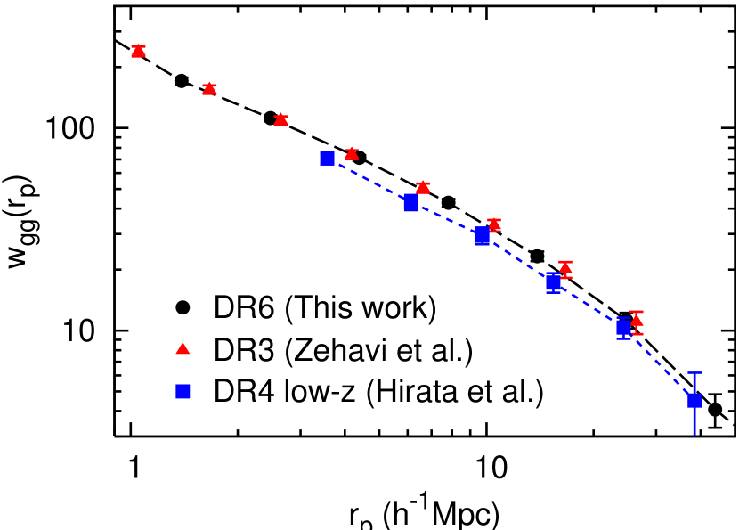
Figure 1.— Projected galaxy-galaxy correlation function for the LRG sample at $0.16<z<0.36$. For comparison, the data of Zehavi et al. (2005) and Hirata et al. (2007) are also plotted.
 

To measure the GI function of LRGs, we also need information on their shapes. The ellipticity of galaxies is determined by the SDSS photometric pipeline called photo and defined as the ellipticity of the 25 mag arcsec^-2 isophote in the $r$ band (Stoughton et al., 2002). The point-spread function has been corrected when measuring the shapes (Lupton et al., 2001). The components of the ellipticity are defined as

$$\left(\begin{array}[]{c}e_{+}\\ e_{\times}\end{array}\right)=\frac{1-q^{2}}{1+q^{2}}\left(\begin{array}[]{c}\cos{2\beta}\\ \sin{2\beta}\end{array}\right),$$ (5)

where $q$ is the ratio of minor and major axes and $\beta$ is the position angle of the ellipticity from the north celestial pole to east.

3. Gravitational Shear–Intrinsic Ellipticity Correlation of LRGs

To estimate the GI correlation, we adopt the formalism developed by Mandelbaum et al. (2006) and Hirata et al. (2007). The generalized Landy & Szalay (1993) estimator is used for estimating the GI correlation function,

$$\xi_{g+}(r_{p},\Pi)=\frac{S_{+}(D-R)}{RR}$$ (6)

where $RR$ is the normalized counts of random–random pairs in a particular bin in the space of $(r_{p},\Pi)$. $S_{+}D$ is the sum over all pairs of the $+$ component of shear in $(r_{p},\Pi)$,

$$S_{+}D=\sum_{i\neq j|r_{p},\Pi}\frac{e_{+}(j|i)}{2{\cal R}},$$ (7)

where the ellipticity component of $j$th LRG, $e_{+}(j|i)$, is redefined relative to the direction to the $i$th LRG and thus corresponds to the elongation along the direction, and ${\cal R}=1-\sigma_{\rm SN}^{2}=1-\langle e_{+}^{2}\rangle$ is the shear responsivity (e.g., Bernstein & Jarvis, 2002) and ${\cal R}\approx 0.947$ for our LRG sample. $S_{+}R$ is calculated likewise using a catalog of randomly distributed points in the survey region. Finally the projected GI correlation function is obtained by doing the projection along the radial direction,

$$w_{g+}(r_{p})=\int^{\Pi_{\rm max}}_{-\Pi_{\rm max}}\xi_{g+}(r_{p},\Pi)d\Pi.$$ (8)

We adopt $\Pi_{\rm max}=80{\hbox{$~{}h^{-1}$}{\rm~{}Mpc}}$, but changing $\Pi_{\rm max}$ from 60 to $100{\hbox{$~{}h^{-1}$}{\rm~{}Mpc}}$ does not significantly change $w_{g+}(r_{p})$ for $r_{p}<100{\hbox{$~{}h^{-1}$}{\rm~{}Mpc}}$. Positive $w_{g+}(r_{p})$ means that the major axes of LRGs tend to point toward overdensities at a transverse scale $r_{p}$. $w_{g+}$ is related to the density–intrinsic ellipticity correlation function $w_{\delta+}$ through the galaxy bias $b_{g}$ as $w_{g+}=b_{g}w_{\delta+}$ on large scales (Mandelbaum et al., 2006; Hirata et al., 2007, see also Section 5). $w_{g\times}(r_{p})$ is also calculated in the same way and used for a test of systematics because $w_{g\times}(r_{p})$ should be zero on all scales.

The resulting GI correlation functions for the observed central LRGs are shown in Figure 2. The error bars represent $1\sigma$ errors estimated from 93 jackknifed realizations. Here the axis ratio $q$ in equation (5) is set to be zero. This is equivalent to the assumption that a galaxy is a line along its major axis. In this case the shear responsivity becomes ${\cal R}=1-\langle\cos^{2}{2\beta}\rangle=0.5$. Clear detection of the GI correlation $w_{g+}$ can be seen up to large scales. Note that when our result is compared with the previous work of Hirata et al. (2007), the difference of the $q$ factor and thus of ${\cal R}$ must be taken into account. The prescription of $q=0$ and its relationship with that of $q>0$ will be discussed in Section 4.3. From the plots of $w_{g\times}$ in Figure 2 we confirm that all the values are consistent with zero at the $2\sigma$ confidence level. We thus discuss the GI correlation only in terms of $w_{g+}$ in the following analysis.

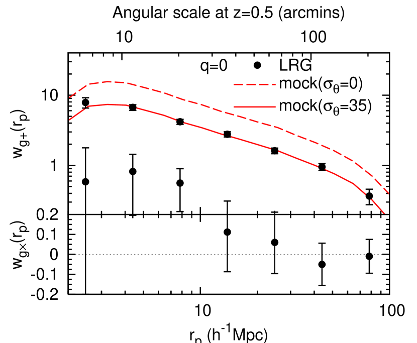
Figure 2.— Projected GI correlation functions from the SDSS central LRGs, $w_{g+}(r_{p})$ and $w_{g\times}(r_{p})$. The dashed and solid lines are respectively the model predictions for $w_{g+}$ obtained from the mock LRGs with $\sigma_{\theta}=0^{\circ}$ and $35^{\circ}$. Mixed logarithmic and linear scalings are used for the vertical axis. The horizontal axis at the top shows the corresponding angular scale when the transverse separations are located at $z=0.5$.
 

4. Comparison to Model Predictions

4.1. Modeled Gravitational Shear–Intrinsic Ellipticity Correlation Function

To make model predictions for the GI correlation, we follow the same methodology as in Okumura et al. (2009). We use a halo catalog constructed from a high-resolution cosmological simulation with $1024^{3}$ particles in a cubic box of side $1200{\hbox{$~{}h^{-1}$}{\rm~{}Mpc}}$ (Jing et al., 2007). Central galaxies are assigned to the simulated halos using the best-fit HOD parameters for LRGs found by Seo et al. (2008)(see also Zheng et al., 2008). The resulting fraction of mock central LRGs is 93.7% and we use only the centrals in order to compare with our observation.

We consider halos to have triaxial shapes (Jing & Suto, 2002). The two components of the ellipticity of each halo are estimated from the second moments of the projected mass distribution (e.g., Croft & Metzler, 2000)

$$\left(\begin{array}[]{c}e_{+}\\ e_{\times}\end{array}\right)=\frac{1}{I_{xx}+I_{yy}}\left(\begin{array}[]{c}I_{xx}-I_{yy}\\ 2I_{xy}\end{array}\right),$$ (9)

where $I_{ij}=\frac{1}{N}\sum^{N}x_{i}x_{j}$ and $N$ is the number of particles in a halo. Then the GI correlation function of halos is measured in the same way as that of LRGs, where the value of $q$ is assumed to be zero again and thus ${\cal R}=0.5$.

First we assume that all central galaxies are completely aligned with their parent dark matter halos. The GI correlation function of central galaxies is then calculated and shown in Figure 2. In order to refine the statistics, we averaged over seven mock samples with different random seeds for assigning LRGs to dark halos. Interestingly, the GI correlation function of the mock LRGs, when they are assumed to be aligned completely with their host halos, has the same shape as but is about twice as high as the observation. Similar results were shown for the II correlation (Okumura et al., 2009).

4.2. Constraints on Misalignment

In this subsection, we consider the case in which the major axis of each central galaxy is misaligned with that of its host halo and give a constraint on the misalignment angle by comparing the observed GI correlation function $w_{g+}$ with its model prediction. Following Okumura et al. (2009) we assume that the misalignment angle $\theta$ between the major axes of central LRGs and their host halos follows a Gaussian function with a zero mean and a width $\sigma_{\theta}$, where $\sigma_{\theta}$ is the typical misalignment angle. We artificially assign misalignment to the position angle of each mock central LRG relative to its host halo according to the Gaussian function. For each chosen value of $\sigma_{\theta}$ and each LRG mock sample, we generate nine misaligned LRG samples by choosing different random seeds. Our model prediction for each $\sigma_{\theta}$ is thus calculated by averaging over $7\times 9=63$ misaligned samples.

In comparing the observational data with the model prediction, $\chi^{2}$ statistics are calculated in the range of $20^{\circ}<\sigma_{\theta}<50^{\circ}$. In this analysis we use the seven data points of $w_{g+}(r_{p})$ shown in Figure 2, while there is one free parameter, $\sigma_{\theta}$; thus the degree of freedom is 6. The covariance matrix estimated using 93 jackknifed subsamples is used for the calculation of $\chi^{2}$.

The fits of the observed GI correlation function $w_{g+}$ to the model prediction give a tight constraint on the misalignment parameter, $\sigma_{\theta}=34.9^{+1.9}_{-2.1}$ degrees (68% confidence level), which corresponds to a mean misalignment angle of $26^{\circ}.9$. This is in very good agreement with our previous work on the II correlation which gave $\sigma_{\theta}=35.4^{+4.0}_{-3.3}$ degrees. The constraint from the GI correlation is tighter than that from the II correlation because the GI correlation is better determined. The model prediction of $w_{g+}$ with $\sigma_{\theta}=35^{\circ}$ is shown in Figure 2.

4.3. Correlation of the LRG shape and its orientation

The misalignment parameter was constrained with the assumption of $q=0$, i.e., we considered the orientation of the LRGs relative to their spatial distribution only. If there is no correlation between the shape of the LRGs and their orientation, we can use the misalignment angle distribution to model the GI of LRGs even when the shape is included (i.e., GI in weak lensing studies; Hirata et al., 2007). In order to see if this correlation exists, we define a normalized GI correlation function $\bar{w}_{g+}$ as

$$\bar{w}_{g+}(r_{p};q)=\left\langle{\frac{1-q^{2}}{1+q^{2}}}\right\rangle^{-1}w_{g+}(r_{p};q),$$ (10)

where $\left\langle{\frac{1-q^{2}}{1+q^{2}}}\right\rangle$ is the value averaged over all objects in the sample (it is $0.29$ for observed LRGs and $0.42$ for mock host halos of LRGs), and $w_{g+}(r_{p};q)$ is the same as equation (8) except the $q$ dependence is included. If there is no correlation between axis ratios and orientations, we expect $\bar{w}_{g+}(r_{p};q=q_{\rm LRG})={w}_{g+}(r_{p};q=0)$ for observed LRGs and $\bar{w}_{g+}(r_{p};q=q_{\rm mock})={w}_{g+}(r_{p};q=0)$ for halos. Here we neglect the factor of the shear responsivity, $1/2{\cal R}$, so equation (10) just corresponds to the replacement of $1/2{\cal R}$ by $\left\langle{\frac{1-q^{2}}{1+q^{2}}}\right\rangle^{-1}$ in equation (7).

In Figure 3 we show $\bar{w}_{g+}(r_{p};0)$ of the observed LRGs and mock LRGs with $\sigma_{\theta}=35^{\circ}$, which are the same data as those in Figure 2 because $\bar{w}_{g+}(r_{p};0)=w_{g+}(r_{p};0)$. Next we calculate $\bar{w}_{g+}(r_{p};q_{\rm mock})$ for the mock LRGs with $q_{\rm mock}$ determined from the dark matter distribution within the host halos, which is shown as the dashed line in Figure 3. These results indicate that there exists a correlation between the shape and orientation of the dark matter halos, and this correlation leads to an increase of $\sim 15\%$ in the normalized GI correlation. If the shapes of the halos were uncorrelated with their orientations, we expect that this $\bar{w}_{g+}(r_{p};q_{\rm mock})$ would be equal to $\bar{w}_{g+}(r_{p};0)$. This is indeed confirmed in the figure, where the dotted line, the correlation when the values $q_{\rm mock}$ (not the orientation) of host halos are shuffled randomly, is completely overlapped with the solid line. Almost the same amount of increase is seen for the GIs of the observed LRGs, as shown by the squares and the circles in the figure, which implies that there is a correlation of the shapes and orientation in the observation.

This correlation should be taken into account when one models the GI and II effects in theory by using the distribution function of the misalignment angle. It should also be considered if $w_{g+}(r_{p};q=q_{\rm LRG})$ is used to constrain the distribution function of the misalignment angle. If the correlation is neglected, the misalignment angle could be slightly underestimated. This is the reason why only the orientation of the LRGs are used in Okumura et al. (2009) and in the current work to constrain the misalignment angle.

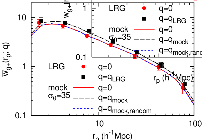
Figure 3.— Normalized GI correlation functions $\bar{w}_{g+}(r_{p};q)$. All the lines are the model predictions with $\sigma_{\theta}=35^{\circ}$. The dotted blue line is the one with $q_{\rm mock}$ shuffled randomly. The circles/squares have been respectively offset in the horizontally negative/positive direction for clarity.
 

5. Discussion

In this Letter, we examined whether the GI correlation of LRGs can be modeled with the distribution function of misalignment angle advocated by Okumura et al. (2009) based on the II correlation. For this purpose, we have accurately measured the GI correlation for the LRGs in the SDSS DR6, which also confirms the results of Hirata et al. (2007) who used the DR4 data. By comparing the GI correlations in the simulation and in the observation, we found that the GI correlation can be modeled in the current $\Lambda$CDM model, if the misalignment follows a Gaussian distribution with a zero mean and a typical misalignment angle $\sigma_{\theta}=34.9^{+1.9}_{-2.1}$ degrees. This constraint on $\sigma_{\theta}$ is in excellent agreement with the previous work, $\sigma_{\theta}=35.4^{+4.0}_{-3.3}$ degrees, based on the II correlation. The constraint on $\sigma_{\theta}$ is tighter in this Letter, because the GI correlation is better determined than the II correlation in the observation. Furthermore, the good agreement of the observed and theoretical GI functions further lends nontrivial support for the $\Lambda$CDM scenarios and for the distribution function of the misalignment angle.

We have found a correlation between the axis ratios and intrinsic alignments of LRGs. If the correlation is neglected, one would underestimate the GI correlation (in the case of $q\neq 0$) by $\sim 15\%$ if the shape $q$ and orientation $\theta$ of the LRGs are randomly chosen from their distribution functions. This effect should be taken into account in theoretical modeling of the GI and II correlations for weak lensing surveys.

These results have profound implications both for future weak lensing surveys and for studying the formation of giant elliptical galaxies. For weak lensing surveys, the relevant quantity is the correlation function between the mass overdensity and the intrinsic ellipticity, $w_{\delta+}$. As Mandelbaum et al. (2006) and Hirata et al. (2007) reasoned, these two quantities are simply related through the galaxy bias as $w_{g+}=b_{g}w_{\delta+}$. We can also measure $w_{\delta+}$ directly in our simulation. Our result supports that $b_{g}$ in this simple relation is about 2 for all the scales explored here and for our chosen $\Lambda$CDM model.

References

- Adelman-McCarthy et al. (2008) Adelman-McCarthy, J. et al. 2008, ApJS, 175, 297
- Bernstein & Jarvis (2002) Bernstein, G. M., & Jarvis, M. 2002, AJ, 123, 583
- Blanton et al. (2005) Blanton, M. R., et al. 2005, AJ, 129, 2562
- Bridle & King (2007) Bridle, S., & King, L. 2007, New J. Phys., 9, 444
- Brown et al. (2002) Brown, M. L., Taylor, A. N., Hambly, N. C., & Dye, S. 2002, MNRAS, 333, 501
- Catelan et al. (2001) Catelan, P., Kamionkowski, M., & Blandford, R. D. 2001, MNRAS, 320, L7
- Croft & Metzler (2000) Croft, R. A. C. & Metzler, C. A. 2000, ApJ, 545, 561
- Eisenstein et al. (2001) Eisenstein, D. J., et al. 2001, AJ, 122, 2267
- Faltenbacher et al. (2009) Faltenbacher, A., Li, C., White, S. D. M., Jing, Y. P., Mao, S., & Wang, J. 2009, RAA, 9, 41
- Heavens et al. (2000) Heavens, A., Refregier, A., & Heymans, C. 2000, MNRAS, 319, 649
- Heymans et al. (2004) Heymans, C., Brown, M., Heavens, A., Meisenheimer, K., Taylor, A., & Wolf, C. 2004, MNRAS, 347, 895
- Heymans et al. (2006) Heymans, C., White, M., Heavens, A., Vale, C., & Waerbeke, L. V. 2006, MNRAS, 371, 750
- Hirata et al. (2007) Hirata, C. M., Mandelbaum, R., Ishak, M., Seljak, U., Nichol, R., Pimbblet, K. A., Ross, N. P., & Wake, D. 2007, MNRAS, 381, 1197
- Hirata & Seljak (2004) Hirata, C. M., & Seljak, U. 2004, Phys. Rev. D, 70, 063526
- Hirata et al. (2004) Hirata, C. M., et al. 2004, MNRAS, 353, 529
- Hui & Zhang (2008) Hui, L., & Zhang, J. 2008, ApJ, 688, 742
- Jing (2002) Jing, Y. P. 2002, MNRAS, 335, L89
- Jing et al. (1998) Jing, Y. P., Mo, H. J., & Boerner, G. 1998, ApJ, 494, 1
- Jing & Suto (2002) Jing, Y. P., & Suto, Y. 2002, ApJ, 574, 538
- Jing et al. (2007) Jing, Y. P., Suto, Y., & Mo, H. J. 2007, ApJ, 657, 664
- Joachimi & Schneider (2008) Joachimi, B., & Schneider, P. 2008, A&A, 488, 829
- King (2005) King, L. J. 2005, A&A, 441, 47
- Landy & Szalay (1993) Landy, S. D., & Szalay, A. D. 1993, ApJ, 412, 64
- Lee & Pen (2000) Lee, J., & Pen, U. L. 2000, ApJ, 532, L5
- Lupton et al. (2001) Lupton, R. H., Gunn, J. E., Ivezic, Z., Knapp, G. R., Kent, S., & Yasuda, N. 2001, in ASP Conf. Ser. 238, Astronomical Data Analysis Software and Systems X, ed. F. R. Harnden, Jr., F. A. Primini, and H. E. Payne (san Francisco, CA: ASP), 268 (arXiv:astro-ph/0101420)
- Mandelbaum et al. (2006) Mandelbaum, R., Hirata, C. M., Ishak, M., Seljak, U., & Brinkmann, J. 2006, MNRAS, 367, 611
- Okumura et al. (2009) Okumura, T., Jing, Y. P., & Li, C. 2009, ApJ, in press (arXiv:0809.3790)
- Pen et al. (2000) Pen, U. L., Lee, J. Seljak, U. 2000, ApJ, 543, L107
- Reid & Spergel (2008) Reid, B. A., & Spergel, D. N. 2008, arXiv:0809.4505
- Seo et al. (2008) Seo, H.-J., Eisenstein, D. J., & Zehavi, I. 2008, ApJ, 681, 998
- Stoughton et al. (2002) Stoughton, C., et al. 2002, AJ, 123, 485
- York et al. (2000) York, D. G., et al. 2000, AJ, 120, 1579
- Zehavi et al. (2005) Zehavi, I. et al. 2005, ApJ, 621, 22
- Zhang (2008) Zhang, P. 2008, arXiv:0811.0613
- Zheng et al. (2008) Zheng, Z., Zehavi, I., Eisenstein, D. J., Weinberg, D. H., & Jing, Y. P. 2008, arXiv:0809.1868