Gravity Waves from Tachyonic Preheating after Hybrid Inflation

Abstract

We study the stochastic background of gravitational waves produced from preheating in hybrid inflation models. We investigate different dynamical regimes of preheating in these models and we compute the resulting gravity wave spectra using analytical estimates and numerical simulations. We discuss the dependence of the gravity wave frequencies and amplitudes on the various potential parameters. We find that large regions of the parameter space leads to gravity waves that may be observable in upcoming interferometric experiments, including Advanced LIGO, but this generally requires very small coupling constants.

I Introduction

Gravity waves (GW) from the early universe can carry information about inflation, (p)reheating after inflation, and even about pre-inflation.

During inflation, tensor modes of the classical large scale cosmological perturbations are produced from the quantum fluctuations of gravitons starob79 . Their amplitude is proportional to the energy scale of inflation, and their spectrum extends over a wide range of wavelengths. Gravitational waves at the cosmological, long-wavelength part of the spectrum lead to B-mode polarization of the CMB anisotropy fluctuations. In high energy models of inflation (like chaotic inflation), where the ratio of the amplitudes of the tensor to scalar modes is about $r\sim 0.1$, the B-mode of anisotropies should be detectable by forthcoming CMB polarization experiments.

However, in anticipation of a null signal observation of GW from inflation, one might still be able to use GW to constrain inflationary models in ways other than just constraining the overall energy scale. There are models of inflation where the total number of inflationary e-folds $N$ exceeds the minimum required to homogenize the observable universe only by a small margin. For such models with anisotropic pre-inflationary expansion, gravity waves from pre-inflation are amplified and may contribute to the large scale CMB temperature anisotropy GKP . Observational limits on gravity waves from CMB polarization experiments also result in constraints on $N$.

If inflation occurs at lower energies (as in many hybrid inflation models), the amplitude of the resulting gravity waves would be too weak to be observed with CMB anistropies. However, GW from inflation at the short-wavelength part of the spectrum might fall in the amplitude-frequency range which accessible to future gravity wave astronomy projects such as BBO and DECIGO. These experiments could probe $r$ down to the level $r\sim 10^{-6}$.

Gravity waves may also carry unique information about the post-inflationary dynamics, in particular the inflaton decay and the subsequent evolution of its decay products towards thermal equilibrium. Often this process starts with preheating, a violent non-perturbative restructuring of the field configurations shortly after inflation. Preheating leads to large, non-linear field inhomogeneities which necessarily generate a classical GW background. This mechanism of GW production is complementary to the production of GW from vacuum fluctuations during inflation. In our previous paper DBFKU we developed a machinery for analytic and numerical calculations of GW production in preheating models. There are several other papers on the subject that we will discuss below. It is also worth mentioning that the techniques used to study GW from preheating have parallels in calculations of GW from phase transitions / hydrodynamical turbulence, see e.g. transitions and references therein. In DBFKU we developed applications of our methods to the example of preheating after chaotic inflation. The parameters of these large-field models are fixed by CMB normalization, which ensures that inflation must occur at high energy scales. As a result, the gravity waves produced from preheating in these models have typical frequencies of order $f\sim 10^{7}-10^{8}$ Hz, which is far beyond the observable range (see Section VI for observational constraints). As conjectured in frag , preheating after low-energy inflation may generate GW with lower frequencies $f$. One of the most popular and most studied models of inflation and preheating is hybrid inflation hybrid with tachyonic preheating tachpre . There are many hybrid inflation models, notably in the context of supergravity (see lythriotto for a review) and string theory (see stringinf for reviews). In these models, the energy scale of inflation is not fixed by CMB normalization, so it was optimistically thought that for some parameters the frequency of GW from preheating may fall into an observable range. The subject of this paper is GW production from tachyonic preheating, in particular, assessing how realistic is the range of parameters that may lead to an observable signal.

Let us briefly review the literature on the subject. The production of gravitational waves from preheating was originally studied in pregw1 for chaotic inflation, and recently by several groups in pregw2 ; frag ; pregw3 ; juan1 ; juan2 ; DBFKU ; pregw4 ; pregw5 . The first numerical methods pregw1 ; pregw2 were based on the Weinberg formalism weinberg , which, strictly speaking is applicable only for isolated sources in a Minkowski background. This may lead to significant differences in the resulting gravity wave spectra, as explained in DBFKU . In pregw3 , the gravity wave equations in an expanding universe were solved in Fourier space. Another method was used in juan1 ; juan2 , where the evolution equation for metric perturbations were solved in configuration space. In juan1 and the earlier version of juan2 the transverse-traceless radiative part of GW was not properly extracted but after discussion of the problem in DBFKU this was corrected in the second version of juan2 . Finally, in DBFKU , we developed a method based on the Green’s function solution in momentum space, to calculate, numerically and analytically, the production of gravity waves from a stochastic medium of scalar fields in an expanding universe. At present, the numerical methods of different groups pregw3 , juan2 and DBFKU seem to agree well with each other, see pregw4 ; pregw5 for a comparison of the results in a model of chaotic inflation.

Most of these papers focused on models of preheating based on parametric resonance after chaotic inflation, which leads to gravity wave signals at frequencies which are irrelevant observationally. Models of preheating after hyrbid inflation are observationally much more interesting, because they involve extra parameters and they occur at lower energy scales, and thus they may generate GW with lower frequencies. Gravity wave production after hybrid inflation was first considered in juangw , extrapolating the results of pregw1 , assuming that preheating occurs through parametric resonance. However, we know since tachpre that preheating after hybrid inflation occurs in the qualitatively different regime of tachyonic amplification due to the dynamical symmetry breaking, when the fields roll towards the minimum through the region where their effective mass is negative – a process called tachyonic preheating. It completes in one or very few oscillations of the fields and is very different from parametric resonance.

Before further discussion on GW, we have to comment about specific challenges for numerical simulations of tachyonic preheating in hybrid inflation models with several parameters . These parameters include the self-coupling $\lambda$ of the symmetry breaking fields and their coupling $g^{2}$ to the inflaton. The scales of the preheating dynamics can be significantly different depending on the combination $g^{2}/\lambda$ (roughly speaking, the ratio of effective masses around the local maximum and minimum of the potential). Therefore, care should be taken to incorporate both scales in the simulations. An additional subtlety is related to the initial conditions for the fields around the bifurcation point, namely, relatively high or low inflaton velocity, which results in qualitatively different initial regimes – quantum diffusion or classical fast or slow rolls around the bifurcation point, see tachpre for details. The case with higher initial velocity is easier to model numerically.

The production of gravitational waves properly from tachyonic preheating was first investigated in juan1 ; juan2 , for a specific region of the parameter space ($g^{2}\sim\lambda\sim 1$ and significant velocity of the inflaton at the bifurcation point), where the dynamical scales are of the same order. The resulting gravity wave spectra were located at frequencies too high to be observable, as in chaotic inflation models. Refs. juan1 ; juan2 also displayed a conjecture for a low frequency spectrum, but the dependence on the parameters was not studied, so it remains unclear which model, if any, could lead to an observable signal. In frag , it was conjectured that the peak frequency and amplitude of the gravity wave spectrum depends in a relatively simple way on the typical scale amplified during preheating, which is usually a known function of the parameters. In DBFKU we verified this conjecture numerically for a model of chaotic inflation, and used it to estimate analytically the peak of the gravity wave spectrum produced in two different models of preheating after hybrid inflation. In particular, we noticed that models with low velocity of the inflaton at the critical point are observationally more promising, but it is also more challeging to model this case with numerical simulations, as noted above.

In the present paper, we investigate in detail gravity waves produced from preheating after hybrid inflation, focusing in particular on their dependence on various model parameters such as $g^{2}/\lambda$ and the field velocities around the bifurcation point. We study GW production in several qualitatively different settings of tachyonic preheating, some of which, including the most interesting cases, were completely missed in the literature. We use a combination of analytical estimates and improved numerical simulations to compute the resulting gravity wave spectra and to identify the regions of the parameter space which may be relevant for upcoming gravity wave experiments.

The rest of the paper is organized as follows. In Section II, we briefly review the hybrid inflation models that we will consider. In Section III, we identify three qualitatively different dynamical regimes of preheating in these models and we make analytical estimates of the resulting gravity wave spectra. In Section IV we describe and advance further our numerical method for calculating gravity wave production from preheating. We apply this method to preheating after hybrid inflation in Section V and we study the dependence of the gravity wave amplitudes and frequencies on the parameters of the model. We then discuss which regions of the parameter space may lead to a detectable signal. Finally, we discuss the implications of our results and directions for future work. Some details of our numerical calculations are given in the appendices.

II Parameters of the Hybrid Inflation Model

We will consider simple hybrid inflation models with the potential

$$V={1\over 4}\lambda\left(\sigma^{2}-v^{2}\right)^{2}+{1\over 2}g^{2}\phi^{2}\sigma^{2}+V_{inf}(\phi).$$ (1)

The Higgs field $\sigma$ may in principle be real, complex, or consisting of any number of components, but the case of a real field is ruled out because it would lead to the production of dangerous sub-horizon size domain walls. We have tried simulations with varying numbers of $\sigma$ components and found the results to be largely unaffected. The simulations shown below are for a two-component $\sigma$, for which $\sigma^{2}$ should be understood as $|\sigma|^{2}=\sigma_{1}^{2}+\sigma_{2}^{2}$ where $\sigma_{1}$ and $\sigma_{2}$ are two real scalar fields. We take the inflaton $\phi$ to be real for simplicity.

For $\phi>\phi_{c}\,$, where

$$\phi_{c}\equiv\frac{\sqrt{\lambda}}{g}\,v$$ (2)

is the critical point, the fields have positive mass squared and the potential has a valley at $\sigma=0$. Inflation occurs while $\phi$ decreases slowly in this valley due to the uplifting term $V_{inf}(\phi)$ in (1). The energy density is usually dominated by the false vacuum contribution, $V\simeq\lambda v^{4}/4$. Inflation ends either at the bifurcation point when $\phi=\phi_{c}$ or when the slow-roll conditions are violated, whichever occurs first. In both cases, when $\phi=\phi_{c}$, $\sigma$ acquires a tachyonic mass and the fields roll rapidly towards the true minimum at $\phi=0$, $\sigma=v$. During this rolling field fluctuations are exponentially excited by tachyonic preheating tachpre , thus leading to a rapid decay of the homogeneous field energy, see Fig. 1. This exponentially rapid growth of inhomogeneities is what drives the production of gravity waves in this model.

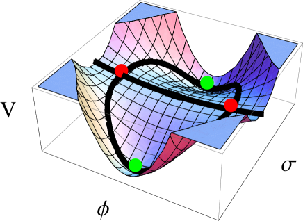
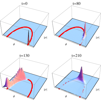
Figure 1: Hybrid inflation potential. The left panel shows the potential as a function of the fields $\phi$ and $\sigma$. Only one direction of $\sigma$ is shown. The red dots (on the ridge) show the critical (bifurcation) points and the green dots (in the valleys) show the minima. The inflaton velocity after inflation moves it along the top of the ridge. For $g^{2}<<\lambda$ with a small initial velocity the fields roll along the indicated ellipse, as can be seen in the field histograms in the right panel.

Depending on the model, the slow-roll term $V_{inf}(\phi)$ may take various forms, see e.g. lythriotto . Usually, it does not significantly affect the dynamics during preheating, except by setting the velocity with which $\phi$ reaches the critical point . We therefore neglect $V_{inf}$ in the following and consider the initial velocity $\dot{\phi}_{c}$ as a free parameter. We express this velocity in dimensionless terms as in symbreak

$$V_{c}\equiv\frac{d\tilde{\phi}_{c}}{d\tilde{t}}=\frac{g\,\dot{\phi_{c}}}{\lambda\,v^{2}}$$ (3)

where a dot denotes derivative with respect to the proper time, $\tilde{\phi}=\phi/\phi_{c}$ and $\tilde{t}=m\,t$, $m=\sqrt{\lambda}v$ being the natural mass scale for the potential. The free parameters in the model are thus $\lambda$, $g$, $v$, and $V_{c}$ (not to be confused with the potential $V$).

In cases where inflation lasts until $\phi=\phi_{c}$, it should end rapidly enough to avoid the production of Hubble scale inflationary perturbations of $\sigma$, the so-called waterfall condition hybrid ; primBH ; juanlinde . Often, the whole process of preheating occurs in less than a Hubble time. Therefore, in the following, we will neglect the expansion of the universe. (This is always accurate for sufficiently small $v$). In this case, defining new field and spacetime variables $\phi_{new}\equiv\phi/v$, $\sigma_{new}\equiv\sigma/v$, $x_{\mu,new}\equiv vx_{\mu}$ the value of $v$ drops out of the field equations of motion and the amplitude of the initial vacuum fluctuations. Thus the $v$-dependence of physical quantities is known analytically and the $v$-dependence of the gravity wave spectrum displayed below is exact. Specifically, changing $v$ does not shift the frequencies at all and changes the density in gravity waves today proportionally to $v^{2}$.

Depending on the remaining parameters $\lambda$, $g$ and $V_{c}$, the way the tachyonic instability develops in the model (1) may occur in different regimes, as we will discuss in the next Section.

III Analytical Estimates of GW Frequencies and Amplitudes for Different Regimes of Tachyonic Preheating

Before turning to the numerical calculations of GW in the following Sections, we estimate analytically how the GW spectra from tachyonic preheating vary with the model parameters.

Preheating in the model (1) starts when $\phi=\phi_{c}$. Because of its initial velocity, the inflaton rolls classically away from $\phi_{c}$. At the same time, the Higgs field acquires a negative mass squared which increases with time starting from zero at the critical point. This allows for a tachyonic amplification of its initial quantum fluctuations. When these fluctuations become comparable to $v$, the field distributions may settle rapidly around the true minimum at $\phi=0$, $\sigma=v$. The preheating process in this case has been studied in detail in symbreak , see also Copeland:2002ku . We will briefly review this case, where preheating is driven by the inflaton initial velocity, in sub-section III.1. On the other hand, if the initial velocity of the inflaton is sufficiently low, the classical rolling of the inflaton may be subdominant and preheating may start in a different way. The initial quantum fluctuations themselves may induce a negative curvature of the potential around the critical point. The tachyonic amplification is then triggered by the quantum fluctuations instead of the inflaton’s classical rolling. We will discuss this case in sub-section III.2, and estimate the initial velocity at which the dynamics crosses between these two regimes. In both cases of low and high initial velocity, when the Higgs fluctuations become of the order of the symmetry breaking scale, the field distributions settle rapidly around the true minimum if $g^{2}\mathrel{\hbox{\hbox to0.0pt{\hbox{\lower 4.0pt\hbox{$\sim$}}\hss}\hbox{$>$}}}\lambda$. On the other hand, for $g^{2}<<\lambda$, a significant fraction of the energy density is still in the relatively homogeneous inflaton, which oscillates more than once around $\phi=0$ with large amplitude. As we will see in sub-section III.3, this leads to interesting differences in the process of GW production.

Of particular interest to us will be the characteristic physical momentum $k_{*}$ of the scalar fields amplified in different regimes of tachyonic preheating. Indeed, in frag the frequency and amplitude of the produced GW were connected to the dynamics of the “bubbly” inhomogeneities associated with the peaks of the random gaussian field of fluctuations amplified by preheating. They depend in a simple way on the typical size $R_{*}\sim 1/k_{*}$ of the field bubbles. We verified numerically in DBFKU , for a model of chaotic inflation, that the main contribution to gravity wave production during preheating comes indeed from the violent “bubbly stage” between the linear and turbulent stages, with peak frequency and amplitude (in terms of the present-day GW energy density) given by

$$f_{*} \approx {4\times 10^{10}Hz\over R_{*}\rho_{p}^{1/4}}\ ,$$ (4)

$$h^{2}\Omega^{*}_{gw} \approx \alpha\times\,10^{-5}\,(R_{*}H_{p})^{2}\ ,$$ (5)

where $H_{p}$ and $\rho_{p}$ are the Hubble parameter and the total energy density at preheating when gravity waves are produced. Here we have included a “fudge factor” $\alpha$ which may vary from one model to another ($\alpha\approx 0.1$ for the $\lambda\phi^{4}$ model considered in DBFKU ). The factor $10^{-5}$ arises from the redshift of the GW radiation. Not coincidentally a formula similar to (4) arises in the theory of GW production from the first order phase transition with the nucleation of bubbles of the size $R$.

In many models of preheating, it is possible to estimate $k_{*}$, and therefore according to (4) and (5), the peak frequency and amplitude of the GW spectrum, as a function of the parameters. We do that below for the model (1). In this case, when expansion of the universe is negligible, we have

$$f_{*} \sim {k_{*}\over\lambda^{1/4}v}\;6\times 10^{10}Hz\ ,$$ (6)

$$h^{2}\Omega^{*}_{gw} \sim 2\times 10^{-6}\;{\lambda v^{4}\over k_{*}^{2}\,M_{\mathrm{Pl}}^{2}}\ ,$$ (7)

where we have used $\rho_{p}=\lambda v^{4}/4$ and $H_{p}^{2}=8\pi\rho_{p}/(3M_{\mathrm{Pl}}^{2})$. At this level we take $\alpha\approx 0.1$ and consider simple analytical estimates. The precise dependence on the parameters will be studied numerically in Section V.

Next, we will estimate the scale $k_{*}$. It turns out that this depends, in particular, on the onset of preheating. The dynamics of the fields around the bifurcation (critical) point is dominated either by the classical, inertial motion of the field $\phi$ superposed with the quantum fluctuations of $\sigma$, or by quantum fluctuaions (quantum diffusion) of both fields. The estimates will depend on which process is dominant.

III.1 Onset of Tachyonic Preheating by the Rolling Inflaton

Because of its initial velocity at the critical point, the inflaton field $\phi$ rolls classically away from $\phi_{c}$ along the ridge of the potential at $\sigma=0$. As a result, the Higgs field acquires a tachyonic mass $-m_{\sigma}^{2}\,=\,\lambda v^{2}-g^{2}\phi^{2}\,=\,g^{2}(\phi_{c}^{2}-\phi^{2})\,$, which increases in time starting from $m_{\sigma}^{2}=0$ at the critical point. This allows for an exponential amplification of the quantum fluctuations of $\sigma$ with momenta $k^{2}<-m_{\sigma}^{2}$. If the inflaton has sufficient velocity (see below), this process dominates the beginning of preheating.

In this case, we can estimate the typical momenta amplified initially as follows juanlinde , see also Copeland:2002ku ; symbreak . Close to the critical point, the tachyonic mass of $\sigma$ increases as $-m_{\sigma}^{2}\,=\,g^{2}(\phi_{c}^{2}-\phi^{2})\,\simeq\,2g^{2}\,\phi_{c}\,|\dot{\phi}_{c}|\,\Delta t\,$ after a time $\Delta t$ from the moment when $\phi=\phi_{c}\,$. The resulting exponential growth of quantum fluctuations becomes efficient when $\Delta t\mathrel{\hbox{\hbox to0.0pt{\hbox{\lower 4.0pt\hbox{$\sim$}}\hss}\hbox{$>$}}}\sqrt{-m_{\sigma}^{2}}\,$, leading to a typical momentum $k_{*}^{2}\mathrel{\hbox{\hbox to0.0pt{\hbox{\lower 4.0pt\hbox{$\sim$}}\hss}\hbox{$<$}}}-m_{\sigma}^{2}\,$ given by

$$k_{*}^{3}\approx 2g^{2}\,\phi_{c}\,|\dot{\phi}_{c}|=2V_{c}\,m^{3}$$ (8)

where we have used (3). A broader range of momenta will be amplified as $-m_{\sigma}^{2}$ continues to increase, but the modes with lower momentum (8) will already have an exponentially higher amplitude and their subsequent growth will occur exponentially faster. The process should thus be dominated by the modes with typical momentum given by (8).

Inserting this result into Eqs. (6), (7) gives

$$f_{*} \sim \lambda^{1/4}\,V_{c}^{1/3}\;7\times 10^{10}Hz\ ,$$ (9)

$$h^{2}\Omega^{*}_{gw} \sim 10^{-6}\,V_{c}^{-2/3}\,\left(\frac{v}{M_{\mathrm{Pl}}}\right)^{2}\ .$$ (10)

We have checked numerically that for a broad range of parameters the typical momenta amplified at the beginning of preheating are in very good agreement with Eq. (8) in the case of significant intial velocity. However, for $g^{2}/\lambda<<1$, the typical momenta are significantly shifted towards the infra-red after the first tachyonic growth. We will discuss this case separately below. We will see that, except in this case, our numerical results for the gravity wave spectrum are well described by Eqs. (9), (10). They show that, for a given non-negligible initial velocity $V_{c}$, the peak frequency depends on the energy density $\lambda v^{4}$ only through $\lambda^{1/4}$, while the peak amplitude varies as $v^{2}$, see DBFKU . They also show that the smaller the initial velocity $V_{c}$, the lower the frequency and the higher the amplitude. However, these formulas cannot be extrapolated to arbitrary low initial velocity of the inflaton, as we will now discuss.

III.2 Quantum Diffusion Onset of Tachyonic Preheating

We discuss below the conditions that should apply to consider the classical inflaton rolling to be subdominant, so to simplify the discussion let us first consider a vanishing initial velocity at the critical point.

In this case, reasoning as above, one would conclude that the fields stay relatively long at the critical point $\phi=\phi_{c}\,$, $\sigma=0\,$, since the curvature of the potential vanishes there. However, quantum fluctuations of the fields around the critical point move the fields to the region of negative curvature slope of the potential. The resulting instability may be described as quantum diffusion away from the critical point of some modes among the initial fluctuations, due to their interactions with the other modes tachpre .

In order to estimate the typical momentum amplified by this process, we first determine the direction in field space along which the fields are most likely to roll from the rest, i.e. the directions of steepest potential in the vicinity of the critical point. Letting $\sigma=r\,\mathrm{sin}\theta$ and $\phi=\phi_{c}-r\,\mathrm{cos}\theta\,$, the potential reduces to

$$V(r,\theta)=\frac{\lambda}{4}\,v^{4}-g\,\sqrt{\lambda}\,v\,r^{3}\,\mathrm{cos}\theta\,\mathrm{sin}^{2}\theta+\mathcal{O}(r^{4})$$ (11)

at small distance $r$ (in the fields space) from the critical point. At fixed $r$, this potential is minimum for $\mathrm{tan}\theta=\pm\sqrt{2}\,$. The effective potential along these directions is given by

$$V(r)=\frac{\lambda}{4}\,v^{4}-\frac{2}{3\sqrt{3}}\,g\,\sqrt{\lambda}\,v\,r^{3}+\mathcal{O}(r^{4})\,.$$ (12)

Tachyonic preheating for such a cubic potential has been considered in tachpre . Let us briefly review their results. The (canonically normalised) scalar field $r$ has initial quantum fluctuations with amplitude $|\delta r_{k}|\,\sim\,1/\sqrt{2k}$ around the critical point. Consider long-wavelength modes with $k\,\mathrel{\hbox{\hbox to0.0pt{\hbox{\lower 4.0pt\hbox{$\sim$}}\hss}\hbox{$<$}}}\,k_{0}$, for some cut-off $k_{0}$. Their contribution to the mean-square fluctuations is given by $\langle r^{2}(k_{0})\rangle\,=\,(2\pi)^{-3}\,\int_{0}^{k_{0}}d^{3}k\,|\delta r_{k}|^{2}\,\sim\,k_{0}^{2}/(8\pi^{2})\,$. Thus short-wavelength fluctuations, with momenta $k=\gamma k_{0}$ for $\gamma$ somewhat greater than one, may be seen to live on top of a quasi-homogeneous long-wavelength field $r$ with an average amplitude $r\,\sim\,r_{\mathrm{rms}}(k_{0})\,\sim\,k_{0}/(2\sqrt{2}\pi)\,$. These short-wavelength fluctuations feel a negative curvature induced by the long-wavelength field $r$: $V^{\prime\prime}(r_{\mathrm{rms}}(k_{0}))\,=\,-4\,g\,\sqrt{\lambda}\,v\,r_{\mathrm{rms}}(k_{0})/\sqrt{3}\,$. This may lead to a tachyonic amplification of the short-wavelength modes with momenta $k^{2}\,\mathrel{\hbox{\hbox to0.0pt{\hbox{\lower 4.0pt\hbox{$\sim$}}\hss}\hbox{$<$}}}\,|V^{\prime\prime}|\,\sim\,\sqrt{2\lambda}\,g\,v\,k_{0}/\sqrt{3\pi^{2}}\,$. Taking for definiteness $\gamma\mathrel{\hbox{\hbox to0.0pt{\hbox{\lower 4.0pt\hbox{$\sim$}}\hss}\hbox{$>$}}}\sqrt{2}\,$, one may argue that fluctuations with $k\,\mathrel{\hbox{\hbox to0.0pt{\hbox{\lower 4.0pt\hbox{$\sim$}}\hss}\hbox{$<$}}}\,g\,\sqrt{\lambda}\,v/\sqrt{3\pi^{2}}$ may enter a self-sustained regime of tachyonic growth. A more careful investigation tachpre shows that modes with somewhat higher momenta, even if initially more suppressed, grow faster and tend therefore to dominate the instability. We will write the characteristic momentum amplified by this process as

$$k_{*}\approx C\,g\,\sqrt{\lambda}\,v$$ (13)

where $C$ is a numerical constant to be determined emprirically.

The estimates above neglect the inflaton initial velocity. These estimates are presumably accurate when the corresponding tachyonic growth occurs faster than the one due to the classical rolling of the inflaton. Roughly speaking, that will be true when the typical momentum amplified is larger than the typical momentum amplified by the classical rolling. We thus expect the estimates above to be valid when

$$k_{*\,\mathrm{quant}}>k_{*\,\mathrm{class}}\;\;\;\;\;\;\Leftrightarrow\;\;\;\;\;\;V_{c}<\frac{C^{3}\,g^{3}}{2}\;\;\;\;\;\;\Leftrightarrow\;\;\;\;\;\;\dot{\phi}_{c}<\frac{C^{3}}{2}\,g^{2}\,\lambda\,v^{2}\ ,$$ (14)

where we have used (13), (8) and (3).

Inserting (13) into Eqs. (6), (7) gives

$$f_{*} \sim C\,g\,\lambda^{1/4}\;6\times 10^{10}Hz\ ,$$ (15)

$$h^{2}\Omega^{*}_{gw} \sim \frac{2\times 10^{-6}}{C^{2}\,g^{2}}\,\left(\frac{v}{M_{\mathrm{Pl}}}\right)^{2}\,.$$ (16)

Comparing to the case of significant initial velocity (9), we see that it is much easier to lower the gravity wave frequencies using small coupling constants in the case of negligible velocity $V_{c}$. For $g^{2}=2\lambda\,$, we recover the results $f_{*}\propto\lambda^{3/4}$ and $h^{2}\Omega^{*}_{gw}\propto v^{2}/\lambda$ of DBFKU .

III.3 Successive GW production for $g^{2}<<\lambda$

We found that a qualitatively different regime of GW production from tachyonic preheating in hybrid inflation occurs for $g^{2}<<\lambda$. In this case, preheating starts as in the previous sub-sections, but when the Higgs fluctuations become of the order of the symmetry breaking scale, $\delta\sigma\sim v$, the inflaton is still relatively homogeneous, $\delta\phi<<\phi_{c}$, and makes more than one oscillation with large amplitude around $\phi=0$.

Indeed, the effective mass of the inflaton, $m^{2}_{\phi}\,=\,g^{2}\,\langle\sigma^{2}\rangle$ is much smaller in this case, see also juanlinde . As a result, we will see that the characteristic momentum which has been amplified at the end of preheating may differ significantly from (8) or (13).

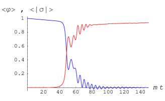
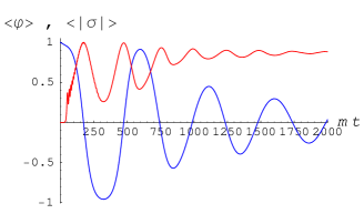
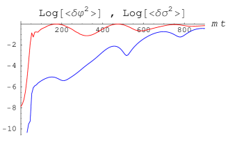
Figure 2: The left and middle panels show the evolution with time of the inflaton’s mean normalized to $\phi_{c}$ (blue), $\langle\phi/\phi_{c}\rangle$, and of the mean of the Higgs modulus normalized to its vev (red), $\langle|\sigma|/v\rangle$ (where $|\sigma|^{2}=\sigma_{1}^{2}+\sigma_{2}^{2}$), for $\lambda/g^{2}=0.5$ (left panel) and $\lambda/g^{2}=2000$ (middle panel). The other parameters are $V_{c}=10^{-3}$ and $\lambda=10^{-5}$ in both cases. The right panel shows the evolution with time of the variances $\mathrm{Log}[\langle\delta\phi^{2}/\phi_{c}^{2}\rangle]$ (blue) and $\mathrm{Log}[\langle\delta\sigma^{2}/v^{2}\rangle]$ (red) for the case $\lambda/g^{2}=2000\,$.

Fig. 2 shows the evolution with time of the averages $\langle\phi\rangle$ and $\langle|\sigma|\rangle$ (in the case of significant velocity at the preheating onset), for $g^{2}\sim\lambda$ (left panel) and $g^{2}<<\lambda$ (middle panel), and the same values of the other parameters. The right panel shows the evolution with time of the variances of the fields in the case $g^{2}<<\lambda$. One sees clearly the large inflaton oscillations around the true minimum, roughly from $\phi_{c}$ to $-\phi_{c}$ for the first oscillations in the case of the middle panel of Fig. 2. Note in particular that each time the inflaton approaches $\pm\phi_{c}$, the minimum in the $\sigma$-direction is at $\sigma=0$, so that $\sigma$ rolls back towards the origin where the symmetry is restored.

In both cases of Fig. 2, $\langle|\sigma|\rangle$ is first rapidly amplified up to a value a few times smaller than its VEV by the tachyonic effect as $\phi$ rolls slowly away from $\phi_{c}$ due to its initial velocity. The typical momentum amplified by this process is given by (8) and is independent of $g^{2}/\lambda$. After that stage, non-linearities become significant. Because of the amplification of $\sigma$, $\phi$ acquires an effective mass which makes it roll faster towards $\phi=0$. This happens much more slowly for $g^{2}<<\lambda$ since $m_{\phi}$ is much smaller in that case. As $\phi$ decreases, the tachyonic mass of $\sigma$ momentarily increases, which amplifies further $\sigma$ fluctuations until backreaction shuts off the tachyonic effect. For $g^{2}\mathrel{\hbox{\hbox to0.0pt{\hbox{\lower 4.0pt\hbox{$\sim$}}\hss}\hbox{$>$}}}\lambda$, the field distributions then rapidly settle around the true minimum, with dispersions $|\delta\sigma|\sim v$ and $|\delta\phi|\sim\phi_{c}$. On the other hand, for $g^{2}<<\lambda$, we still have $|\delta\phi|<<\phi_{c}$, see the right panel of Fig. 2.

We can further study this stage by noting that the trajectory of the field distributions in field space is quite accurately given for some time (up to $mt$ of order $600$ in the case $\lambda/g^{2}=2000$ of the middle panel of Fig. 2) by the ellipse

$$\lambda\,\sigma^{2}+g^{2}\,\phi^{2}=\lambda\,v^{2}\;,$$ (17)

which is essentially the condition $\partial V/\partial\sigma=0$. This is satisfied when $|\phi|<\phi_{c}$, see Fig. 1 for illustration. Along this trajectory, the potential reduces to

$$V=\frac{g^{2}}{2}\,v^{2}\,\phi^{2}-\frac{g^{4}}{4\,\lambda}\,\phi^{4}\ ,$$ (18)

and the dynamics corresponds to a single-field system with effective mass

$$\frac{m^{2}_{\phi}}{m^{2}}=\frac{g^{2}}{\lambda}\,\left(1-3\,\frac{\phi^{2}}{\phi_{c}^{2}}\right)\ ,$$ (19)

where $\langle\phi^{2}\rangle\,\simeq\,\langle\phi\rangle^{2}$ at that stage. We see that the mass squared becomes negative each time that $|\phi|>\phi_{c}/\sqrt{3}$. This leads to the tachyonic growth of modes with typical momenta

$$k_{*}\sim g\,v\,.$$ (20)

Note that this is much smaller than (8) for $g^{2}<<\lambda$. One can clearly see these successive tachyonic growths after the first, much more rapid amplification, in the right panel of Fig. 2. The successive tachyonic growths and the resulting bubble inhomogeneities will lead to succesive bursts of GW productions. We will confirm this effect numerically in Section VC.

In addition to these tachyonic growths, there are other non-adiabatic amplifications when $m_{\phi}(\phi)\approx 0$, which significantly affect the spectrum of $\phi$ fluctuations. This is very similar to the preheating process in models of new inflation Desroche:2005yt . Indeed, for the potential (18) the non-adiabaticity condition on the frequency, $|\dot{\omega}|\mathrel{\hbox{\hbox to0.0pt{\hbox{\lower 4.0pt\hbox{$\sim$}}\hss}\hbox{$>$}}}\omega^{2}$, reads $\left(k^{2}+m^{2}_{\phi}\right)^{3/2}\mathrel{\hbox{\hbox to0.0pt{\hbox{\lower 4.0pt\hbox{$\sim$}}\hss}\hbox{$<$}}}3\,|\phi|\,|\dot{\phi}|\,g^{4}/\lambda$. This is most easily satisfied around $\phi\approx\pm\phi_{c}/\sqrt{3}$, where $m_{\phi}\approx 0$. At that point, $|\dot{\phi}|$ may in principle depend on the initial inflaton velocity during the first oscillations, but for the last few non-adiabatic amplifications a good approximation is given by $|\dot{\phi}|\sim\sqrt{2\lambda}\,v^{2}/3$. This leads to the growth of modes with $k^{2}\mathrel{\hbox{\hbox to0.0pt{\hbox{\lower 4.0pt\hbox{$\sim$}}\hss}\hbox{$<$}}}g\,v$ around $\phi\approx\pm\phi_{c}/\sqrt{3}$. The typical momentum is lower by a factor of $2$ or so, $k_{*}\approx g\,v/2$.

Inserting this result into Eqs. (6), (7) gives

$$f_{*} \sim \frac{g}{\sqrt{\lambda}}\,\lambda^{1/4}\;3\times 10^{10}Hz\ ,$$ (21)

$$h^{2}\Omega^{*}_{gw} \sim 8\times 10^{-6}\,\frac{\lambda}{g^{2}}\,\left(\frac{v}{M_{\mathrm{Pl}}}\right)^{2}\,.$$ (22)

Note that this does not depend anymore on the initial velocity $V_{c}$. Compared to (9, 10), we see that usually the peak frequency decreases and the peak amplitude increases for $g^{2}<<\lambda\,$.

Since Eqs. (21), (20) do not depend on the initial tachyonic amplification, we expect them to hold also in the case of negligible initial velocity. Note that, in this case, it is more difficult than in (15) to lower $f_{*}$ with small coupling constants. Thus it is observationally more interesting to have $g^{2}\mathrel{\hbox{\hbox to0.0pt{\hbox{\lower 4.0pt\hbox{$\sim$}}\hss}\hbox{$>$}}}\lambda$ in the case of negligible initial velocity.

IV Calculation of Gravity Waves

In this Section we refine the basic method of GW calculations that we developed in DBFKU .

The energy density of gravity waves is constructed from the amplitude of the transverse-traceless part of the metric perturbation $h_{ij}$. The TT part can be extracted by applying a momentum-space projection operator $O_{ijlm}(k)$ (see e.g. DBFKU ), but this requires calculating the metric perturbations in momentum space. Alternatively, following juan2 , we can solve the position-space evolution equations for the whole $h_{ij}$ and then, when calculating gravity wave spectra, apply the projection operator to the end-point of the evolution results. Since the equations of motion and the projection operator are both linear they commute.

The equation of motion for the metric perturbations is

$$\bar{h}_{ij}^{\prime\prime}-\nabla^{2}\bar{h}_{ij}-{a^{\prime\prime}\over a}\bar{h}_{ij}=16\pi Ga^{3}\Pi_{ij}^{TT},$$ (23)

where we are using conformal time $d\tau=dt/a$ and metric perturbations $\bar{h}_{ij}=ah_{ij}$. We will use the non-TT source term

$$\Pi_{ij}={1\over a^{2}}\partial_{i}\phi\partial_{j}\phi\ ,$$ (24)

and compensate by applying the projection operator (in momentum space) to the resulting $\bar{h}_{ij}$. The other terms in the energy-momentum tensor vanish under the TT projection. The results of this calculation read as

$$\bar{h}_{ij}(\tau,\mathbf{k})=\frac{16\pi G}{k}\,\int_{\tau_{i}}^{\tau}d\tau^{\prime}\ \,{\cal G}\left[k\,(\tau,\tau^{\prime})\right]\,a(\tau^{\prime})\,T_{ij}^{\mathrm{TT}}(\tau^{\prime},\mathbf{k})\ ,$$ (25)

where ${\cal G}$ is the Green’s function of the operator $\partial^{2}_{t}+k^{2}-{a^{\prime\prime}\over a}$. In the typical case of power-law growth of the scale factor, $a(t)\sim t^{\alpha}$, the Green’s function is easily constructed from Bessel functions, and may have different behaviours for the sub- and super-horizon modes. During preheating, the equation of state $w$ usually jumps rapidly to a value close to $1/3$ eos . In a radiation-dominated universe we can put ${a^{\prime\prime}\over a}=0$. In this case the general solution (25) acquires a simple form

$$\bar{h}_{ij}(\tau,\mathbf{k})=\frac{16\pi G}{k}\,\int_{\tau_{i}}^{\tau}d\tau^{\prime}\ \,\sin\left[k\,(\tau-\tau^{\prime})\right]\,a(\tau^{\prime})\,T_{ij}^{\mathrm{TT}}(\tau^{\prime},\mathbf{k})\ ,$$ (26)

which can be matched to the source-free solution to give, at late times

$$\bar{h}_{ij}(\tau,\mathbf{k})=A_{ij}(\mathbf{k})\,\sin\left[k(\tau-\tau_{f}\ )\right]+B_{ij}(\mathbf{k})\,\cos\left[k(\tau-\tau_{f})\right]\;\;\;\;\mbox{ for }\;\ \;\;\tau\geq\tau_{f},$$ (27)

where

$$A_{ij}(\mathbf{k}) = \frac{16\pi G}{k}\,\int_{\tau_{i}}^{\tau_{f}}d\tau^{\prime}\,\cos\left[k\,(\tau_{f}-\tau^{\prime})\right]\,a(\tau^{\prime})\,T_{ij}^{\mathrm{TT}}(\tau^{\prime},\mathbf{k})$$

$$B_{ij}(\mathbf{k}) = \frac{16\pi G}{k}\,\int_{\tau_{i}}^{\tau_{f}}d\tau^{\prime}\,\sin\left[k\,(\tau_{f}-\tau^{\prime})\right]\,a(\tau^{\prime})\,T_{ij}^{\mathrm{TT}}(\tau^{\prime},\mathbf{k})\ .$$ (28)

Once we have Fourier transformed the metric perturbations and projected out the TT part the gravity wave energy density can be calculated as

$$\rho_{gw}={1\over 32\pi Ga^{4}}{1\over V}\int d^{3}k\bar{h}_{ij}^{\prime}(\vec{k})\bar{h}_{ij}^{\prime*}(\vec{k})\ ,$$ (29)

where summation over $i$ and $j$ is understood. However, this formula will include small time oscillations of the modes, given by the sine and cosine terms in Eq. (27) above. In our Fourier space calculations we eliminated these oscillations by averaging over a full period, thus replacing $\bar{h}_{ij}^{\prime}(k)\bar{h}_{ij}^{\prime*}(k)$ with $(k^{2}/2)\left(|A_{ij}|^{2}+|B_{ij}|^{2}\right)$. We can accomplish the same thing in this calculation by noting that at time $\tau=\tau_{f}$ we have $B_{ij}=\bar{h}_{ij}$, $A_{ij}=\bar{h}_{ij}^{\prime}/k$, so we can calculate the energy density averaged over a full oscillation as

$$\rho_{gw}={1\over 32\pi Ga^{4}}{1\over V}\int d^{3}k{k^{2}\over 2}\left(|\bar{h}_{ij}|^{2}+{1\over k^{2}}|\bar{h}_{ij}^{\prime}|^{2}\right)={1\over 64\pi Ga^{4}}{1\over V}\int d^{3}k\left(k^{2}|\bar{h}_{ij}|^{2}+|\bar{h}_{ij}^{\prime}|^{2}\right)\ .$$ (30)

We use the notation $|X_{ij}|^{2}=\sum_{i,j}X_{ij}X_{ij}^{*}$.

By assuming isotropy we can write

$${1\over 16Ga^{4}}{1\over V}\int dkk^{2}\left(k^{2}|\bar{h}_{ij}|^{2}+|\bar{h}_{ij}^{\prime}|^{2}\right)\ .$$ (31)

The gravity wave spectrum can then be calculated as

$$S_{k}\equiv a^{4}k{d\rho_{gw}\over dk}={k^{3}\over 16GV}\left(k^{2}|\bar{h}_{ij}|^{2}+|\bar{h}_{ij}^{\prime}|^{2}\right)\ .$$ (32)

We make a couple of remarks about the formulas (30)-(32). As we demonstrated in DBFKU , in the limit of $\tau_{f}\to\infty$ and $a(t)\to const$, we recover Weinberg’s formula for the emission of GW from isolated sources in flat space-time. Next, the forms (30)-(32) admit a natural interpretation in terms of a number density of emitted gravitons. Indeed, from the oscillating amplitudes $\bar{h}_{ij}(\vec{k},\tau)$ one can construct the adiabatic invariant

$$n_{k}=\frac{1}{2k}\left(k^{2}|\bar{h}_{ij}|^{2}+|\bar{h}_{ij}^{\prime}|^{2}\right)\ ,$$ (33)

which corresponds to the number of gravitons per mode $\vec{k}$. Then, Eq. (30) can be re-interpreted in terms of the energy density carried out by the gravitons

$$\rho_{gw}={1\over 32\pi Ga^{4}}{1\over V}\int d^{3}k\,k\,n_{k}\ .$$ (34)

Correspondingly, $S_{k}={k^{4}n_{k}\over 8GV}$.

From Eq. (32), the derivation of today’s spectrum occurs as it did with our Fourier space calculation, adapted for the hybrid inflation case as discussed below. In the chaotic inflation case we evolved the spectrum to today by defining a time $t_{j}$ at the end of the simulation after which we took the equation of state to be $w=1/3$. In the case of hybrid inflation, we are not considering expansion during preheating and we assume that the equation of state approaches $w=1/3$ within a few Hubble times afterwards, so we effectively take $t_{j}$ to be the end of inflation, and simply evolve to today’s variables with

$$f={k\over\rho^{1/4}}(4\times 10^{10}Hz)\ ,$$ (35)

$$\Omega_{gw}h^{2}=(9.3\times 10^{-6}){S_{k}(\tau_{f})\over\rho}\ ,$$ (36)

where we take $\rho=(1/4)\lambda v^{4}$.

In the next Section we will describe results of numerical calculations of GW from lattice simulations of tachyonic preheating. However, the infra-red (IR) tail of the spectrum, which is often interesting for observations, is not captured by the finite-size simulations. Eq. (26) is useful for deriving the IR asymptotics of the gravity wave spectrum. For momenta small compared to the peak of the scalar field spectra, $k<<k_{*}$, the convolution of the scalar field spatial derivatives is independent of $\mathbf{k}$, $T_{ij}^{\mathrm{TT}}(\tau^{\prime},\mathbf{k})\simeq T_{ij}^{\mathrm{TT}}(\tau^{\prime},0)$. This corresponds to the quadrupole approximation. We can then distinguish two different regimes, depending on the time variation of the Green’s function $\sin\left[k\,(\tau-\tau^{\prime})\right]$ and the source $T_{ij}^{\mathrm{TT}}(\tau^{\prime},0)$. For sufficiently small $k$, the Green’s function varies more slowly than the source and may be taken out of the integral in (26). This gives $\Omega_{gw}\propto f^{3}$ for the IR tail of the GW spectrum (36), (32). On the other hand, there can be an intermediate frequency range between the IR tail and the peak where $\sin\left[k\,(\tau-\tau^{\prime})\right]$ varies more rapidly than $T_{ij}^{\mathrm{TT}}(\tau^{\prime},0)$. The time integral in (26) then gives an extra $1/k$ factor, leading to $\Omega_{gw}\propto f$ for some frequency range below the peak. In the transitional region we expect a power-law slope, $\Omega_{gw}\propto f^{\gamma}$ with $\gamma$ varying between 1 and 3. For the model of parametric resonance that we considered in DBFKU , we observed the $\Omega_{gw}\propto f$ behaviour. For tachyonic preheating, however, the source varies typically with a characteristic time given by $1/k_{*}$, i.e. more rapidly than the Green’s function for any $k<k_{*}$. Therefore, we expect the IR tail $\Omega_{gw}\propto f^{3}$ to be valid quickly below the peak. For the IR part of the spectrum just below the peak that we can probe in our simulations, we found $\gamma\sim 2-2.5$. The exact value was different for the three cases of significant initial velocity, negligible initial velocity and $g^{2}<<\lambda$, but it was the same in all our numerical results for a given case.

V Numerical Results and Parameter Dependence

In this section we report the results of numerical calculations of GW radiation from tachyonic preheating after hybrid inflation. Some technical details of the numerical simulations are described in the Appendices. In particular, we study how the gravity wave characteristics depend on the parameters of the hybrid model. This will allow us to directly check our analytical estimates and find fits for the peak frequency and amplitude. The analytical estimates of Section III were based on the picture of a sudden growth of the density “bubbles” associated with the high peaks of the random gaussian fields of initial quantum fluctuations. Therefore we begin this Section with an illustration of the growth of these bubbles, shown in Fig. 3. The four panels show the field amplitude (left of each panel) and GW energy density (right of each panel) at four moments of time on a two-dimensional slice through the three-dimensional lattice. The initial bump of the field produces an exponentially growing bubble, and we can clearly see a burst of GW radiating from this growing bubble. The background stochastic GW radiation is the superposition of such concentric bursts.

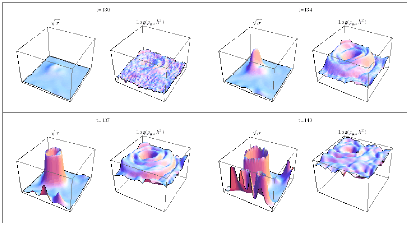
Figure 3: Field amplitude and gravity wave density as a function of space on a two dimensional slice through the lattice. The slice is chosen at the height where the first Higgs bubble appeared. The simulation is of the model (1) with $\lambda=10^{-5}$, $\lambda/g^{2}=0.5$, $v=10^{-3}$, and $V_{c}=0$.

The configuration space picture of Fig. 3 is complemented by the momentum space spectra of gravity waves.

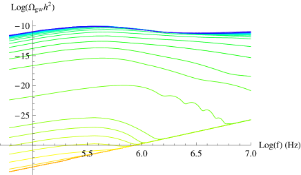
Figure 4: Gravity wave spectra for the model (1) with $\lambda=10^{-14}$, $\lambda/g^{2}=0.5$, $v=10^{-3}$, and $V_{c}=10^{-5}$. Lower (red) curves correspond to earlier moments of the simulation and higher (bluer) curves are from later moments of the simulation. All results are scaled to the present-day spectrum.

Fig. 4 shows the gravity wave spectra from the lattice simulation with one representative set of parameters corresponding to the case $\lambda/g^{2}=1/2$ and the onset of preheating dominated by classical rolling. All spectra shown in this paper are scaled to present-day units. The different curves show cumulative results for different moments of times during the simulation. For some time after inflation no gravity waves are produced, then there is a burst of growth during preheating, and then the spectrum saturates at a stationary level. A clear peak frequency is established early in the growth and remains roughly constant as the amplitude grows.

As noted above, the model (1) involves essentially four parameters related to preheating: the coupling constants $\lambda$ and $g$, the symmetry breaking VEV $v$, and the unitless field velocity at the critical point, $V_{c}$.

First, we discuss how GW spectra calculated from lattice simulations depend on the parameters in the case where $\lambda=2g^{2}$. From the point of view of numerical simulations this is the simplest case because there is no gap between different mass scales. Later we will study how the results depend on the ratio $g^{2}/\lambda$.

As noted in Section II, the dependence of the spectra on $v$ can be calculated analytically in the absence of expansion. Specifically, changing $v$ does not shift the frequencies at all and changes the density in gravity waves today proportionally to $v^{2}$. This result should hold as long as $v$ is small enough to maintain the waterfall condition.

As we anticipated in Section III, variation with $V_{c}$, the inflaton velocity at the bifurcation point, results in significant variations of the GW spactra. For the case with significant initial velocity Eqs. (9), (10) accurately predict the peak frequency and amplitude to within an order of magnitude for all of the parameters we have tested, which includes initial velocities ranging from $V_{c}=10^{-5}$ to $10^{-2}$ for $\lambda=10^{-14}$ and $10^{-5}$.

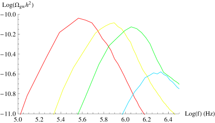
Figure 5: Dependence of GW final spectra on $V_{c}$. The curves from left to right correspond to $V_{c}=10^{-5}$, $V_{c}=10^{-4}$, $V_{c}=10^{-3}$, and $V_{c}=10^{-2}$. Here $\lambda=10^{-14}$.

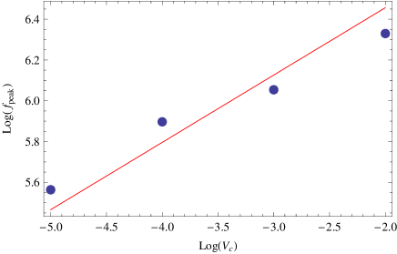
Figure 6: The peak frequency for the gravity wave spectrum as a function of initial velocity for $\lambda=10^{-14}$. The line shows the slope of the prediction (9) with the overall height adjusted to fit the data.

Fig. 6 shows the final gravity wave spectra for a range of initial velocities for $\lambda=10^{-14}$. Increases in $V_{c}$ lead to increases in peak frequency and decreases in peak amplitude, but the shape of the spectra are quite similar. Fig. 6 shows the numerical peak frequencies for the cases from Fig. 6. Eq. (9) predicts that $f_{peak}\propto V_{c}^{1/3}$ so the figure shows a best-fit line with slope $1/3$, illustrating that the dependence matches the prediction. The actual values of the peak frequencies are all within a factor of $3$ of the Eq. (9), which is in any case only an order of magnitude estimate.

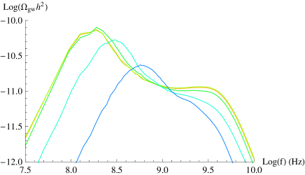
Figure 7: Final gravity wave spectra after preheating for $\lambda=10^{-5}$. The plots from left to right show $V_{c}=:0,10^{-6},10^{-5},V_{c}=10^{-4},10^{-3},10^{-2}$. The plots for $V_{c}=0,10^{-6}$, and $10^{-5}$ lie almost perfectly on top of each other.

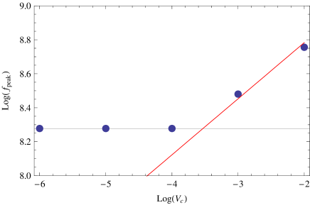
Figure 8: The peak frequency for the gravity wave spectrum as a function of initial velocity for $\lambda=10^{-5}$. The line shows the slope of the prediction (9) with the overall height adjusted to fit the last two points. The horizontal line is the peak frequency for $V_{c}=0$. For $V_{c}\mathrel{\hbox{\hbox to0.0pt{\hbox{\lower 4.0pt\hbox{$\sim$}}\hss}\hbox{$<$}}}10^{-4}$ the peak remains constant at the $V_{c}=0$ value.

Eq. (9) is not expected to be accurate in the limit of very low initial velocities, as discussed in sub-section III.2. For example, Figs. 8-8 show the spectra and peak frequencies for $\lambda=10^{-5}$. For this larger value of $\lambda$ the formula (9) fails for $V_{c}\mathrel{\hbox{\hbox to0.0pt{\hbox{\lower 4.0pt\hbox{$\sim$}}\hss}\hbox{$<$}}}10^{-4}$. Figure 8 shows that the spectra for $V_{c}=10^{-5}$ and $V_{c}=10^{-6}$ are nearly identical to the $V_{c}=0$ spectrum, so below $V_{c}\mathrel{\hbox{\hbox to0.0pt{\hbox{\lower 4.0pt\hbox{$\sim$}}\hss}\hbox{$<$}}}10^{-4}$ there is no $V_{c}$ dependence. The fit shown in this figure once again has the slope predicted by Eq. (9) and a height adjusted to fit the data, but in this case the fit is to the last two points only. The actual values for peak frequency for these last two points match Eq. (9) to within a factor of $2$.

For lower $\lambda$, such as the results shown above, the initial velocity for which quantum diffusion dominates is much lower and thus the results in Fig. 6 show the $V_{c}^{1/3}$ dependence discussed above.

For $g^{2}=2\lambda$, our estimate (14) indicates that the velocity $V_{c}$ could be considered negligible below the cutoff $V_{c}\approx C^{3}\,\lambda^{3/2}$. From the data above we conclude that for $\lambda=10^{-5}$ this cutoff occurs between $V_{c}=10^{-5}$ and $V_{c}=10^{-4}$, which means $C\approx 10$. It is hard to estimate, however, if this value is independent of $\lambda$. For lower values of $\lambda$ we were unable to simulate slow enough initial velocities to see the crossover between these two regimes. We can thus only conjecture that this value $C\approx 10$ will be roughly constant for different values of $\lambda$. This conjecture must be true if our predicted dependence $f_{peak}\propto\lambda^{3/4}$ is correct for the case of negligible initial velocity.

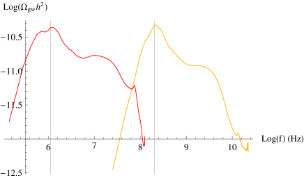
Figure 9: Gravity wave spectra for $\lambda=10^{-14}$ (left) and $\lambda=10^{-5}$ (right), each with $V_{c}=10^{-3}$. The vertical line through the $\lambda=10^{-5}$ peak marks the maximum of that peak. The vertical line through the $\lambda=10^{-14}$ peak is a prediction based on extrapolating the $\lambda=10^{-5}$ peak frequency assuming $f_{peak}\propto\lambda^{1/4}$.

Next, we investigate an impact of variation with $\lambda$ on the GW production. For the case with significant initial velocity $V_{c}$ the equations above predict that changing $\lambda$ should not change the amplitude but should simply shift the frequency as $f_{peak}\propto\lambda^{1/4}$. Fig. 9 clearly shows this to be the case.

As discussed above, we can not numerically test the dependence of the spectrum on $\lambda$ for the case of negligible initial velocity, but we believe our predictions should be accurate for this case because at low initial velocity the bubble description of preheating is accurate.

We now discuss how our numerical results for the gravity wave spectrum depend on the ratio $g^{2}/\lambda\,$. For a given inflationary potential $V_{\mathrm{inf}}(\phi)$, changing $g^{2}/\lambda$ changes the critical point $\phi_{c}$ and the unitless velocity $V_{c}$ at that point, see (3). However, in order to isolate the $g^{2}/\lambda$ dependence, we will keep $V_{c}$ constant in this section. We first consider the case of non-negligible initial velocity.

In this case, gravity wave spectra for different values of $g^{2}/\lambda$ are shown in Fig. 10, for $V_{c}=10^{-3}$. For $g^{2}\mathrel{\hbox{\hbox to0.0pt{\hbox{\lower 4.0pt\hbox{$\sim$}}\hss}\hbox{$>$}}}\lambda$, the peak frequency and amplitude are roughly independent of $g^{2}/\lambda$, in agreement with our original prediction, Eqs. (9), (10). (When $g^{2}$ increases, rescattering effects become more important and the UV part of the GW spectrum has higher amplitude). On the other hand, for $g^{2}<<\lambda$, it is clear from Fig. 10 that decreasing $g^{2}/\lambda$ decreases the peak frequency and increases the peak amplitude, in aggreement with Eqs. (21), (22). Note also that, for a given value of $g^{2}/\lambda<<1$, the dependence on $\lambda$ is very well given by $f_{*}\propto\lambda^{1/4}$ and $h^{2}\,\Omega^{*}_{\mathrm{gw}}$ independent of $\lambda$, again in agreement with Eqs. (21), (22). Note that Fig. 10 shows the gravity wave spectrum for $v=10^{-3}\,M_{\mathrm{Pl}}$. For $g^{2}<<\lambda\,$, a lower value of $v$ may be necessary to consistently neglect the expansion of the universe, as discussed below. Lowering $v$ leaves the shape of the spectra unchanged but reduces their amplitude proportionally to $v^{2}$.

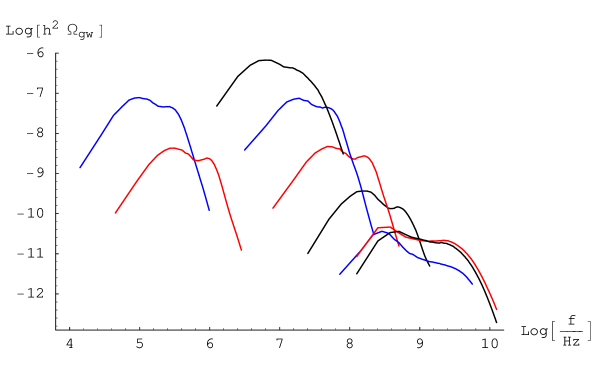
Figure 10: Numerical results for the gravity wave spectra for several values of $\lambda/g^{2}$, for $\lambda=10^{-14}$ (left) and $\lambda=10^{-5}$ (right), each with $V_{c}=10^{-3}$. The spectra for $\lambda=10^{-5}$ (right) are, from top to bottom, for $\lambda/g^{2}$ $=$ $20000$ (black), $5000$ (blue), $500$ (red), $50$ (black), $0.5$ (blue), $0.005$ (red) and $0.0005$ (black). The spectra for $\lambda=10^{-14}$ (left) are for $\lambda/g^{2}$ $=$ $5000$ (top, blue) and $500$ (bottom, red). To ease the comparison, all the spectra are shown for $v=10^{-3}\,M_{\mathrm{Pl}}$, although for $g^{2}<<\lambda$ a lower value of $v$ may be necessary to consistently neglect expansion of the universe (see the main text for details). This lowers the spectra as $h^{2}\,\Omega_{\mathrm{gw}}\propto v^{2}$. In other words, the $y$-axis of the plot is really the log of $h^{2}\,\Omega_{\mathrm{gw}}/(10^{3}\,v/M_{\mathrm{Pl}})^{2}\,$.

Decreasing $g^{2}/\lambda$ results in qualitatively different GW production. Fig. 11 shows the accumulation with time of the total energy density in gravity waves for two cases, the left panel for $g^{2}\sim\lambda$ and the right panel for $g^{2}<<\lambda$. In the first case we see a single burst of GW production from tachyonic preheating. In the second case, we clearly see successive bursts of gravity wave production, due to the successive tachyonic and non-adiabatic amplifications discussed in subsection III.3, and the subsequent bubble collisions. Because the characteristic time scale in this case is given by $m\,\sqrt{\lambda}/g\,$, for $g^{2}<<\lambda$ preheating and gravity wave production take more time than for $g^{2}\sim\lambda$. As a result, the upper bound on $v$ necessary for the expansion of the universe to be negligible is lower than for $g^{2}\mathrel{\hbox{\hbox to0.0pt{\hbox{\lower 4.0pt\hbox{$\sim$}}\hss}\hbox{$>$}}}\lambda$. This decreases the maximum GW amplitude as $h^{2}\,\Omega_{\mathrm{gw}}\propto v^{2}$. If the peak of the gravity wave spectrum is reached after a proper time $\tau\,$, we require it to be much smaller than the Hubble time

$$\frac{\tau}{H^{-1}}\,\approx\,m\,\tau\;\frac{v}{M_{\mathrm{Pl}}}<<1\,.$$ (37)

Figure 11: Evolution with time of the total energy density in gravity waves, $\rho_{\mathrm{gw}}/(10^{3}\,v/M_{\mathrm{Pl}})^{2}\,$, for $\lambda/g^{2}=0.5$ (left) and $\lambda/g^{2}=2000$. The parameters are the same as in Fig. 2.

In fact, for all the cases with $g^{2}<<\lambda$ that we considered, the peak amplitude of the GW spectrum continued to slightly but constantly increase with time after the last burst of GW production (i.e. after $m\,t\sim 1000$ for the right panel of Fig. 11), and the peak frequency tended to move further towards the infrared. However, if we consider very late times expansion will become significant, thus invalidating the results of our simulations. For low values of $v$ this growth could continue longer without being diluted by expansion, but the overall amplitude would be lower. For each set of parameters $\lambda$, $g$, and $V_{c}$ there is thus an optimal value of $v$ that will produce the greatest amplitude of gravity waves before expansion becomes significant. For each set of parameters $\lambda$, $g$, and $V_{c}$ we define $v_{opt}$ to be this optimal value and we define the time $\tau$ as the time at which expansion would become significant for $v=v_{opt}$. The spectra shown in Fig. 10 were obtained at that time.

Figure 12: Peak frequency $f_{*}$ (left), peak amplitude $h^{2}\,\Omega^{*}_{\mathrm{gw}}$ (middle) and time $m\,\tau$ defined in the main text (right), for $V_{c}=10^{-3}$, $\lambda=10^{-5}$, $v=10^{-3}$, and several values of $g^{2}/\lambda<<1$. The lines shown are the best linear fits for all the points except the one with $\lambda/g^{2}=20000$ (extreme right): $f_{*}\propto(\lambda/g^{2})^{-1/2}$, $h^{2}\Omega^{*}_{\mathrm{gw}}\propto(\lambda/g^{2})^{1.16}$ and $m\tau\propto(\lambda/g^{2})^{0.53}\,$.

Fig. 12 shows in the left panel: the peak frequency, in the middle: the peak amplitude and in the right: the time $m\,\tau$ defined above, for $V_{c}=10^{-3}$, $\lambda=10^{-5}$ and several values of $g^{2}/\lambda<<1\,$. We see that the prediction (21), $f_{*}\propto g$, is very well satisfied. The peak amplitude grows slightly more rapidly than (22) when $g^{2}/\lambda$ decreases, $h^{2}\,\Omega^{*}_{\mathrm{gw}}\propto(\lambda/g^{2})^{1.16}\,$. Finally, $m\,\tau$ grows slightly more rapidly than $\sqrt{\lambda}/g\,$, $m\tau\propto(\lambda/g^{2})^{0.53}\,$. In these fits, we disregarded the point at the extreme right ($\lambda/g^{2}=20000$), which is slightly displaced compared to the others. In fact, for $\lambda/g^{2}\mathrel{\hbox{\hbox to0.0pt{\hbox{\lower 4.0pt\hbox{$\sim$}}\hss}\hbox{$>$}}}10^{4}\,$, and for the initial velocity $V_{c}=10^{-3}$ considered here, the inflaton reached $|\phi|>\phi_{c}$ and spent most of the time in these regions. Indeed, in these regions, the minimum in the $\sigma$-direction is at $\sigma=0$ and the effective mass for $\phi$ is very low, $m^{2}_{\phi}=g^{2}\,\langle\sigma^{2}\rangle$. Apparently, this slightly increases the peak amplitude and decreases the peak frequency. However, it may not be a good approximation to neglect $V_{inf}(\phi)$ in the region where $|\phi|>\phi_{c}\,$. Also, we decreased $g^{2}/\lambda$ while keeping $V_{c}$ fixed. However, for a given physical initial velocity $\dot{\phi}_{c}\,$, decreasing $g^{2}/\lambda$ decreases the unitless velocity $V_{c}\,$, see (3). For sufficiently small $V_{c}\,$, the inflaton will not reach values $|\phi|>\phi_{c}\,$. We will thus neglect this effect below, although it may be useful to further decrease the peak frequency.

We then obtain the following fits for the peak frequency and amplitude of the GW spectrum for the case $g^{2}/\lambda<<1$

$$f_{*}\simeq\frac{g}{\sqrt{\lambda}}\,\lambda^{1/4}\,10^{10.25}\;\mathrm{Hz}$$ (38)

$$h^{2}\,\Omega^{*}_{\mathrm{gw}}\simeq 10^{-5.5}\;\left(\frac{\lambda}{g^{2}}\right)^{1.16}\;\left(\frac{v}{M_{\mathrm{Pl}}}\right)^{2}\,.$$ (39)

From the fit of $m\,\tau$, the constraint (37) for the expansion of the universe to be negligible becomes

$$\frac{v}{M_{\mathrm{Pl}}}<<10^{-1.3}\;\left(\frac{\lambda}{g^{2}}\right)^{-0.53}\,.$$ (40)

Note that this condition always implies $\phi_{c}<<M_{\mathrm{Pl}}\,$. Together with (39), it also implies $h^{2}\,\Omega^{*}_{\mathrm{gw}}<<10^{-8.1}\,(\lambda/g^{2})^{0.1}\,$.

For instance, for $\lambda\sim 0.1$, $f_{*}\mathrel{\hbox{\hbox to0.0pt{\hbox{\lower 4.0pt\hbox{$\sim$}}\hss}\hbox{$<$}}}10^{3}\,\mathrm{Hz}$ for $g^{2}\mathrel{\hbox{\hbox to0.0pt{\hbox{\lower 4.0pt\hbox{$\sim$}}\hss}\hbox{$<$}}}10^{-15}\,$, and the amplitude (39) may be relevant for Advanced LIGO while satisfying the constraint (40).

We expect similar results as above in the case of negligible velocity $V_{c}$. In this case, where quantum diffusion dominates, observationally more interesting results can be obtained without the requiremenet $g^{2}<<\lambda$.

VI Discussion and Perspectives

In this paper, we studied the stochastic background of gravitational waves produced from tachonic preheating after hybrid inflation in the very early universe. The present-day frequencies and amplitudes of these gravity waves may cover a wide range of values, depending on the main phenomenological parameters introduced in Section II: the VeV $v$ and self-coupling $\lambda$ of the symmetry breaking fields, their coupling to the inflaton $g^{2}$ and the (unitless) initial velocity of the inflaton at the critical point $V_{c}$. We developed analytical and numerical tools to calculate the resulting GW spectra and to study in detail how they depend on these parameters. We identified three dynamical regimes leading to qualitatively different results for the GW spectra produced from tachyonic preheating: (i) the case with $g^{2}\mathrel{\hbox{\hbox to0.0pt{\hbox{\lower 4.0pt\hbox{$\sim$}}\hss}\hbox{$>$}}}\lambda$ and the onset of preheating driven by the classical rolling of the inflaton, (ii) the case with $g^{2}\mathrel{\hbox{\hbox to0.0pt{\hbox{\lower 4.0pt\hbox{$\sim$}}\hss}\hbox{$>$}}}\lambda$ and quantum diffusion at the onset of preheating (corresponding to a negligible initial velocity of the inflaton at the bifurcation point) and (iii) the case with $g^{2}<<\lambda$ where GW are produced in successive bursts. Only the first case was considered in previous works about GW from tachyonic preheating juan1 ; juan2 , where the resulting GW spectrum was computed in the specific range $g^{2}\sim\lambda\sim V_{c}\sim\mathcal{O}(1)$.

Based on our results, we can determine the range of parameters of hybrid inflation models for which preheating may lead to a GW signal that is potentially observable. Let us first discuss the frequencies and amplitudes of stochastic GW backgrounds that are relevant for GW astronomy.

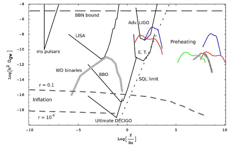
Figure 13: Expected sensitivities of interferometric experiments (adapted from buonanno ) compared to gravity wave spectra from tachyonic preheating in the cases of significant intial velocity with $g^{2}\mathrel{\hbox{\hbox to0.0pt{\hbox{\lower 4.0pt\hbox{$\sim$}}\hss}\hbox{$>$}}}\lambda$ (green), negligible initial velocity with $g^{2}\mathrel{\hbox{\hbox to0.0pt{\hbox{\lower 4.0pt\hbox{$\sim$}}\hss}\hbox{$>$}}}\lambda$ (red), and $g^{2}<<\lambda$ (blue). Also shown are the BBN and ms pulsar bounds, the stochastic background from extragalactic White Dwarfs binaries (taken from phinney ), the inflationary background for two values of the tensor to scalar ratio, and the spectrum from preheating in a $\lambda\,\phi^{4}$ model of chaotic inflation (double spectra in grey at the right, calculated with our previous code DBFKU ). The GW spectra from tachyonic preheating, for the peak from left to right, correspond to the following values of the parameters: (1) $\lambda=2g^{2}=10^{-14}$, $v=3\,10^{-7}\,M_{\mathrm{Pl}}$ and negligible initial velocity ; (2) $\lambda=0.1$, $g^{2}=10^{-16}$ and $v=3\,10^{-10}\,M_{\mathrm{Pl}}$ (independent of $V_{c}$) ; (3) $\lambda=2g^{2}=10^{-14}$, $v=10^{-3}\,M_{\mathrm{Pl}}$ and $V_{c}=10^{-3}$ ; (4) $\lambda=0.1$, $g^{2}=10^{-4}$ and $v=6\,10^{-4}\,M_{\mathrm{Pl}}$ (independent of $V_{c}$) ; (5) $\lambda=2g^{2}=10^{-5}$, $v=10^{-3}\,M_{\mathrm{Pl}}$ and negligible initial velocity.

We consider the present-day frequencies $f$ and the spectrum of energy density per logarithmic frequency interval $h^{2}\,\Omega_{\mathrm{gw}}(f)$. Fig. 13 shows the sketch of expected sensitivities of planned and future interferometric experiments: Advanced LIGO, LISA, the Einstein Telescope, Big Bang Observer and DECIGO (see buonanno for the relevant references). Note also the recent atomic interferometric sensor proposal of agis , which may be sensitive to GW backgrounds with frequencies in the range $1-10$ Hz and in the LISA range. We also show the BBN and ms pulsar bounds, and predictions for the stochastic GW background generated from inflation, for different values of the parameter $r$ (the ratio of the tensor and scalar amplitudes of the inflationary cosmological perturbations). Cosmological GW signals will be obscured by several expected astrophysical foregrounds, notably from White Dwarf binaries phinney , see Fig. 13.

There are also several bar and spherical resonant detectors (see e.g. minigrail ) operating in the kHz range. Other experiments have been proposed at higher frequencies, up to $100$ MHz Nishizawa:2007tn . However, the sensitivity to $h^{2}\,\Omega_{\mathrm{gw}}$ drops dramatically when the frequency increases. Indeed, we also have to take into account the current “Standard Quantum Limit”

$$h^{2}\,\Omega_{\mathrm{gw}}\sim\frac{10^{-17}}{x^{2}}\,\left(\frac{f}{Hz}\right)^{3}\ ,$$ (41)

shown in Fig. 13. The region on the right of this line is not observable with interferometric experiments due to the shot noise fluctuations of photons. Here $x$ is the squeezing parameter, which experimentalists are trying to push from one to a few.

Exemples of GW spectra from tachonic preheating calculated in this paper are shown in Fig. 13. We also show in this figure a GW spectrum from preheating after chaotic inflation calculated in DBFKU (the double-spectrum in grey), which is located in the high-frequency side and is not observable. GW from tachyonic preheating may cover a much wider range of frequencies, spreading from the highest frequencies shown in the figure to the region in between the SQL limit and the WD binaries, which is in principle observable . In each case shown in the figure, a lower Higgs VeV would lead to lower amplitudes and smaller coupling constants would lead to smaller frequencies.

Our analytical and numerical results for the peak frequency $f_{*}$ and the peak amplitude $h^{2}\,\Omega_{\mathrm{gw}}^{*}$ of the GW spectra are well described by Eqs. (9)-(10) in the case with $g^{2}\mathrel{\hbox{\hbox to0.0pt{\hbox{\lower 4.0pt\hbox{$\sim$}}\hss}\hbox{$>$}}}\lambda$ and the onset of preheating driven by the classical rolling of the inflaton, Eqs. (15)-(16) in the case with $g^{2}\mathrel{\hbox{\hbox to0.0pt{\hbox{\lower 4.0pt\hbox{$\sim$}}\hss}\hbox{$>$}}}\lambda$ and quantum diffusion at the onset of preheating (negligible initial velocity of the inflaton at the critical point) and Eqs. (38)-(39) in the case with $g^{2}<<\lambda$. The peak frequency depends essentially on the coupling constants and is independent of the Higgs VeV $v$. As a result, $\lambda\sim g^{2}\sim\mathcal{O}(1)$ leads to GW at very high frequencies, independent of the energy scale during inflation, and the only way to lower the frequency is to lower the coupling constants. On the other hand, $h^{2}\,\Omega_{\mathrm{gw}}^{*}\propto v^{2}$, so that at any frequency the amplitude can be relatively high for sufficiently high $v$, roughly up to the maximal bound  $h^{2}\Omega_{\mathrm{gw}}^{*}<10^{-6}\,$. Such a high energy density in GW implies in particular that these GW may already be observable by Advanced LIGO, but this generally requires very small coupling constant(s), see Fig. 13. For illustration, we show in Fig. 14, for each of the three cases discussed above, the range of parameters of the hybrid inflation models such that the peak frequency of the GW produced from preheating satisfy $f_{*}<10^{3}$ Hz. This is basically the condition for these gravity waves to be observable if $v$ is set to the maximum possible value consistent with the waterfall condition. In the first case of Fig. 14, corresponding to $g^{2}\mathrel{\hbox{\hbox to0.0pt{\hbox{\lower 4.0pt\hbox{$\sim$}}\hss}\hbox{$>$}}}\lambda$ and significant initial velocity, the coupling of interest $\lambda$ typically has to be extremely small, down to $\lambda<10^{-30}$ for $V_{c}\sim 1$. In the second case, with negligible initial velocity, we may have $g^{2}\sim\lambda\sim 10^{-11}$. In the third case ($g^{2}<<\lambda$), the most interesting regime corresponds to $\lambda\sim 1$, but this still requires $g^{2}<10^{-14}$.

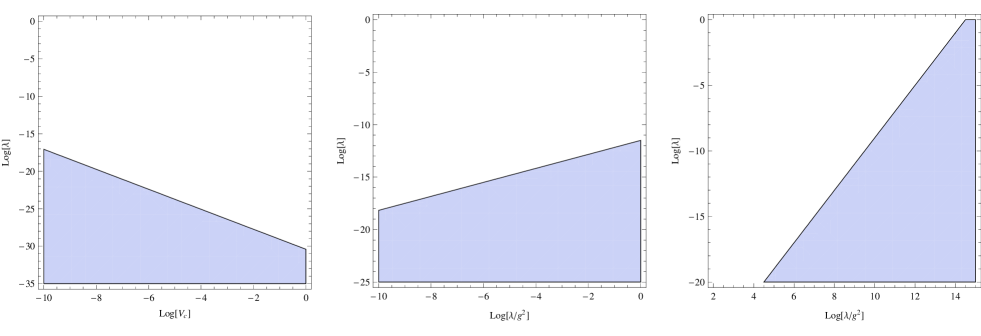
Figure 14: The regions of parameter space for which the peak of the gravity wave signal satisfies $f_{*}<10^{3}$ Hz. The panels show: Left - significant initial velocity and $g^{2}\mathrel{\hbox{\hbox to0.0pt{\hbox{\lower 4.0pt\hbox{$\sim$}}\hss}\hbox{$>$}}}\lambda$. Middle - negligible initial velocity and $g^{2}\mathrel{\hbox{\hbox to0.0pt{\hbox{\lower 4.0pt\hbox{$\sim$}}\hss}\hbox{$>$}}}\lambda$. Right - $g^{2}\ll\lambda$.

Above we focused on the peak frequency $f_{*}$ of the GW spectra. At lower frequencies, the spectra have a power-law tail, $\Omega_{\mathrm{gw}}\propto f^{\alpha}$. For tachyonic preheating, we found in this paper an intermediate regime with a relatively steep slope, $\alpha=2-2.5$, before the IR tail with $\alpha=3$ corresponding to the modes produced outside the Hubble radius. The infra-red part of the spectrum does not significantly improve the constraints on the parameters shown in Fig. 14. As outlined above, the range of parameters leading to the maximum amplitude in GW correspond to $k_{*}$ slightly below $H$. In this case, the spectra decrease as $\Omega_{\mathrm{gw}}\propto f^{3}$ for frequencies just below the peak. In particular, since this is the same dependence as the SQL limit (41), if the peak of the GW spectrum is located at the right of this line, the same is true for the IR tail.

In sum, our sober conclusion is that GW from tachyonic preheating after hybrid inflation can fall in the observable range of the $h^{2}\Omega_{\mathrm{gw}}--f$ plane that is currently conceivable only for uncomfortably small values of the coupling constants of the model.

We should note, however, that particle physics models of hybrid inflation with such small coupling constants have been considered. First, if the field $\sigma$ in the model (1) corresponds to a flat direction, we may expect its negative mass squared at the origin to be of the order $\lambda v^{2}\sim\mathrm{TeV}^{2}$, and the true minimum of the potential to be located at a VeV at a much higher scale, as high as $v\sim M_{\mathrm{Pl}}$. This gives a coupling constant as low as $\lambda\sim 10^{-30}$. Hybrid inflation models along this line have been proposed in randall ; stewart . Another model which, for the same reason, naturally involves very small coupling constants is thermal inflation thermal . Preheating mechanisms in this model have not been studied in detail yet, but tachyonic amplifications may lead to an interesting GW signal, see also wanil . Another model of hybrid inflation in supergravity is P-term inflation pterm , which includes F-term and D-term models as special cases and may also be realized in D3/D7 models in string theory. Satisfying the observational bounds on cosmic strings in P-term inflation may require small couplings ($\lambda\sim g^{2}<10^{-10}$), see pterm . Finally, we note that the case $g^{2}<<\lambda$ may have connections with brane-anti-brane inflation in a warped throat braninf , which is another prototype of hybrid inflation in string theory. According to neil , the end of inflation in this scenario should exhibit similarities with the model (1) with $g^{2}<<\lambda$ (see in particular Eqs. (30)-(32) of the second paper in neil ). In this case, a very small $g^{2}$ would emerge naturally because of the exponential warping of the throat.

More generally, the hybrid inflation model (1) that we considered in this paper is only one of the much broader class of inflationary models where preheating occurs through tachyonic effects. GW production from other models involving tachyonic preheating is a subject for further investigations.

Acknowledgments
We thank Juan Garcia-Bellido, Daniel Figueroa and Alessandra Buonanno for useful discussions. We also acknowledge the use of the CITA and IFT computation clusters, and thank CITA and KITP for hosting G.F. during part of this work. The work of J.F.D. was supported by the Spanish MEC, via FPA2006-05807 and FPA2006-05423. G.F. was supported by PHY-0456631. L.K. was supported by NSERC and CIFAR.

Appendix A: Numerical Calculations

Because of the range of scales needed to accurately determine the spectra for our runs the simulations shown here were done using CLUSTEREASY clustereasy , the parallel programming version of LATTICEEASY latticeeasy . We evolve the non-$TT$ metric perturbations along with the scalar fields using Eq. (23) and then extract the $TT$ part and calculate the gravity wave spectrum as describe in Section IV.

For runs with significant initial velocity, we did some runs with the initial conditions described in symbreak , but we found the results virtually identical to those obtained by simply starting with vacuum initial conditions at the critical point, so the simulations shown here were all done starting from vacuum modes.

We found that the gravity wave spectrum is highly sensitive to the UV and IR tails. When the lattice has insufficient UV coverage this results in a large, spurious growth in the UV part of the spectrum. This growth can in turn raise or lower the rest of the spectrum, leading to a generally unreliable spectrum. Likewise, having insufficient IR, even well below the region of the peak, can lead to inaccurate results in the region of the peak. These effects are for the most part not a result of the initial spectrum. For most of the physical parameters described here we did runs with a wide range of cutoffs in the initial spectrum and found the final results virtually independent of these cutoffs. In short an accurate spectrum simply required a grid with enough modes in a wide band around the peak.

Appendix B: Symmetries of the Metric Perturbations

In principle the energy density in gravity waves (30) involves a sum over the nine components of $h_{ij}$, but this can be reduced through symmetry. The tensor $h_{ij}$ is symmetric ($h_{ij}=h_{ji}$, 3 equations), traceless ($h_{ii}=0$, 1 equation), and transverse ($k_{i}h_{ij}=0$, 3 equations), which reduces the number of independent components from nine to two. However, the two components that you need to find the rest are different for different $\hat{k}$ because some of components are zero along certain directions in $k$ space. The scheme we used for calculating $\Omega_{gw}$ for all directions in $k$ is the following:

For all points with $k_{z}\neq 0$ (off the $k_{x}$, $k_{y}$ plane) calculate $h_{11}$ and $h_{12}$ and the symmetry equations give

$$h_{ij}h_{ij}^{*}=2{k_{1}^{2}+k_{2}^{2}+k_{3}^{2}\over k_{3}^{2}\left(k_{2}^{2}+k_{3}^{2}\right)}\left[\left(k_{1}^{2}+k_{3}^{2}\right)h_{11,R}^{2}+2k_{1}k_{2}h_{11,R}h_{12,R}+\left(k_{2}^{2}+k_{3}^{2}\right)h_{12,R}^{2}\right]+\mbox{equivalent terms for $h_{ij,I}$}$$ (42)

For all points with $k_{z}=0$ and $k_{y}\neq 0$ (on the $k_{x}$, $k_{y}$ plane but off the $k_{x}$ axis) calculate $h_{11}$ and $h_{13}$ and the corresponding solution is

$$2{k_{1}^{2}+k_{2}^{2}\over k_{2}^{4}}\left[\left(k_{1}^{2}+k_{2}^{2}\right)h_{11,R}^{2}+k_{2}^{2}h_{13,R}^{2}\right]+\mbox{equivalent terms for $h_{ij,I}$}$$ (43)

For all points with $k_{y}=k_{z}=0$ (the $k_{x}$ axis) calculate $h_{22}$ and $h_{23}$ and the corresponding solution is

$$2\left(h_{22,R}^{2}+h_{23,R}^{2}\right)+\mbox{equivalent terms for $h_{ij,I}$}$$ (44)

Analogous equations are used to calculation $h_{ij}^{\prime}h_{ij}^{\prime*}$.

References

- (1) A. A. Starobinsky, JETP Lett. 30, 682 (1979) [Pisma Zh. Eksp. Teor. Fiz. 30, 719 (1979)].
- (2) A. E. Gumrukcuoglu, L. Kofman and M. Peloso, arXiv:0807.1335 [astro-ph].
- (3) J. F. Dufaux, A. Bergman, G. N. Felder, L. Kofman and J. P. Uzan, “Theory and Numerics of Gravitational Waves from Preheating after Inflation,” Phys. Rev. D 76, 123517 (2007) [arXiv:0707.0875 [astro-ph]].
- (4) T. Kahniashvili, A. Kosowsky, G. Gogoberidze and Y. Maravin, Phys. Rev. D 78, 043003 (2008) [arXiv:0806.0293 [astro-ph]].
- (5) G. N. Felder and L. Kofman, “Nonlinear inflaton fragmentation after preheating,” Phys. Rev. D 75, 043518 (2007) [arXiv:hep-ph/0606256].
- (6) A. D. Linde, “Axions in inflationary cosmology,” Phys. Lett. B 259, 38 (1991) ; A. D. Linde, “Hybrid inflation,” Phys. Rev. D 49, 748 (1994) [arXiv:astro-ph/9307002].
- (7) G. N. Felder, J. Garcia-Bellido, P. B. Greene, L. Kofman, A. D. Linde and I. Tkachev, “Dynamics of symmetry breaking and tachyonic preheating,” Phys. Rev. Lett. 87, 011601 (2001) [arXiv:hep-ph/0012142] ; G. N. Felder, L. Kofman and A. D. Linde, “Tachyonic instability and dynamics of spontaneous symmetry breaking,” Phys. Rev. D 64, 123517 (2001) [arXiv:hep-th/0106179].
- (8) D. H. Lyth and A. Riotto, “Particle physics models of inflation and the cosmological density perturbation,” Phys. Rept. 314, 1 (1999) [arXiv:hep-ph/9807278].
- (9) F. Quevedo, Class. Quant. Grav. 19, 5721 (2002) [arXiv:hep-th/0210292]. R. Kallosh, Lect. Notes Phys. 738, 119 (2008) [arXiv:hep-th/0702059]. C. P. Burgess, PoS P2GC, 008 (2006) [Class. Quant. Grav. 24, S795 (2007)] [arXiv:0708.2865 [hep-th]]. L. McAllister and E. Silverstein, Gen. Rel. Grav. 40, 565 (2008) [arXiv:0710.2951 [hep-th]].
- (10) S. Y. Khlebnikov and I. I. Tkachev, “Relic gravitational waves produced after preheating,” Phys. Rev. D 56, 653 (1997) [arXiv:hep-ph/9701423].
- (11) R. Easther and E. A. Lim, “Stochastic gravitational wave production after inflation,” JCAP 0604, 010 (2006) [arXiv:astro-ph/0601617].
- (12) R. Easther, J. T. . Giblin and E. A. Lim, “Gravitational Wave Production At The End Of Inflation,” Phys. Rev. Lett. 99, 221301 (2007) [arXiv:astro-ph/0612294].
- (13) J. Garcia-Bellido and D. G. Figueroa, “A stochastic background of gravitational waves from hybrid preheating,” Phys. Rev. Lett. 98, 061302 (2007) [arXiv:astro-ph/0701014].
- (14) J. Garcia-Bellido, D. G. Figueroa and A. Sastre, “A Gravitational Wave Background from Reheating after Hybrid Inflation,” Phys. Rev. D 77, 043517 (2008) [arXiv:0707.0839 [hep-ph]].
- (15) R. Easther, J. T. . Giblin and E. A. Lim, “Gravitational Waves From the End of Inflation: Computational Strategies,” arXiv:0712.2991 [astro-ph].
- (16) L. R. Price and X. Siemens, “Stochastic Backgrounds of Gravitational Waves from Cosmological Sources: arXiv:0805.3570 [astro-ph].
- (17) S. Weinberg, Gravitation and Cosmology, John Wiley, 1972.
- (18) J. Garcia-Bellido, “Preheating the universe in hybrid inflation,” arXiv:hep-ph/9804205.
- (19) K. Enqvist, S. Nurmi and G. I. Rigopoulos, arXiv:0807.0382 [astro-ph].
- (20) J. Garcia-Bellido, M. Garcia Perez and A. Gonzalez-Arroyo, “Symmetry breaking and false vacuum decay after hybrid inflation,” Phys. Rev. D 67, 103501 (2003) [arXiv:hep-ph/0208228].
- (21) J. Garcia-Bellido, A. D. Linde and D. Wands, “Density perturbations and black hole formation in hybrid inflation,” Phys. Rev. D 54, 6040 (1996) [arXiv:astro-ph/9605094].
- (22) J. Garcia-Bellido and A. D. Linde, “Preheating in hybrid inflation,” Phys. Rev. D 57, 6075 (1998) [arXiv:hep-ph/9711360].
- (23) E. J. Copeland, S. Pascoli and A. Rajantie, “Dynamics of tachyonic preheating after hybrid inflation,” Phys. Rev. D 65, 103517 (2002) [arXiv:hep-ph/0202031].
- (24) M. Desroche, G. N. Felder, J. M. Kratochvil and A. Linde, “Preheating in new inflation,” Phys. Rev. D 71, 103516 (2005) [arXiv:hep-th/0501080].
- (25) D. I. Podolsky, G. N. Felder, L. Kofman and M. Peloso, Phys. Rev. D 73, 023501 (2006) [arXiv:hep-ph/0507096]. J. F. Dufaux, G. N. Felder, L. Kofman, M. Peloso and D. Podolsky, JCAP 0607, 006 (2006) [arXiv:hep-ph/0602144].
- (26) A. Buonanno, arXiv:gr-qc/0303085. A. Buonanno, G. Sigl, G. G. Raffelt, H. T. Janka and E. Muller, Phys. Rev. D 72, 084001 (2005) [arXiv:astro-ph/0412277]. L. A. Boyle and A. Buonanno, Phys. Rev. D 78, 043531 (2008) [arXiv:0708.2279 [astro-ph]].
- (27) S. Dimopoulos, P. W. Graham, J. M. Hogan, M. A. Kasevich and S. Rajendran, arXiv:0806.2125 [gr-qc].
- (28) A. J. Farmer and E. S. Phinney, Mon. Not. Roy. Astron. Soc. 346, 1197 (2003) [arXiv:astro-ph/0304393].
- (29) http://www.minigrail.nl
- (30) A. Nishizawa et al., Phys. Rev. D 77, 022002 (2008) [arXiv:0710.1944 [gr-qc]].
- (31) L. Randall, M. Soljacic and A. H. Guth, Nucl. Phys. B 472, 377 (1996) [arXiv:hep-ph/9512439].
- (32) E. D. Stewart, Phys. Rev. D 56, 2019 (1997) [arXiv:hep-ph/9703232].
- (33) D. H. Lyth and E. D. Stewart, Phys. Rev. Lett. 75, 201 (1995) [arXiv:hep-ph/9502417]. D. H. Lyth and E. D. Stewart, Phys. Rev. D 53, 1784 (1996) [arXiv:hep-ph/9510204].
- (34) R. Easther, J. T. Giblin, E. A. Lim, W. I. Park and E. D. Stewart, JCAP 0805, 013 (2008) [arXiv:0801.4197 [astro-ph]].
- (35) R. Kallosh and A. Linde, JCAP 0310, 008 (2003) [arXiv:hep-th/0306058].
- (36) S. Kachru, R. Kallosh, A. Linde, J. M. Maldacena, L. P. McAllister and S. P. Trivedi, JCAP 0310, 013 (2003) [arXiv:hep-th/0308055].
- (37) N. Barnaby and J. M. Cline, Phys. Rev. D 73, 106012 (2006) [arXiv:astro-ph/0601481]. N. Barnaby and J. M. Cline, Phys. Rev. D 75, 086004 (2007) [arXiv:astro-ph/0611750].
- (38) G. Felder, Comp. Phys. Comm. 179, 8 (2008) [arXiv:0712.0813].
- (39) G. Felder and I. Tkachev, Comp. Phys. Comm. 178, 12 (2008) [arXiv:hep-ph/0011159].