0 [

]Application of the Trend Filtering Algorithm in the search for multiperiodic signals

G. Kovács¹, and G. Á. Bakos²

¹ Konkoly Observatory, P.O. Box 67, Budapest H-1125, Hungary
² Harvard-Smithsonian Center for Astrophysics, 60 Garden Street, Cambridge, MA 02138, USA

Abstract

During the past few years the Trend Filtering Algorithm (TFA) has become an important utility in filtering out time-dependent systematic effects in photometric databases for extrasolar planetary transit search. Here we present the extension of the method to multiperiodic signals and show the high efficiency of the signal detection over the direct frequency analysis on the original database derived by today’s standard methods (e.g., aperture photometry). We also consider the (iterative) signal reconstruction that involves the proper extraction of the systematics. The method is demonstrated on the database of fields observed by the HATNet project. A preliminary variability statistics suggests incidence rates between $4$ and $10$% with many (sub)mmag amplitude variables.

Session: MODES - extracting eigenmode frequencies
    Individual Objects:

Introduction

The Trend Filtering Algorithm (TFA) has been routinely used during the past several years in the search for transiting extrasolar planets within the HATNet project (Bakos et. al 2004). The goal of this post-processing method is to filter out systematics/trends from the photometric time series. The presence of these effects is due to sub-optimal observing conditions, data acquisition and reduction; e.g., remaining differential extinction, distorted, position- and time-dependent point spread function, astrometric errors, etc. Although wide field observations are the ones most affected by systematics, the fingerprints of these perturbations are always present in nearly all photometric observations (in surveys, such as MACHO – Alcock et al. 2000, or in individual object followup observations by small field-of-view telescopes – Kovács & Bakos 2007).

Effects of systematics have not been considered in the past too closely, since, relatively speaking, they play less important role in large amplitude variables, and most of the earlier investigations focused on specific classes of stars without paying attention to the “constant” stars, displaying the systematics in the most obvious way (due to the lack of more prominent physical variations). This situation has changed with the advent of the microlensing surveys, when it has become clear that more sophisticated image processing tools, such as the image subtraction method (ISIS, see Alard & Lupton 1998) are needed to disentangle weak signals and systematics when searching for variables in crowded fields. While the above differential image analysis works on the images (snapshots of the full photometric time series), TFA (Kovács, Bakos & Noyes 2005; hereafter KBN) and SysRem (Tamuz, Mazeh & Zucker 2005) attempt to utilize the information available in the full time history of the light curves.

In the following we briefly summarize the main steps of the algorithm, extend the method to multiperiodic time series, demonstrate the effectiveness of the method by various tests and perform a brief variability survey on $10$ HATNet fields.

TFA with multiperiodic signal reconstruction

Here we briefly summarize the main assumptions and formulae of TFA. The interested reader is referred to KBN and Kovács & Bakos (2007) for additional details.

The basic assumptions are the following: (i) systematics are present in several/many objects in the field (i.e., TFA template selection is possible); (ii) trends in any target are linearly decomposable by using some subset (template) of time series available in the field; (iii) the observed time series is trend- and noise-dominated; (iv) there is a common time base for the large majority of objects. After selecting a set of templates ({$X_{\rm k}(i),k=1,2,...,M;i=1,2,...,N$} – with $k$ being the template and $i$ is the time index), for each target we compute a filter $F(i)$

$$F(i)=\sum_{\rm k=1}^{\rm M}c_{\rm k}X_{\rm k}(i)\hskip 5.69054pt,$$ (1)

where the coefficients {$c_{\rm k};k=1,2,...,M$} are derived from the following condition for each observed time series {$Y(i);i=1,2,...,N$}

$$\sum_{\rm i=1}^{\rm N}[Y(i)-A(i)-F(i)]^{2}=min\hskip 5.69054pt.$$ (2)

Here the function {$A(i);i=1,2,...,N$} is either constant, or is the trend- and noise-free signal, to be found iteratively in the signal reconstruction phase. For single- and multiperiodic signals, when the Fourier representation of the signal is adequate, we can perform signal reconstruction without iteration. In this case the Fourier part is included in $F(i)$

$$F(i) = \sum_{\rm k=1}^{\rm M}c_{\rm k}X_{\rm k}(i)+\sum_{\rm j=1}^{\rm 2L}a_{\rm j}S_{\rm j}(i)\hskip 5.69054pt,$$ (3)

where {$S_{\rm j}(i);j=1,2,...,{\rm 2L};i=1,2,...,N$} are the Fourier components (sine and cosine functions) with ${\rm L}$ different frequencies and {$a_{\rm j}$} phase-dependent amplitudes. The frequencies are determined from the analysis of a time series derived by Eqs. (1) and (2) with “no signal” assumption (i.e., with {$A(i)=const$}). Assuming that these frequencies approximate well the ones representing the noise- and trend-free time series, the advantage of Eq. (3) is that it yields an exact solution in one step for signals of the form of trend + Four. comp. + noise. If the signal has additional components (e.g., transients, transits) that are not well-represented by a finite Fourier sum, we should use a more complicated model and, as a consequence, an iterative scheme to obtain approximations for the signal components. We note that, in principle, iteration should be employed also if the non-sinusoidal components are absent, because the starting model from which we determine the frequencies is different from the one used in the reconstruction. However, based on our experience from the application of the “no signal” assumption in periodic transit search, the frequencies derived in this way are accurate enough, and there is no need for the very time-consuming iterative procedure in the frequency search.

Tests, examples

In KBN we presented several tests showing the signal detection capability of TFA on the early set of HATNet light curves, focusing mostly on the detection of periodic transits. Here we show some selected examples on the detection of sinusoidal (i.e., Fourier) signals on the latest, more extensive datasets.

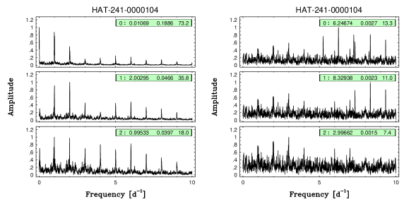
Figure 1: Panels on the left show the successive prewhitening of the raw test time series obtained by the injection of two sinusoidal components at 6.25 and 8.33 d^-1. Amplitudes are normalized, labels show the prewhitening cycle number, peak frequency, amplitude [mag] and signal-to-noise ratio. Simple Fourier prewhitening cannot recover the signal. Panels on the right show the result obtained by TFA filtering with $900$ templates. Both injected signal components are recovered with high significance.

One of the questions that can be asked is why direct Fourier filtering is not used to clean up the data from systematics. The reason is threefold: (i) there are systematics (e.g., transients) for which Fourier representation is a rather bad one; (ii) we do not know a priory which component can be treated as trend and which one as signal; (iii) for the most common periodic (daily) systematics Fourier filtering is less stable, because of the gaps in the data with the same periodicity. Figure 1 demonstrates the inadequacy of the simple Fourier filtering. The injected low-amplitude signal remains completely hidden if we employ direct Fourier filtering. Although TFA filtering also leaves some trend in the data (see the peak in the bottom right panel at $3.0$ d^-1), its amplitude is $26$-times smaller than that of the highest peak in the direct Fourier filtering at the same stage of prewhitening.

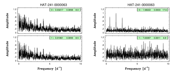
Figure 2: Example on a variable that is hidden in the raw time series (panels on the left) but becomes highly visible in the TFAd time series (panels on the right). Notation is as in Fig. 1.

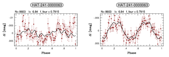
Figure 3: Folded/binned light curves with twice of the period of the variable shown in Fig. 2. Left: raw data, right: TFAd data. Headers from left to right: number of data points, average “I” magnitude, folding frequency in d^-1.

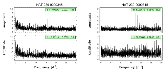
Figure 4: Example on a sub-millimag variable. The signal is detectable also in the raw time series (left) but is cleaner in the TFA filtered one (right). Notation is as in Fig. 2.

Next, in Fig. 2 we show the frequency spectra of a real variable that has escaped detection in the original time series. The star is rather bright and therefore it is strongly affected by various saturation-related effects. These effects are also common in other bright stars in the field, so it is possible to filter them out by employing TFA. In Fig. 3 we also show the folded light curves to give another look at the difference between the raw and the TFA-reconstructed results. Finally, as an example of the detection capability on the HATNet database, in Fig. 4 we show the frequency spectra of a sub-millimag variable.

Brief HATNet variability statistics

By using TFA post-processing, we have Fourier analyzed 10 HATNet fields in the $[0.0,20.0]$ d^-1 range and searched for variables with high significance (SNR$>10$) in the frequency spectra. The number of stars analyzed per field varies between 10000 and 25000, with 5000 to 11000 data points per object. The time spans covered by the observations are between 100 and 1000 days. The incidence rates of the variables are between 4 and 10%. The number of sub-mmag variables changes from field-to-field, but it is typically in the order of 100. All these statistics are, of course, strong functions of the data quality, time span of the observations and sample of objects. The total number of objects analyzed is 169000, covering a magnitude range of $7<V<13$. The number of variables is 9900. Some 12% of these are sub-mmag variables. For comparison, in an effort to produce a variable input catalog for the Kepler fields, Pigulski et al. (2008) analyzed 250000 objects from the ASAS database. They found a variability rate of 0.4%. This low incidence rate is not surprising if we consider that the average number of data points in these ASAS variables is only 100.